Abstract
Background
In heart data mining and machine learning, dimension reduction is needed to remove multicollinearity. Meanwhile, it has been proven to improve the interpretation of the parameter model. In addition, dimension reduction can also increase the time of computing in high dimensional data.
Methods
In this paper, we perform high dimensional ordination towards event counts in intensive care hospital for Emergency Department (ED 1), First Intensive Care Unit (ICU1), Second Intensive Care Unit (ICU2), Respiratory Care Intensive Care Unit (RICU), Surgical Intensive Care Unit (SICU), Subacute Respiratory Care Unit (RCC), Trauma and Neurosurgery Intensive Care Unit (TNCU), Neonatal Intensive Care Unit (NICU) which use the Generalized Linear Latent Variable Models (GLLVM’s).
Results
During the analysis, we measure the performance and calculate the time computing of GLLVM by employing variational approximation and Laplace approximation, and compare the different distributions, including Negative Binomial, Poisson, Gaussian, ZIP, and Tweedie, respectively. GLLVMs (Generalized Linear Latent Variable Models), an extended version of GLMs (Generalized Linear Models) with latent variables, have fast computing time. The major challenge in latent variable modelling is that the function is not trivial to solve since the marginal likelihood involves integration over the latent variable u.
Conclusions
In a nutshell, GLLVMs lead as the best performance reaching the variance of 98% comparing other methods. We get the best model negative binomial and Variational approximation, which provides the best accuracy by accuracy value of AIC, AICc, and BIC. In a nutshell, our best model is GLLVM-VA Negative Binomial with AIC 7144.07 and GLLVM-LA Negative Binomial with AIC 6955.922.
Supplementary Information
The online version contains supplementary material available at 10.1186/s12874-022-01538-4.
Keywords: GLLVM, Fast Computing, Laplace Approximation, Variational approximation, Ordination
Background
Big data is collecting massive data and is more complex, especially from new data sources [1]. The data set is large enough, so that software for traditional data processors is not good enough to manage it. Still, this massive amount of data can be used to overcome a variety of business problems that previously could not be solved for the decision-making [2]. The most straightforward and obvious explanation is that Big Data collects and uses various sources to provide important information. Big Data is also a concept of collecting, analysing, and understanding many data on a comprehensive range of activities. Big Data is profitable for the hospital service system. One of the classic problems is that there are excessively many staff or too few staff, so the hospital will risk incurring additional costs than they should. Not mainly that, hospitals that lose staff will also expose the quality and performance of the performed services.
If a few teams handle many patients, this will directly impact the services. These patients will be of poor quality and unsatisfactory. The primary key to implementing hospital orientation is the patient. Then, patient satisfaction is the success of a hospital in managing health care services. Customer satisfaction is an abstract thing, and the results are very varied.
However, perceptions depend on each person and tend to be different. The availability of medical personnel with high knowledge and skills is essential for patients choosing a health service to help them recover from the disease. The core business of the hospital is to provide health services. A good hospital can offer professional medical personnel and provide the best facilities and an excellent patient-care system [3]. At the same time, monitoring patient clinical status is essential, particularly in intensive care units (ICUs) [4]. During that time, the teleporter plays the role of “facilitator” and “supporter”. It is one of the medical team’s valuable members and the connection window between the unit and the department.
The transmission staff is responsible for assisting the patient’s medical treatment or acting as a helper for the family to care for the patient. It must have sufficient resilience to respond to the emergency that may occur, and the transmission process must strictly follow the actual transfer and relevant safety rules. The mastery, accuracy, and completeness of the delivery service time relate to the smooth connection of medical services, so it must have a certain degree of job sensitivity and excellent communication skills. Furthermore, with patients’ increasing needs and desires in obtaining the best services, it is necessary to do the proper planning, especially in the intensive care centre room.
The most crucial point is to place appropriate medical personnel in the intensive care centre. If the placement of medical staff is proper, hospital services will be better, and patients will be treated faster. Then another thing is to provide training to improve the work of medical personnel. If the human resources are of high quality and in line with company expectations, the company has high competitiveness. Therefore, the products and services produced high quality.
Intensive care units (ICUs) of university hospitals and advanced medical centres are indispensable for providing critical and intensive care for patients who have undergone major surgery or have received emergency care. Hospitals can obtain higher revenue from national insurance by a short admission in the ICU than by access to other hospital departments. Intensive care units are the foremost part and are very important in the hospital. Intensive care units act as the main entry gate for emergency patients and patients with mild conditions. Good or bad service in the intensive care unit will give an overall impression of hospital services. Analysing the number of events in the ICU is also essential to study. The cost estimation and a profit and loss analysis are necessary for the health care field [5].
A significant part of this work is to decide whether ICU care procedures can improve results for those identified as frailty. The instances of processes that may differ in the little incorporate wholesome help and sedation rehearse the force of assembly/restoration. In other words, an analysis of the number of medical personnel needs is essential in the ICU room; a first aid kit is needed quickly and temporarily to give a person suffering from an injury or sudden illness. First aid’s fundamental objective is to provide care and health services that benefit these people in preparation for further treatments.
An emergency is a condition related to a disease or other life-threatening illnesses. In contrast, a crisis is a sudden and unforeseen condition with an immediate or urgent need [6]. The emergency room’s operational nature must be fast, precise, and not limited by the time [7]. At the same time, we need to be concerned that the ideal performance of the emergency room is highly dependent on human resources and proper work procedures. Moreover, the supporting examination facilities can support the diagnostic process. The adequate drug support and medical consumables clear patients in and out, ready the operating room, and ambulance transport support that focuses on patient safety.
Big Data Analysis offers an excellent opportunity to improve strategic unit management and handle concrete clinical cases [8–10]. Moreover, different biomedical and medicinal services devices produce a primary information field measure [11]. We must think about and evaluate what can be accomplished by utilising this information field [12]. The problem is hard to select large-dimensional data; many attributes and causing some algorithms to be complex to get good performance. Therefore, the solution offered is to do feature selection or dimension reduction by using PCA [13–15], K-means [2], CCA [16], Factor analysis [17–19], eXtreme Gradient Boosting (XGBoost) [20–22] Bayesian [23–25].
Nowadays, there is challenging to measure statistical parameters in vast data sets, and most traditional statistical methods cannot handle high dimensional data and large numbers of parameters [24, 26–29]. This situation additionally typically mirrored the contemporary impediments of computing. In short, this research will get an ordinance of intensive care hospital rooms so that we can use it to calculate and predict how many patients are expected to be in the room daily and hourly. The remainder of the paper is organised as follows. Section 2 explains the methods. Section 3 presents the application of a high dimension. Section 4 presents the results and analysis. Finally, conclusions and future research directions are indicated in Sect. 4.
Methods
Generalized Linear Models
In its development, the modelling of count data led to Generalized Linear Models (GLMs) [8]. GLMs are generalisations of classical regression models or OLS regression. Analytical methods for data do not meet the assumption of a normal distribution [30]. The classical linear model is widely used in statistics or straight-line equation [31]. The traditional linear models were commonly used in statistics, especially for modelling field environmental problems [32]. The simplest classical non-linear model is defined in Eq. (1).
| 1 |
Where y is the dependent variable whose value depends on the independent variable x, β which are unknown parameters in the model. At the same time, ε is a random variable that differs from the actual value of y with its estimated value. The random variable ε is assumed to follow the Normal distribution . The development of the linear model was very rapid after discovering the normal distribution until the beginning of the 19th century that [33] published his research in agriculture using an experimental design. Simple GLMs are developing a classic linear model with many predictors or multiple linear regression [34]. The least-square method by Gauss remains the basis for estimating model parameters. The assumptions on LMs also carry over to GLMs is follows the Normal distribution . The predictor does not need continuous. Category predictors also underlie Fisher’s research in experimental design. Under the auspices of the normal distribution assumption, linear models can be written in general, or the general term defines GLM as in Eq. (2).
| 2 |
The model in Eq. (2) represents the GLMs for various linear models. They are linear regression (simple or multiple), multivariate regression, analysis of variance (ANOVA), multivariate analysis of variance (MANOVA), linear mixed models, analysis of variance-covariance (ANCOVA), multivariate analysis of covariance (MANCOVA), response surface, or growth curve model. In addition to the least square, parameter estimation can be obtained using the maximum likelihood, shrinkage estimation, stein-rule estimation method up to Bayes estimation approach. Operationalism means that scientific theories should be defined observably, namely observation or observational or experimental procedures.
In early 20th century, there have been many books published like “foundation of Statistics, the foundation of Ethics, foundation of justice, foundation of fairness” All of these books are studying foundational principles for their subjects, to enable deductive logic to justify necessary propositions of these areas [35–37]. Thus, in deductive logic if the general propositions are true, their logical statements also true, so that it would be called tautology, no error in their statements. However, how can we justify the truthfulness of claimed general propositions. The regression and generalized linear models (GLMs) describe the causal relationship between observed variables. is regarded as covariates, which cause the observed response to . Fisher’s classical likelihood applies to this kind of model with observables only, where fixed parameters represent causal effects of covariates. Via likelihood, the estimation of effects, prediction, various hypotheses testing, and including the absence of effects, have been developed [38–41].
Generalized Linear Latent Variable Models
Consider that are independent observations. Each represents response variable and each xi represents a vector of covariates, that is and to represent subjects. The joint distribution of can be written as the conditional distribution of given and the marginal distribution of We use the notation for the conditional distribution of given and for the marginal distribution of . The complete data density of ( for the subject i can be written as:
| 3 |
In the conditional distribution , is the vector of parameters. In our model, this parameter vector considers regression parameter through , zero inflation parameter or and over/under dispersion parameter , that is . In the marginal distribution, indicates the parameter of covariate distribution. We consider the natural exponential family distribution for the conditional distribution . For the following exponential family distribution, we consider parameter .
| 4 |
Where y represents the response variable, is the function of mean parameter , and is the function of scale parameter . The parameter is used to link the model to the covariates x. Let be a function of the linear predictor , that is , where f is a monotone differentiable function, known to be the link function and . In is the vector of covariates and is the vector of regression coefficients. If , then the link function f is said to be a canonical link function. We consider throughout our study, and hence would be written as or . The generalised linear model can be meaningless if many zeros in the information or over/under scattering highlight the information.
In the generalised linear model, covariates can be discrete, ceaseless, or both. We will portray the element in the next barely passages. This paper aims to develop GLLVMs with Laplace approximation and variational approximation based on the above analysis. The GLLVMs are the extended version of GLMs with latent variables. Suppose is the multivariate responses across species with being the observational units, and is the number of species. The expectation of is modelled through the following relationship.
| 5 |
The is the linear predictor and is a link function. The common link function is given in Table 1.
Table 1.
The Link function [42]
| Link Name | Link | Inverse | 1st Derivative |
|---|---|---|---|
| Gaussian/Normal | 1 | ||
| Binomial (Bernoulli: m=1) | |||
| Logit Probit | |||
| Log-log | |||
|
Poisson *Log |
|||
| Negatif Binomial *NB-C | |||
| Negatif Binomial *log | |||
|
Gamma *Inverse |
|||
|
Inverse Gaussian *Inv Quad |
The linear components of the predictor are similar to that of GLM has the inclusion of random effects listed as follows:
| 6 |
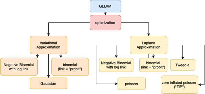
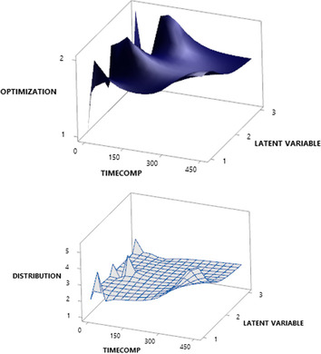
The represents the row effect, contains a matrix of the regression coefficient to corresponding independent variables. and are the loading factors or quantities describing the interactions across observation and connecting the unobserved variables to responses [43]. In many papers, the distributional choice of latent variables, is a normal distribution with mean zero and constant [44–46]. The optimisation in GLLVMs represents in Fig. 1.
Fig. 1.
GLLVMs Optimization
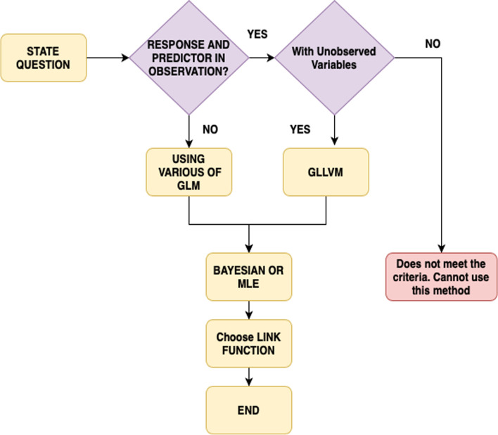
The selection of the distribution is another important point in GLM. The distribution preference is dependent on the type of response variable. The mechanism can produce the response and the form of the empirical distribution. For instance, the Bernoulli distribution is the obvious solution for binary responses, whereas the Poisson distribution is also preferred to match the model for counts. The intercept and the slope are also the key parameters to interpret in the standard multivariate regression. The interception is the outcome variable expectation unless the covariates remain zero. The regression coefficients reflect the anticipated variability in the dependent component variables for just a one-unit transition, with the remaining factor being consistent. The parameters may then be represented in Poisson and Negative Binomial methods as in Gaussian because of the log linking function that places variables in the normal log scale [47]. The result is exponential with the parameter through its main sample. This would not resolve the perception problem entirely, as represented in Fig. 2.
Fig. 2.
The concept for Choosing Latent GLMs and GLMs Family
Model Selection
The model selection criteria are statistical tools that identify an “optimal” statistical model from among a set of models. Meanwhile, the set is usually called a set of candidate models. A model is considered [48–50] that is the principle of generalizability to fit the model to describe or predict new data. The purpose of statistical modelling should be to predict new data instead of precisely characterising the actual model that generated the data. On the other hand, the candidate models are significant in analysing the selection criteria.
The criteria can be used Akaike Information Criterion (AIC), Akaike Information Criterion Correction (AICc), and Bayesian Information Criterion (BIC) [51]. Lastly, the selection of models should take generalizability, parsimony, and goodness-of-fit into account. The motivation behind measurable demonstrating ought to anticipate new information rather than unequivocally describe the genuine model that created the information. In Equation (7), f as the function of regression, k is the dimension of the parameter and n is the sample size.
| 7 |
| 8 |
| 9 |
However, the researcher leans toward BIC to AIC since BIC may prompt choosing a more closefisted fitted model than AIC. It demonstrates that BIC is steady, yet it is not asymptotically productive. In addition, AICc is helpful in the small dataset.
High dimension data
In this paper, we use the event count data that occur in the intensive care centre to meet the needs of medical operations. The operations include pushing hospitalised patients for hemodialysis treatment, receiving emergency treatment drugs, transferring specimens, and collecting blood and related services such as respirators, oxygen cylinders, and other equipment or items required for the treatment.
The data used in this research contains the number of events in the intensive care centre to meet the needs of medical operations in Taichung Veterans General Hospital. The specifications are as follows: Emergency Department (ED 1), First Intensive Care Unit (ICU1), Second Intensive Care Unit (ICU2), Respiratory Care Intensive Care Unit (RICU), Surgical Intensive Care Unit (SICU), Subacute Respiratory Care Unit (RCC), Trauma and Neurosurgery Intensive Care Unit (TNCU), Neonatal Intensive Care Unit (NICU). The data are collected from June (33,561 cases), July (31,557 cases), August (35,689 cases), September (34,293 cases), and October (35,310 cases). In total, the matrix dimension is (170,410 × 7). This paper only used eight types of ICU rooms. To get the ICU ordination per room will be transposed to (7 × 170,410). Then the dimension matrix is reduced again to retrieve the total daily occurrence data to get 153 × 7 a matrix. We estimate the latent space’s dimension from the data by using regularised generalised matrix factorisation [52].
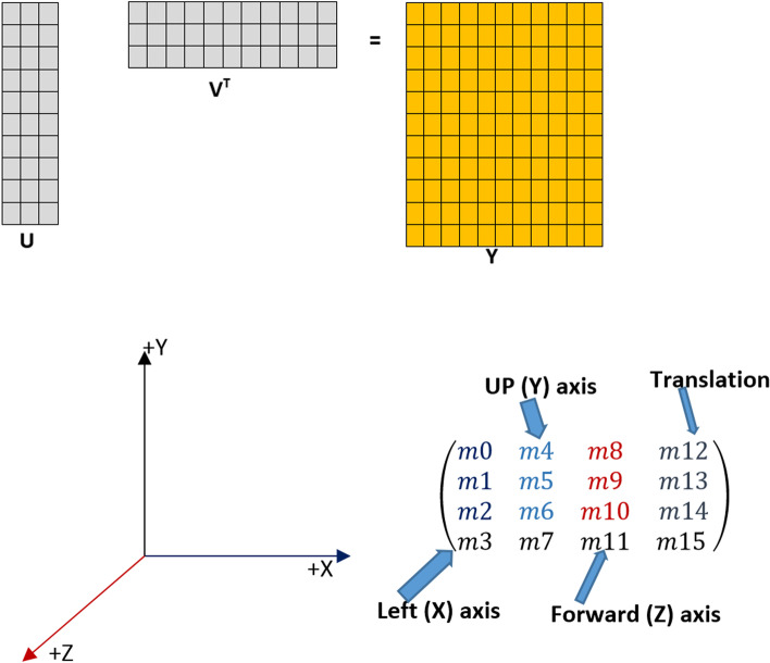
Since the dataset is a large size matrix with an observation sufficiently large, the approach would occur error. In the comparison, the method may be unreliable due to round-off errors for too short a break. We placed Newton Raphson (NR) in this analysis to solve these issues. The NR is not intermediate-based and approximates the Hessian matrix-vector product. The pseudo-Hessian matrices have been popularly used [53]. In this study, Fig. 3 represents that the pseudo-Hessian is applied because it has proven to be effective for , more instance see: [54].
Fig. 3.
The Example of Projection
Results and discussion
As explained in the previous section, we use the daily data of the number of cases of incentive care rooms. Then, the matrix dimension is quite large. So computation [55] will be calculated on selected distributions such as negative binomials, Poisson, Gaussian, ZIP, and Tweedie. We successfully compared two types of optimisation, including variational approximation and Laplace approximation. Also, we make a comparison with the number of latent variables. Table 2 explains that the best model is the smallest AIC, AICc, and BIC values for the negative distribution of GLLVM-VA and GLLVM-LA binomials. Figure 2a and b have explained that information. In general, VA (1) promises to complete computing time compared to LA (2).
Table 2.
GLLVMs Performance
| Model | LV | Family | Selection Criteria | DF | log-likelihood: | Time Computing | ||
|---|---|---|---|---|---|---|---|---|
| AIC | AICc | BIC | ||||||
| GLLVM- VA | 1 | Negative Binomial | 7144.07 | 7151.123 | 7207.709 | 21 | -3551.035 | 00.13,23 |
| 2 | Negative Binomial | 7309.096 | 7321.192 | 7390.918 | 27 | -3627.548 | 00.05,85 | |
| 3 | Negative Binomial | 7472.096 | 7489.696 | 7569.07 | 32 | -3704.048 | 00.06,11 | |
| 1 | Poisson | 7693.37 | 7699.733 | 7753.978 | 20 | -3826.685 | 00.01,22 | |
| 2 | Poisson | 7693.37 | 7699.733 | 7753.978 | 20 | -3826.685 | 00.03,60 | |
| 3 | Poisson | 7685.202 | 7695.439 | 7760.963 | 25 | -3817.601 | 00.12,20 | |
| 1 | Gaussian | 7260.324 | 7267.378 | 7323.964 | 21 | -3609.162 | 00.01,32 | |
| 2 | Gaussian | 7409.686 | 7421.782 | 7491.508 | 27 | -3677.843 | 00.03,42 | |
| 3 | Gaussian | 7570.224 | 7587.824 | 7667.198 | 32 | -3753.112 | 00.09,10 | |
| GLLVM- LA | 1 | Negative Binomial | 6955.922 | 6962.976 | 7019.562 | 21 | -3456.961 | 00.41,30 |
| 2 | Negative Binomial | -67622.6 | -67622.6 | -67622.6 | 27 | 3381132785 | 00.47,11 | |
| 1 | Poisson | 7736.851 | 7739.895 | 7779.277 | 14 | -3854.426 | 00.05,32 | |
| 2 | Poisson | 7387.098 | 7393.462 | 7447.707 | 20 | -3673.549 | 00.44,47 | |
| 3 | Poisson | 7227.31 | 7237.546 | 7303.07 | 25 | -3588.655 | 01.17,90 | |
| 1 | Gaussian | 7107.34 | 7114.393 | 7170.979 | 21 | -3532.67 | 00.01,72 | |
| 2 | Gaussian | 7103.672 | 7115.768 | 7185.494 | 27 | -3524.836 | 00.02,22 | |
| 3 | Gaussian | 7110.665 | 7128.265 | 7207.639 | 32 | -3523.333 | 00.01,88 | |
| 1 | ZIP | 7637.484 | 7644.538 | 7701.123 | 21 | -3797.742 | 00.31.38 | |
| 2 | ZIP | 7326.899 | 7338.995 | 7408.721 | 27 | -3636.449 | 00.59.18 | |
| 1 | Tweedie | 7010.549 | 7022.645 | 7092.371 | 27 | -3478.275 | 45.11,33 | |
Based on this simulation, we understand that the difference in latent variables does not affect the accuracy results. Besides, the recognisable proof of the estimation model is that it is sufficient for each latent variable. The decision of connection capacity ought to be founded on hypothetical contemplations and model fit. The scope of qualities it creates for the mean can be contemplated when picking the link function. For example, the logit and probit interface capacities are regular when the reaction variable is two-fold. They limit the likelihood within the interval . The other factors consider identifying with the understanding of the relapse parameters [55].
However, utilises an identity link function relates to addictive impacts of the covariates on the mean, and a log link compares to multiplicative effects. Another significant thing in GLLVMs is the decision of the dissemination. The decision of dissemination depends on the kind of reaction variable. The procedure produces the reaction and the state of experimental dispersion. For instance, the undeniable decision is the Bernoulli dissemination for parallel reactions while for counts. In line with this, the Poisson dispersion is regularly picked for fitting the model.
We use different distributions such as Negative Binomial (1), Poisson (2), Gaussian (3), ZIP (4), and Tweedie (5). As shown in Fig. 4, running a Tweedie distribution will take a very long time. The power parameters are vital to discuss. In tweedy probability density, it cannot be closed form so it is slow to finish computing. To solve this problem, quasi and pseudo-likelihood can be used for Tweedie.
Fig. 4.
Time Computing Optimization (A) and Type of Distribution (B)
The Tweedie distribution can only be analysed using the Laplace approximation GLLVM. Indeed, a Variational approximation is a Bayesian inference to solve complex statistics. Ormerod [56] gave a more precise explanation about the Variational approximation. On the other hand, Bayesian, along these lines [57] relies upon the researcher’s capacity to compute integrals concerning the posterior distribution. This is a troublesome issue and separated from the conjugate models. The explicit type of the thickness posterior is regularly accessible just to a factor.
During the experiment, we compare GLVVMs to PCA, Factor Analysis Extraction Maximum Likelihood, K-Means, Canonical Correlation Analysis, and Global Multidimensional Scaling. However, using K-means only uses two groups following the number of groups that have been previously determined. To determine the group members can be done by calculating the minimum distance of the object.
The value obtained in the membership of data at the distance matrix is 0 or 1. The value 1 is for data allocated to group A while the value 0 is for data allocated to group B. In this simulation, we obtained distance centroid (Cluster 1 to Cluster 2 = 24.6436). Table 3 provides variance information (%) of each method. During the experimental studies and the simulation results, GLLVMs promise high variance compared to the other techniques. In line with this, the number of variances can be explained with the latent variable as 98%. Yet, PCA and CCA perform variable reduction via justification and construct a scree plot variance explained (or eigenvalues).
Table 3.
The Variance
| Methods | Variance (%) |
|---|---|
| PCA | 78.5% |
| Factor Analysis Extraction Maximum Likelihood | 75.2% |
| K-Means 2 cluster | 51.070% |
| *Ours (GLLVM) | 98% |
| Canonical Correlation Analysis | 70.2% |
| Global Multidimensional Scaling | 68.5% |
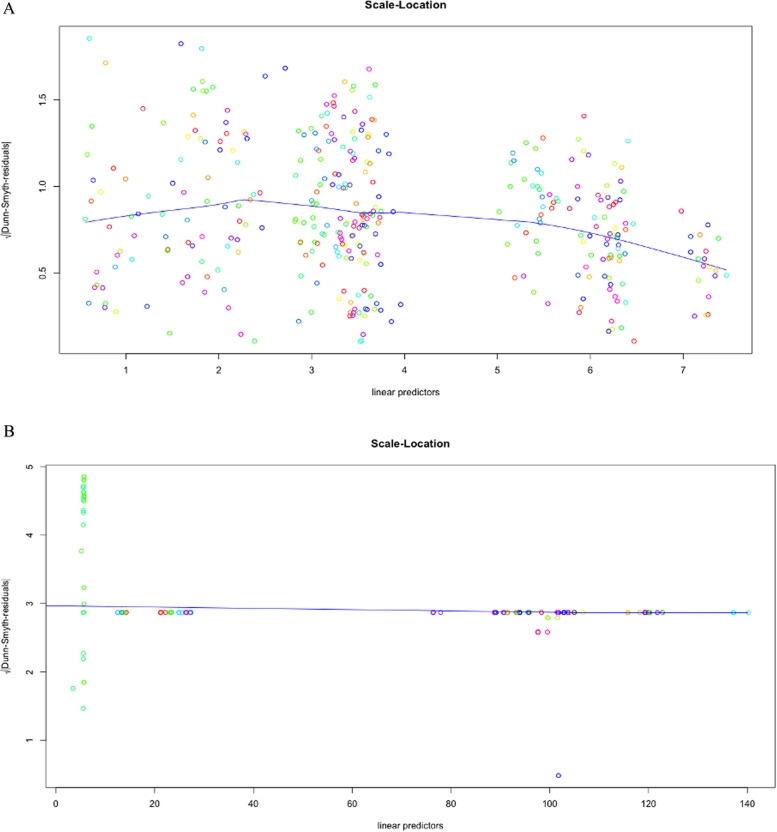
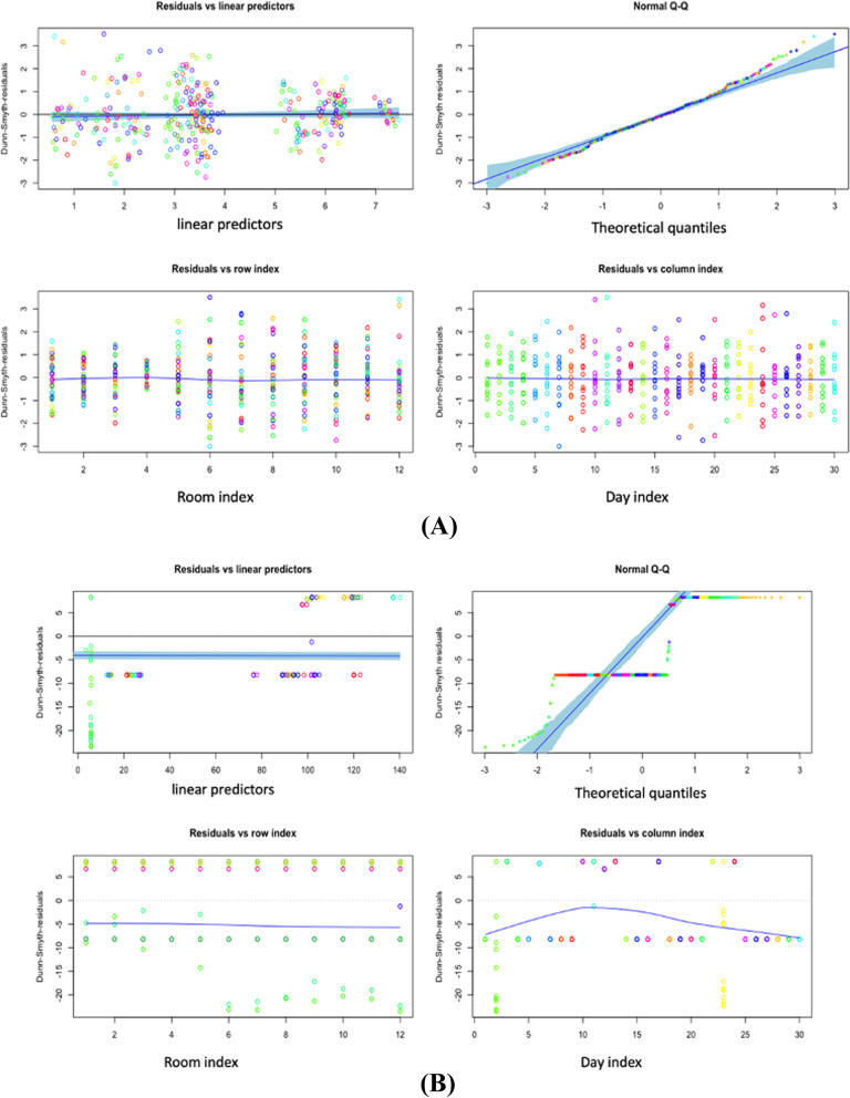
Meanwhile, two significant methodologies have shown up in measurements, such as approaches dependent on the characterisation of the posterior and approximation. For a differential condition, whose arrangement is not easy work at any rate. The Laplace approximation can tell the arrangement is the inverse Laplace likewise. The underlying conditions are folded into the strategy for the arrangement from the beginning. Nevertheless, with Bayes, we do not have the entirety of the underlying derivatives, so we need to keep some of them around as free parameters. The Laplace, for the most part, is not in nonlinear issues because we do not receive a decent arithmetical condition in return [, 58, 59]. One exception is that the Laplace change of a convolution is only an item helpful [60]. The data matrix is usually a proximity matrix (a matrix with a distance between objects) and includes ordinal data types. This result is robust because the configuration results are obtained from its iteration. However, the process will lose some information due to the reduction in dimensions. The ordination is also helpful in reducing the dimensions of data from several variables. New variables are no longer correlated and have as much information as possible from the original data after getting the best negative binomial model on two different optimisations, Variational approximation and Laplace approximation. It is necessary to find linear predictors with residuals in both models. Figure 5a and b represent scale location. At the beginning of our predictor range, the line starts off horizontal, slopes up to around 2, and then slopes down around 3. In the beginning, contrast with the Laplace approximation, the line is flattened around 2.5 because the residuals for those predictor values are not more spread out. The development of the GLLVM ordination will continue by using a Variational approximation. Assume that it provides speed in computing with accuracy differences that are not significant as the Laplace approximation. Figure 6a and b explain how linear these predictors are at residuals. Then, the normal Quantile-Quantile plot describes the theoretical quantiles following the normal distribution and the points forming a roughly straight line.
Fig. 5.
Scale Location GLLVM Negative Binomial with 1 Latent Variable Variational Approximation (A) Scale Location GLLVM Negative Binomial with 1 Latent Variable Laplace Approximation (B)
Fig. 6.
(A) GLLVM Negative Binomial with 1 Latent Variable Variational Approximation Residual VS Predictor (B) GLLVM Negative Binomial with 1 Latent Variable Laplace Approximation Residual VS Predictor
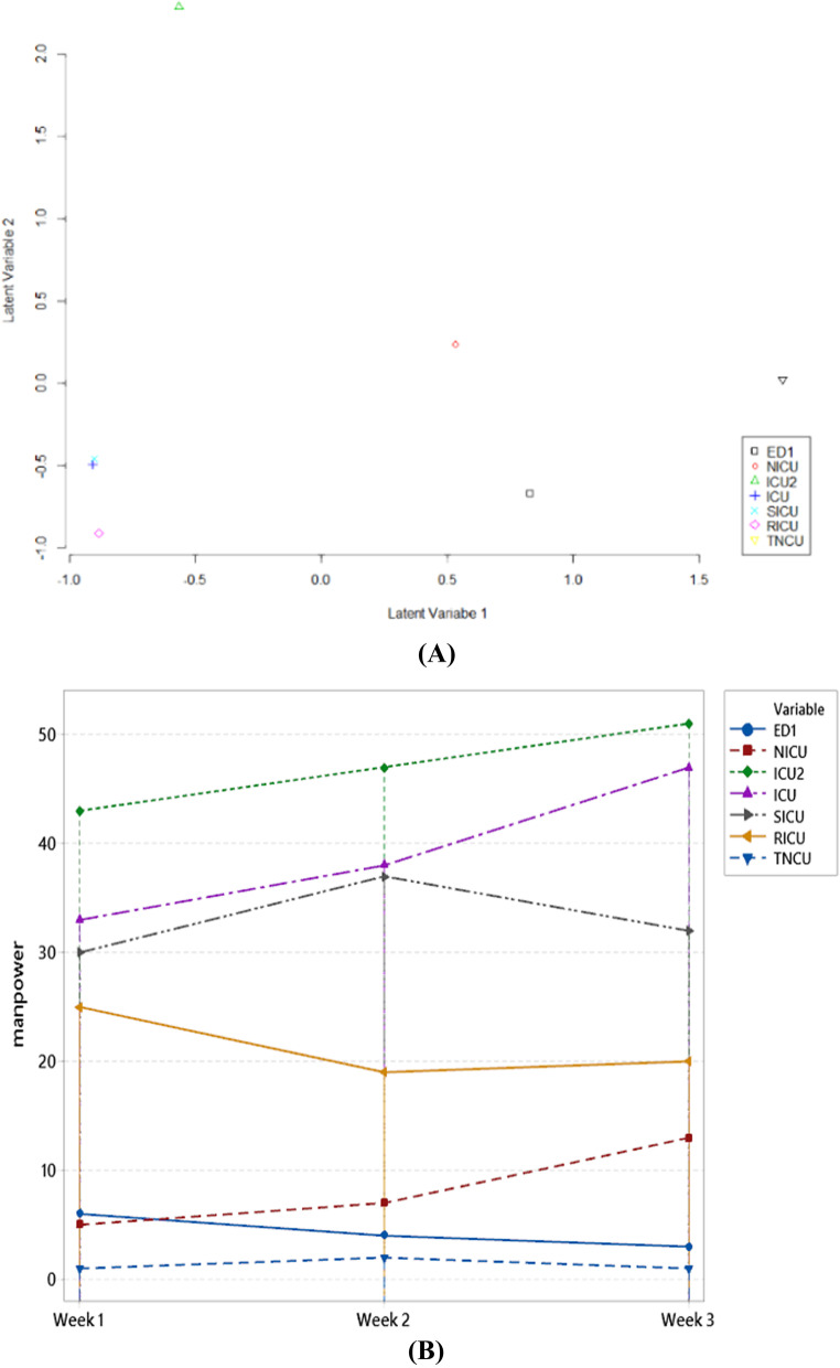
However, Fig. 7a explains the ordination in seven different room types. It seems so clear that each room has a different ordination. In addition, Fig. 7b represents the number of manpower based on the best model. The type of ICU room requires more manpower than other rooms. Nevertheless, visually ICU and RICU rooms have the same characteristics compared to the others. Overall, the different ordinance is ICU2 room, and separate ordinations are in the RICU room.
Fig. 7.
GLLVM Ordination (A) and Prediction manpower (B)
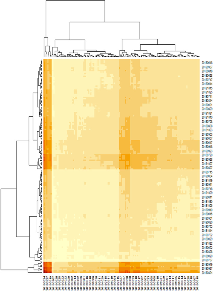
At the same time, the ordinations look similar in ED1 and TNCU rooms, respectively. Figure 8 explains the distribution of frequency of events data in intensive care Units’ rooms if there are several similarities between one day and another. The highest number of cases occurred on Monday and Saturday, and Sunday decreased quite far. If the hospital wants to focus on full service, it might be better to consider the appropriate number of medical staff on a specific day.
Fig. 8.
Heatmap event counts
The content of the hospital’s transfer staff is to transfer patients to outpatients, wards, inspections, and other units. The transfer methods include leadership, bed and wheelchair push, and the receipt and transfer of medicines, blood, specimens, articles, instruments, and stationery to other units. The outsourcing business of the hospital’s labour service is also to maintain the business activity. The staff is responsible for it, including the ward, medical department, or particular operation unit’s internal labour service. It is fixedly dispatched to the demand unit. Non-medical care services, such as ward replenishment, hand sanitiser, and redemption of infectious devices, medicine ladders, cleaning of dirty clothes, extra isolation clothes, etc., work items will follow the general ward. Moreover, the emergency characteristics of intensive or special controls and departmental treatment units may be different.
Still, their work is non-medical affairs, and responsible for such work belongs to internal staff. This mode’s transmission requirement is mainly related to the relevant operational processes required to treat inpatients. The examinations are X-rays, ultrasound, electrocardiograms, computed tomography (CT) tests or anesthesia visits before the operation of the patient; or pushing inpatients for blood Dialysis treatment, receiving emergency treatment medicines, transferring specimens, and related operations such as respirators, oxygen cylinders, and other equipment or items required for treatments.
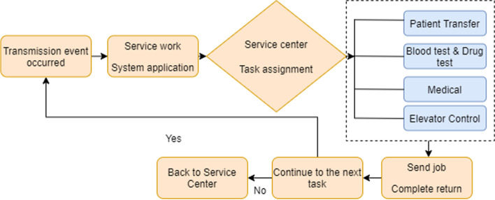
Figure 9 represents the application of the “Hospital Transfer Operating System” by the ward nursing station and the dispatching method which is based on the delivery center. The cases are general, urgent, or scheduled categories. The application event is transmitted to the service center to print the document. The service center dispatches personnel to perform the transmission operation and builds upon the priority of the event transmission or the application sequence. When the transmission staff completes the task, they return to the service center to wait for the next job assignment.
Fig. 9.
Hospital transfer operation flow
An ICU is an Intensive Care Unit, and CCU, for the most part, represents the Cardiac Care Unit. An emergency is a basic consideration unit that concedes therapeutic and careful patients who are fundamentally sick or harmed. While a Cardiac Care Unit concedes patients with heart issues, it is generally medicinal cardiovascular issues. The respiratory intermediate care unit (RICU) should be practically incorporated with the intensive care hospital room, the general ICU, and the restorative or different wards. These units should be described by higher self-sufficiency than the checking units because of the more elevated level of care [61].
Subsequently, while patients have the intense, the incessant respiratory disappointment of any level of seriousness ought to admit these units for the intubated individuals. Moreover, fundamentally sick patients with weaning issues could be admitted to the RICU. On the other hand, the Surgical Intensive Care Unit provides care for patients who have undergone many critical surgical procedures. SICU will cover Pediatric Vascular, Gastrointestinal Liver, Renal, Renal-Pancreas Transplantation, Orthopedics, Plastics, Otolaryngology, Urology, Thoracic, Surgical Oncology, Oral Maxillo-Facial Obstetrics, and Gynecological Surgery. Management of patient trauma is essential, and this treatment is carried out at the trauma care centre plus (TNCU).
Traumatic patients need airway evaluation and management, respiratory support, bleeding cases, rapid, swift. Patients who come to the emergency unit must go through triage, which evaluates the patient’s condition to determine the emergency level. Patients will be treated according to the category of triage, videlicet, triage one, patients with life-threatening conditions or loss of limb function and require immediate action or intervention with a waiting time of 0 min.
Then, triage two is a patient with a non-life-threatening condition but has a potential threat to limb function and requires prompt medical intervention or action with a waiting time of 0-5 min. Triage three are patients with acute conditions but not urgent (primarily stable). There is no potential to experience worsening and do not require immediate medical intervention or intervention with a waiting time of 5 to 15 min. NICU stands for neonatal intensive care unit, is an intensive care room in the hospital that is explicitly provided for newborns who experience health problems [62].
Generally, babies are placed into the NICU room in the first 24 h after birth. The length of stay in the NICU room varies, depending on each baby’s condition. The more serious the health problem is experienced, the longer they will be in the NICU room. There are many reasons why babies need to be cared for in the NICU room, but they aim to get the child under intensive supervision and care. The NICU room is a sterile area that just no one can enter. Each hospital has a different blueprint regarding the number and hours of parents visiting the NICU room. However, all hospitals must provide soap or hand sanitisers to ensure that visitors are sterile. In general, NICU room conditions are tranquil because they are susceptible to sound and light. The babies in the NICU room are usually in the incubator to keep their body temperature stable. The hospital delivery business is roughly divided into first, patient escort: during the patient’s medical treatment process. The patient is pushed for examination, surgery, kidney dialysis, or related treatment. Additionally, Non-patient is transmission: similar transmission of specimens, drugs, blood, documents, medical records, or medical supplies.
This research transmission business is aimed at front-open patient escort and non-patient transmission. According to the different work attributes of each ward, medical department, or operating unit, the required human resources are divided into four categories, and various types of human resources are ordered according to their complexity or danger.
Conclusions
This paper successfully performs the simulation of the huge dimensional dataset. The best distribution used is a negative binomial and variational approximation. Interestingly, the choice of the number of latent variables has a significant effect on computational time but not on the model’s accuracy. In general, the more latent used, it will slow down the computing time. The instrument involved the distribution of Tweedie was proven that Tweedie required a very long time compared to other distributions.
Future studies will use different types of distributions, such as extended negative binomials and hurdle distributions. We will compare the distribution zero-inflated Poisson, zero-inflated negative-binomial, beta-binomial, extended Poisson and Tweedie, hurdle, and extended hurdle for further research negative. In many situations, we cannot obtain information about which classes of some observations belong to which group. In this case, we need adaptations to the Variational Approximation and Laplace Approximation.
Posterior probabilities for labeled data do not need to be updated. The other probabilities corresponding to unlabeled data are computed as usual. Discussion, so far, assume that all the classes in the entire data sets are represented in the classes represented in labeled data so that GLLVM is known and model selection is not an issue. However, if the assumption does not hold, several problems arise with initialization on the optimization. One option is to consider only unlabeled information, ignoring the labeled observation. But, by considering and separating the dataset as training and testing, we can check our model is appropriate or not. In many multivariate data sets, some of the variables are highly correlated with others, so that they do not carry much additional information. The elimination of such variables can improve model performance. In Additional file 1: Appendix, We already explain how to calculate a computation of Variational Approximation and Laplace approximation. Otherwise, we may use the regularized log-likelihood function penalized by concern via where is the coordinate of the mean vector. Assume the independence of multinomial variables is the response to each spicy, with a p-response observed from each individual which can be modeled as a finite products-of-multinomials mixture model.
Future work should extend the basic concept of GLLVMs to Structural Equation Modelling (SEMs) or employ hierarchical likelihood. A frequentist alternative approach is proposed by Lee et al. [42], who termed it as the hierarchical likelihood approach. Hereafter, we use the term h-likelihood. Also, it provides a new way of statistical inferences in entire fields of statistical science. Recently, h-Likelihood is also commonly used for inferences and the application in big data and machine learning [63]. Therefore, we address the likelihood for fitting SEMs that supports various combinations of different distributions for response variables [48, 64–70]. h-likelihood can be defined by the logarithm of the joint density of the response and the unobserved vectors of random effects and given by
For estimation, we use for for for for and for [71].
Supplementary Information
Acknowledgements
The authors would like to thank the participants and staff of the Hospital Health Study for their valuable contributions.
Authors’ contributions
Conceptualization: REC,RCC Methodology: REC,RCC Project Administration: RCC,SWH,SYC,BP Software: REC Validation: REC Visualization: REC Writing – original draft, review and editing: REC,RCC Writing – original draft, review and editing: REC,RCC,SWH,SYC,PUG, and BP. The author(s) read and approved the final manuscript.
Funding
This work is part of the Ministry of Science and Technology, Taiwan, under Grant MOST 109-2622-E-324-004 and fully supported by Taichung Veterans General Hospital.
Availability of data and materials
The data that support the findings of this study are available from the corresponding author upon reasonable request.
Declarations
Ethics approval and consent to participate
Not applicable.
Consent for publication
Not applicable.
Competing interests
The authors declare that they have no competing interests.
Footnotes
Publisher’s Note
Springer Nature remains neutral with regard to jurisdictional claims in published maps and institutional affiliations.
Contributor Information
Rung-Ching Chen, Email: crching@cyut.edu.tw.
Su-Wen Huang, Email: dale33663366@vghtc.gov.tw.
References
- 1.Li Q, Lan L, Zeng N, You L, Yin J, Zhou X, et al. A Framework for Big Data Governance to Advance RHINs: A Case Study of China. IEEE Access. 2019;7.
- 2.Wang XD, Chen RC, Yan F, Zeng ZQ, Hong CQ. Fast Adaptive K-Means Subspace Clustering for High-Dimensional Data. IEEE Access. 2019;7:42639–51. doi: 10.1109/ACCESS.2019.2907043. [DOI] [Google Scholar]
- 3.Raheja JL, Dhiraj, Gopinath D, Chaudhary A. GUI system for elders/patients in intensive care. In: 2014 IEEE International Technology Management Conference, ITMC 2014. 2014.
- 4.Hever G, Cohen L, O’Connor MF, Matot I, Lerner B, Bitan Y. Machine learning applied to multi-sensor information to reduce false alarm rate in the ICU. J Clin Monit Comput. 2020;34:339–52. doi: 10.1007/s10877-019-00307-x. [DOI] [PubMed] [Google Scholar]
- 5.Cao P, Toyabe S ichi, Abe T, Akazawa K. Profit and loss analysis for an intensive care unit (ICU) in Japan: a tool for strategic management. BMC Health Serv Res. 2006;6:1. [DOI] [PMC free article] [PubMed]
- 6.Agresti A. An Introduction to Categorical Data Analysis. 2007. doi:10.1002/0471249688.
- 7.Capuzzo M, Moreno RP, Alvisi R. Admission and discharge of critically ill patients. Curr Opin Crit Care. 2010;16:499–504. doi: 10.1097/MCC.0b013e32833cb874. [DOI] [PubMed] [Google Scholar]
- 8.Ha I., Lee Y. Estimating Frailty Models via Poisson Hierarchical Generalized Linear Models. Journal of Computational and Graphical Statistics. 2003.
- 9.Ha I, Noh M, Lee Y, FrailtyHL A package for fitting frailty models with h-likelihood. R J. 2012;4:28–37. doi: 10.32614/RJ-2012-010. [DOI] [Google Scholar]
- 10.Dash S, Shakyawar SK, Sharma M, Kaushik S. Big data in healthcare: management, analysis and future prospects. J Big Data. 2019;6. doi:10.1186/s40537-019-0217-0.
- 11.Dimitrov DV. Medical internet of things and big data in healthcare. Healthc Inform Res. 2016;22:156–63. doi: 10.4258/hir.2016.22.3.156. [DOI] [PMC free article] [PubMed] [Google Scholar]
- 12.Viceconti M, Hunter P, Hose R. Big Data, Big Knowledge : Big Data for Personalized Healthcare. IEEE J Biomed Heal Informatics. 2015;19:1209–15. doi: 10.1109/JBHI.2015.2406883. [DOI] [PubMed] [Google Scholar]
- 13.Gower J, Lubbe S, Roux N le. Principal Component Analysis Biplots. In: Understanding Biplots. 2011.
- 14.Principal component analysis and redundancy analysis. In: Analysing Ecological Data. 2007.
- 15.Abdi H, Williams LJ. Principal component analysis. Wiley Interdisciplinary Reviews: Computational Statistics. 2010;2:433–59. doi: 10.1002/wics.101. [DOI] [Google Scholar]
- 16.ter Braak CJF, Verdonschot PFM. Canonical correspondence analysis and related multivariate methods in aquatic ecology. Aquat Sci. 1995.
- 17.Noh M, Lee Y, Oud JHL, Toharudin T. Hierarchical likelihood approach to non-Gaussian factor analysis. J Stat Comput Simul. 2019;89:1555–73. doi: 10.1080/00949655.2019.1590575. [DOI] [Google Scholar]
- 18.Jin S, Noh M, Lee Y. H-Likelihood Approach to Factor Analysis for Ordinal Data. Struct Equ Model. 2018;25:530–40. doi: 10.1080/10705511.2017.1403287. [DOI] [Google Scholar]
- 19.Bezdek JC, Ehrlich R, Full W. FCM: The fuzzy c-means clustering algorithm. Comput Geosci. 1984.
- 20.Mitchell R, Adinets A, Rao T, Frank E. XGBoost: Scalable GPU Accelerated Learning. 2018. http://arxiv.org/abs/1806.11248.
- 21.Chen RC, Caraka RE, Arnita, Goldameir NE, Pomalingo S, Rachman A, et al. An End to End of Scalable Tree Boosting System. Sylwan. 2020;165:1–11. [Google Scholar]
- 22.Nielsen D. Tree Boosting With XGBoost. 2016.
- 23.Caraka RE, Nugroho NT, Tai S-K, Chen RC, Toharudin T, Pardamean B. Feature Importance of The Aortic Anatomy on Endovascular Aneurysm Repair (EVAR) using Boruta and Bayesian MCMC. Commun Math Biol Neurosci. 2020;2020.
- 24.Johnstone IM, Titterington DM. Statistical challenges of high-dimensional data. Philosophical Transactions of the Royal Society A: Mathematical, Physical and Engineering Sciences. 2009. [DOI] [PMC free article] [PubMed]
- 25.Koch KR. Monte Carlo methods. GEM - Int J Geomathematics. 2018.
- 26.Choiruddin A, Coeurjolly JF, Letué F. Convex and non-convex regularization methods for spatial point processes intensity estimation. Electron J Stat. 2018;12:1210–55. doi: 10.1214/18-EJS1408. [DOI] [Google Scholar]
- 27.Choiruddin A, Cuevas-Pacheco F, Coeurjolly JF, Waagepetersen R. Regularized estimation for highly multivariate log Gaussian Cox processes. Stat Comput. 2019;:1–14.
- 28.Niku J, Hui FKC, Taskinen S, Warton DI. gllvm: Fast analysis of multivariate abundance data with generalized linear latent variable models in r. Methods Ecol Evol. 2019;:1–10.
- 29.Hao L, Kim J, Kwon S, Ha I, Do Deep learning-based survival analysis for high-dimensional survival data. Mathematics. 2021;9:1–18. [Google Scholar]
- 30.Cox DD, John S. A statistical method for global optimization. In: Conference Proceedings - IEEE International Conference on Systems, Man and Cybernetics. 1992. p. 1–15.
- 31.Bates DM, Watts DG. Review of Linear Regression. Nonlinear Regres Anal Its Appl. 1988;:1–31. doi:10.1002/9780470316757.ch1.
- 32.Militino AF. Mixed Effects Models and Extensions in Ecology with R. J R Stat Soc Ser A (Statistics Soc. 2010.
- 33.Lury DA, Fisher RA. Statistical Methods for Research Workers. Stat. 1972.
- 34.Goldstein H, Cohen J, Cohen P. Applied Multiple Regression/Correlation Analysis for the Behavioural Sciences. J R Stat Soc Ser A. 1976.
- 35.Freedman D. Some issues in the foundation of statistics. Dordrecht: Springer; 1997. [Google Scholar]
- 36.Savage LJ. The foundations of statistics. Courier; 1972.
- 37.Čencov NN. Algebraic foundation of mathematical statistics. Ser Stat. 1978;9:267–76. doi: 10.1080/02331887808801428. [DOI] [Google Scholar]
- 38.Hall DB. Zero-inflated poisson and binomial regression with random effects: A case study. Biometrics. 2000. [DOI] [PubMed]
- 39.Ha ID, Lee Y. Multilevel mixed linear models for survival data. Lifetime Data Anal. 2005;11:131–42. doi: 10.1007/s10985-004-5644-2. [DOI] [PubMed] [Google Scholar]
- 40.Ha I., Jeong J-H, Lee Y. Statistical Modelling of Survival Data with Random Effects H-Likelihood Approach. Springer; 2017.
- 41.Lee Y, Nelder JA. Hierarchical Generalized Linear Models. J R Stat Soc Ser B. 1996. [DOI] [PubMed]
- 42.Lee Y, Rönnegård L, Noh M. Data analysis using hierarchical generalized linear models with R. 1st edition. Florida: Routledge; 2017.
- 43.Caraka RE, Chen RC, Lee Y, Toharudin T, Rahmadi C, Tahmid M, et al. Using multivariate generalized linear latent variable models to measure the difference in event count for stranded marine animals. Glob J Environ Sci Manag. 2021;7:117–30. [Google Scholar]
- 44.Warton DI. Many zeros does not mean zero inflation: Comparing the goodness-of-fit of parametric models to multivariate abundance data. Environmetrics. 2005;16:275–89. doi: 10.1002/env.702. [DOI] [Google Scholar]
- 45.Warton DI, Foster SD, De’ath G, Stoklosa J, Dunstan PK. Model-based thinking for community ecology. Plant Ecol. 2015.
- 46.Niku J, Brooks W, Herliansyah R, Hui FKC, Taskinen S, Warton DI. Efficient estimation of generalized linear latent variable models. PLoS One. 2019;14:1–20. doi: 10.1371/journal.pone.0216129. [DOI] [PMC free article] [PubMed] [Google Scholar]
- 47.del Castillo J, Lee Y. GLM-methods for volatility models. Stat Modelling. 2008;8:263–83. doi: 10.1177/1471082X0800800303. [DOI] [Google Scholar]
- 48.Jin S, Ankargren S. Frequentist Model Averaging in Structural Equation Modelling. Psychometrika. 2019;84:84–104. doi: 10.1007/s11336-018-9624-y. [DOI] [PubMed] [Google Scholar]
- 49.Bartholomew D, Knott M, Moustaki I. Latent Variable Models and Factor Analysis: A Unified Approach: 3rd Edition. 2011.
- 50.Myers RH, Montgomery DC, Vining GG, Robinson TJ. Generalized Linear Models: With Applications in Engineering and the Sciences: Second Edition. 2012.
- 51.Lee D, Kang H, Kim E, Lee H, Kim H, Kim YK, et al. Optimal likelihood-ratio multiple testing with application to Alzheimer’s disease and questionable dementia Data analysis, statistics and modelling. BMC Med Res Methodol. 2015;15:1–11. doi: 10.1186/1471-2288-15-9. [DOI] [PMC free article] [PubMed] [Google Scholar]
- 52.Kidziński L, Hui FKC, Warton DI, Hastie T. Generalized Matrix Factorization. arXiv Prepr. 2020. http://arxiv.org/abs/2010.02469. [PMC free article] [PubMed]
- 53.Sum J, Leung CS, Young GH, Kan WK. On the Kalman filtering method in neural-network training and pruning. IEEE Trans Neural Networks. 1999;10:161–6. doi: 10.1109/72.737502. [DOI] [PubMed] [Google Scholar]
- 54.Lue HH. On principal Hessian directions for multivariate response regressions. Comput Stat. 2010;25:619–32. doi: 10.1007/s00180-010-0192-6. [DOI] [Google Scholar]
- 55.Herliansyah R, Fitria I. Latent variable models for multi-species counts modeling in ecology. Biodiversitas. 2018.
- 56.Ormerod JT, Wand MP. Explaining variational approximations. Am Stat. 2010;64:140–53. doi: 10.1198/tast.2010.09058. [DOI] [Google Scholar]
- 57.Tzikas DG, Likas AC, Galatsanos NP. The variational approximation for Bayesian inference. IEEE Signal Process Mag. 2009.
- 58.Shun Z, McCullagh P. Laplace Approximation of High Dimensional Integrals. J R Stat Soc Ser B. 1995.
- 59.Adibi A. Semiconductor Device Simulation by a New Method of Solving Poisson, Laplace and Schrodinger Equations. Int J Eng. 2000;13:89–94. [Google Scholar]
- 60.Mohammadpoory Z, Haddadnia J. Speech Enhancement Using Laplacian Mixture Model under Signal Presence Uncertainty. Int J Eng. 2014;27(9):1367–76. [Google Scholar]
- 61.Corrado A, Roussos C, Ambrosino N, Confalonieri M, Cuvelier A, Elliott M, et al. Respiratory intermediate care units: A European survey. Eur Respir J. 2002;20:1343–50. doi: 10.1183/09031936.02.00302602. [DOI] [PubMed] [Google Scholar]
- 62.Losiouk E, Lanzola G, Galderisi A, Trevisanuto D, Steil GM, Facchinetti A, et al. A telemonitoring service supporting preterm newborns care in a neonatal intensive care unit. In: RTSI 2017 - IEEE 3rd International Forum on Research and Technologies for Society and Industry, Conference Proceedings. 2017.
- 63.Caraka RE, Noh M, Chen RC, Lee Y, Gio PU, Pardamean B. Connecting Climate and Communicable Disease to Penta Helix Using Hierarchical Likelihood Structural Equation Modelling. Symmetry (Basel) 2021;13:1–21. [Google Scholar]
- 64.Jin S. Essays on Estimation Methods for Factor Models and Structural Equation Models. Uppsala: Acta Universitatis Upsaliensis; 2015. [Google Scholar]
- 65.Jin S, Lee Y. A review of h-likelihood and hierarchical generalized linear model. WIREs Comput Stat. 2020;July:1–23. doi: 10.1002/wics.1527. [DOI] [Google Scholar]
- 66.Jin S, Vegelius J, Yang-Wallentin F. A Marginal Maximum Likelihood Approach for Extended Quadratic Structural Equation Modeling with Ordinal Data. Struct Equ Model. 2020;27:864–73. doi: 10.1080/10705511.2020.1712552. [DOI] [Google Scholar]
- 67.Jin S, Noh M, Yang-Wallentin F, Lee Y. Robust nonlinear structural equation modeling with interaction between exogenous and endogenous latent variables. Struct Equ Model. 2021;:1–10.
- 68.Felleki M, Lee D, Lee Y, Gilmour AR, Rönnegård L. Estimation of breeding values for mean and dispersion, their variance and correlation using double hierarchical generalized linear models. Genet Res (Camb) 2012;94:307–17. doi: 10.1017/S0016672312000766. [DOI] [PubMed] [Google Scholar]
- 69.Lee Y, Noh M. Modelling random effect variance with double hierarchical generalized linear models. Stat Modelling. 2012;12:487–502. doi: 10.1177/1471082X12460132. [DOI] [Google Scholar]
- 70.Lee Y, Rönnegård L, Noh M, Lee Y, Rönnegård L, Noh M. Double HGLMs - Using the dhglm Package. In: Data Analysis Using Hierarchical Generalized Linear Models With R. 2017.
- 71.Caraka RE, Lee Y, Chen RC, Toharudin T. Using Hierarchical Likelihood towards Support Vector Machine: Theory and Its Application. IEEE Access. 2020;8:194795–807. doi: 10.1109/ACCESS.2020.3033796. [DOI] [Google Scholar]
Associated Data
This section collects any data citations, data availability statements, or supplementary materials included in this article.
Supplementary Materials
Data Availability Statement
The data that support the findings of this study are available from the corresponding author upon reasonable request.


