Abstract
Deep eutectic solvents (DES) are recently synthesized to cover limitations of conventional solvents. These green solvents have wide ranges of potential usages in real-life applications. Precise measuring or accurate estimating thermophysical properties of DESs is a prerequisite for their successful applications. Density is likely the most crucial affecting characteristic on the solvation ability of DESs. This study utilizes seven machine learning techniques to estimate the density of 149 deep eutectic solvents. The density is anticipated as a function of temperature, critical pressure and temperature, and acentric factor. The LSSVR (least-squares support vector regression) presents the highest accuracy among 1530 constructed intelligent estimators. The LSSVR predicts 1239 densities with the mean absolute percentage error (MAPE) of 0.26% and R2 = 0.99798. Comparing the LSSVR and four empirical correlations revealed that the earlier possesses the highest accuracy level. The prediction accuracy of the LSSVR (i.e., MAPE = 0. 26%) is 74.5% better than the best-obtained results by the empirical correlations (i.e., MAPE = 1.02%).
Subject terms: Chemical engineering, Materials chemistry
Introduction
The separation-based equipment has always been an accompanied part of chemical processes1, pharmaceutical industries2, water/wastewater treatment processes3–5, and environmental protection6. The separation process primary responsibility is to remove contaminants from feed stocks and effluent liquid and gas streams, purify final products, and recover unreacted materials7. Although diverse separation processes have already been established, the solvent-based technique has a wider range of applications.
The green chemistry principles introduced by Anastas and Warner suggested constructing chemical processes that eliminate or at least reduce utilizing/generating harmful substances8. Since the traditional organic solvents undesirably impact the ecosystem and human health, researchers have paid great attention to synthesizing green, sustainable, and environmentally-friendly solvents. Attempts to fulfill this objective have resulted in suggesting supercritical fluids9, renewable solvents10, liquid polymers11, and ionic liquids12.
Deep eutectic solvents (DES) have recently been recommended as materials that have the favorable features of ionic liquids and cover their undesirable characteristics13–16. Deep eutectic solvents have readily been synthesized by mixing two main agents, i.e., hydrogen bond donor (HBD) and hydrogen bond acceptor (HBA)17. Hydrogen bond formations between HBA and HBD resulted in synthesizing a mixture with a melting point highly smaller than its ingredient17. Generally, deep eutectic solvents are biodegradable, inexpensive, non-toxic, non-volatile, thermally/chemically stable, and easy to manufacture17.
Despite a short life of deep eutectic solvents, they have engaged in diverse applications, including material synthesis18, separation processes13, nanotechnology19, environmental protection17, biotechnology20, and pharmaceutical processing21.
The accurate values of volumetric properties of deep eutectic solvents, like density, are essential for feasibility study and detailed design of any possible industrial usages of DESs22. Moreover, selecting an appropriate DES with the desired density is an arduous task to be accomplished through laboratory-scale investigations.
Therefore, constructing a predictive tool to anticipate the density of deep eutectic solvents may be helpful in this regard. Although a few empirical correlations have technically been built for estimating the density of DESs (see Sect. 3.1), to the best of our knowledge, no intelligent scheme has been suggested yet. Hence, this work utilizes five intelligent schemes for calculating the DES’s density from some available variables, i.e., temperature and DES’s inherent features (acentric factor and critical pressure and temperature) and compares their prediction accuracy. This is the most comprehensive modeling study yet conducted for mechanizing the DES’s characterization. The databank includes massive laboratory-scale density measurements gathered from the literature to certify that the suggested paradigms are general and robust. The reliability of the constructed intelligent estimators is higher than the other correlations proposed in the literature.
Laboratory-measured datasets
The objective of the current study is constructing an intelligent tool to approximate the density of deep eutectic solvents precisely. Identical to the regression-based correlation23, all intelligent methods also need a laboratory-measured database to adjust their parameters and test their prediction reliability24,25. Thus, 1239 experimentally measured datasets for the density of deep eutectic solvents have been gathered from thirty references and engaged in the model development/validation stage. The summary of the collected density data has been presented in Table 1. This table introduces the name of hydrogen bond donors and hydrogen bond acceptors of the considered deep eutectic solvents. As Table 1 shows, the gathered databank includes thirteen HBA and forty-two HBD ingredients. This table also indicates the number of measurements and ranges of the working temperature and measured density.
Table 1.
Summary of the reported laboratory-measured density for diverse deep eutectic solvents in the literature.
| HBA agent | HBD agent | Temperature range (K) | Density range (kg/m3) | Numbers of data | References |
|---|---|---|---|---|---|
| Acetyl choline chloride (HBA #1) | 1,2,4-triazole, D-Fructose, D-Glucose, D-Mannose, D-Ribose, D-Xylose, Guaiacol, Imidazole, Levulinic acid | 293.15–363.15 | 1089.5–1275.0 | 120 | 13–16 |
| Allyl triphenylphosphonium bromide (HBA #2) | Diethylene glycol, Triethylene glycol | 293.15–343.15 | 1108.4–1201.1 | 66 | 17 |
| Benzyl tripropyl ammonium Chloride (HBA #3) | Ethylene glycol, Glycol, Lactic acid, Oxalic acid, Phenol | 293.15–348.15 | 1027.6–1263.0 | 56 | 30 |
| Betaine (HBA #4) | Lactic acid, Levulinic acid | 293.15–343.15 | 1126.6–1208.9 | 32 | 31 |
| Benzyldimethyl (2-hydroxyethyl) ammonium chloride (HBA #5) | D-Fructose, D-Glucose, D-Mannose, D-Ribose, D-Xylose | 293.15–353.15 | 1192.0–1262.0 | 65 | 14 |
| Choline chloride (HBA #6) | 1,2-propanediol, 1,4-butanediol, 2,3-butanediol, Acetamide, Citric acid, D-Fructose, D-Glucose, D-Mannose, D-Ribose, D-Sorbitol, D-Sucrose, D-Xylose, Ethylene glycol, Glycolic, Glycolic acid, Guaiacol, Levulinic acid, Malonic acid, N-furfuryl alcohol, O-Cresol, Oxalic acid, P-Chlorophenol, P-Cresol, Phenol, p-Toluenesulfonic acid, Tartaric acid, Triethylene glycol, Urea, Xylitol | 283.15–368.15 | 1019.7–1350.0 | 439 | 14–16,19,32–48 |
| Diethylamine hydrochloride (HBA #7) | Guaiacol | 293.15–323.15 | 1075.8–1106.1 | 12 | 15 |
| L-proline (HBA #8) | Lactic acid, Levulinic acid | 293.15–343.15 | 1164.0–1265.1 | 22 | 31 |
| Methyl triphenylphosphonium bromide (HBA #9) | Ethylene glycol, Glycerol | 298.15–368.15 | 1168.8–1306.4 | 105 | 47,49 |
| N, N diethylenethanol ammonium chloride (HBA #10) | Ethylene glycol, Glycerol | 298.15–368.15 | 1054.6–1220.1 | 110 | 33,47 |
| Tetrabutylammonium chloride (HBA #11) | Arginine, Aspartic acid, Ethylene glycol, Glutamic acid, Glycerol, Phenylacetic acid, Propionic acid, Triethylene glycol, Levulinic acid | 288.15–353.15 | 928.0–1154.0 | 158 | 16,17,50,51 |
| Tetraethylammonium bromide (HBA #12) | Levulinic acid, Ethylene glycol, Glycerol | 293.15–343.15 | 975.7–1177.4 | 33 | 16,52 |
| Trimethylglicine (HBA #13) | 2-Chloro benzoic acid, Benzoic acid, Mandelic acid, Phenylacetic acid | 298.15–373.15 | 1110.0–1290.0 | 21 | 53 |
Critical pressure, critical temperature, and acentric factor
This study aims to build a single model to anticipate the density of 149 various deep eutectic solvents. Therefore, it is mandatory to include inherent characteristics of these materials in the list of independent variables. The three-parameter corresponding state theory explains that each material has its own specific acentric factor, critical temperature, and critical pressure26. Hence, these parameters could help the machine learning method distinguish different deep eutectic solvents and discriminate among their density values27. Haghbakhsh et al.28 utilized the improved Lydersen-Joback–Reid group contribution12 and the Lee-Kesler mixing rules29 to estimate acentric factor and critical temperature/pressure of different deep eutectic solvents.
Table 2 presents the range of these inherent characteristics for all considered deep eutectic solvents28. The supplementary excel files includes all experimental databank utilized in the current study.
Table 2.
The reported critical pressure, critical temperature, and acentric factor for the considered deep eutectic solvents28.
| HBA agent | HBD agent | Range of Tc (K) | Range of Pc (MPa) | Range of ω (-) |
|---|---|---|---|---|
| Acetylcholine chloride | 1,2,4-triazole, D-Fructose, D-Glucose, D-Mannose, D-Ribose, D-Xylose, Guaiacol, Imidazole, Levulinic acid | 635.41–846.26 | 2.3489–4.7708 | 0.4154–1.4097 |
| Allyl triphenylphosphonium bromide | Diethylene glycol, Triethylene glycol | 696.23–817.24 | 2.5162–3.4033 | 0.9700–1.0819 |
| Benzyl tripropyl ammonium chloride | Ethylene glycol, Glycol, Lactic acid, Oxalic acid, Phenol | 644.10–744.01 | 2.7293–3.7822 | 0.5152–1.2862 |
| Betaine | Lactic acid, Levulinic acid | 668.50–701.24 | 3.8938–4.7230 | 0.6195–0.8755 |
| Benzyldimethyl (2-hydroxyethyl) ammonium chloride | D-Fructose, D-Glucose, D-Mannose, D-Ribose, D-Xylose | 843.35–908.27 | 2.1009–2.4724 | 1.3871–1.5684 |
| Choline chloride | 1,2-propanediol, 1,4-butanediol, 2,3-butanediol, Acetamide, Citric acid, D-Fructose, D-Glucose, D-Mannose, D-Ribose, D-Sorbitol, D-Sucrose, D-Xylose, Ethylene glycol, Glycolic, Glycolic acid, Guaiacol, Levulinic acid, Malonic acid, N-furfuryl alcohol, O-Cresol, Oxalic acid, P-Chlorophenol, P-Cresol, Phenol, p-Toluenesulfonic acid, Tartaric acid, Triethylene glycol, Urea, Xylitol | 600.98–1084.19 | 2.4301–5.2851 | 0.4770–1.5011 |
| Diethylamine hydrochloride | Guaiacol | 680.55–694.99 | 4.3476–4.5308 | 0.4659–0.4737 |
| L-proline | Lactic acid, Levulinic acid | 721.95–745.61 | 4.2880–4.8538 | 0.7044–0.8243 |
| Methyl triphenylphosphonium bromide | Ethylene glycol, Glycerol | 666.50–843.78 | 2.8329–4.2132 | 0.9031–1.2929 |
| N, N diethylenethanol ammonium chloride | Ethylene glycol, Glycerol | 604.66–699.38 | 3.2396–4.4874 | 0.9195–1.3207 |
| Tetrabutylammonium chloride | Arginine, Aspartic acid, Ethylene glycol, Glutamic acid, Glycerol, Phenylacetic acid, Propionic acid, Triethylene glycol, Levulinic acid | 588.75–808.05 | 1.4380–4.1852 | 0.6212–1.3576 |
| Tetraethylammonium bromide | Levulinic acid, Ethylene glycol, Glycerol | 687.77–793.24 | 1.9639–2.8859 | 0.6275–1.3155 |
| Trimethylglycine | 2-Chloro benzoic acid, Benzoic acid, Mandelic acid, Phenylacetic acid | 711.92–780.73 | 3.5488–4.0881 | 0.5609–0.8301 |
In order to reduce the table size, the reported values have been presented for deep eutectic solvents based on their hydrogen bond acceptor type. Specific values of the acentric factor, critical temperature, and critical pressure for each deep eutectic solvent can be found in Haghbakhsh et al. article28.
Estimation scenarios for density of deep eutectic solvents
The literature has suggested several empirical correlations for estimating the liquid’s density. Furthermore, the current study focuses on seven machine learning methods to anticipate the density of 149 deep eutectic solvents. The mathematical formulation/background of the available empirical correlations and machine learning methods has been briefly reviewed in this section.
Empirical correlations
Rackett correlation
Rackett’s correlation is likely the first equation developed to calculate the saturated liquid’s density54. As Eq. (1) explains, the molar volume () is estimated as a function of temperature (T) and critical pressure (Pc), molar volume (), and temperature (Tc). R and Tr show the gas constant and reduced temperature (Eq. 2), respectively.
| 1 |
| 2 |
Equation (3) is then possible to be used to reach the density () from the molecular weight (M) and estimated molar volume.
| 3 |
Although Rackett’s correlation was initially suggested for the saturated liquid’s density, it has also presented good predictions for the deep eutectic solvent55.
Spencer and Danner correlation
Spencer and Danner incorporate a base molar volume measurement () at a base temperature () in Rackett’s correlation56. Equations (4) and (5) introduce the modified Rackett model, i.e., the Spencer and Danner correlation.
| 4 |
| 5 |
Mjalli et al. correlation
Mjalli et al.57 suggested a technical correlation for the density of deep eutectic solvents by reformulating the Spencer and Danner model. Equations (6) and (7) express the mathematical shape of the developed correlation by Mjalli et al.57.
| 6 |
| 7 |
Haghbakhsh et al. correlation
Haghbakhsh et al. recently proposed a correlation for calculating the density of deep eutectic solvents from the working and critical temperatures, acentric factor (ω), and critical molar volume28.
| 8 |
| 9 |
It can be seen that all empirical correlations utilize the temperature and inherent characteristics of the material (a combination of the νc, Pc, Tc, and ω) to formulize the liquid’s density. Since the first three inherent properties (Tc, Pc, and νc) are related through the following equation, it is unnecessary to utilize all of them.
| 10 |
Therefore, the current study only utilizes temperature, Tc, Pc, and ω to estimate the DES’s density employing different intelligent estimators (Eq. 11).
| 11 |
Computational intelligent methods
Wide ranges of supervised and unsupervised artificial intelligence techniques have been suggested and applied in different modeling studies58–63. The working procedures of the used machine learning methods, i.e., least-squares support vector regression (LSSVR), hybrid neuro-fuzzy system, and five types of artificial neural networks have been briefly explained in this section.
Least-squares support vector regression
This intelligent estimator employs a particular equation (i.e., linear, Gaussian, and polynomial kernel function) to transfer original independent variables () to a multi-dimensional computational domain. The following equation defines these functions.
| 12 |
The superscript of T shows the transpose operation. In addition, , , and are the kernel-related parameters.
It is then possible to linearly relate the dependent () to the independent () variables in this new computational domain utilizing Eq. (13).
| 13 |
In Eq. (13), represents the estimated target by the least-squares support vector regression. Furthermore, w and b are adjustable coefficients of this intelligent model. In summary, the kernel type is the main topology feature of the LSSVR that should be determined by a practical scenario like the trial-and-error process64.
The detailed working process of the least-squares support vector machine has recently been explained by Nabavi et al.64.
Artificial neural networks
This neuron-based machine learning method is the most widely-used tool as either estimator65,66 or classifier67. The working process of the artificial neural network is handled by a combination of linear (LPart) and non-linear (NLPart) operations conducted by the neuron as follows68:
| 14 |
| 15 |
w, b, and are weight and bias coefficients and activation function, respectively. Although a linear activation function exists, the non-linear, continuous, and differentiable ones often provide artificial neural networks with a better generalization ability69. Equation (16) defines several widely-used activation functions in the field of artificial neural networks.
| 16 |
Different artificial neural networks can be built by inserting neurons in several successive neuronic layers. The multilayer perceptron70, recurrent71–73, cascade feedforward70, radial basis function70, and general regression74 neural networks are those neuron-based estimators utilized in the current study. Interested readers are referred to the book written by Hagan et al. for the detailed understanding of the working procedure of these artificial neural networks75.
Hybrid neuro-fuzzy systems
The idea of combining the artificial neural network76,77 and fuzzy logic78,79 has resulted in a new class of machine learning, namely adaptive neuro-fuzzy inference system80,81. This method estimates a target response employing five successive layers (i.e., fuzzification, rule, normalization, defuzzification, and output)82. Shojaei et al. have comprehensively described the mathematical operations performed in each layer of the adaptive neuro-fuzzy inference system82. The membership function utilized in the fuzzification layer83, numbers of the cluster80, cluster radius84, and training algorithm25 are the main structural features that are often regulated by the trial-and-error scenario.
Results and discussions
This section comprehensively explains the followed procedure to choose the best intelligent method for estimating the DES’s density and determining its structural features. The accuracy of this smart approach and available correlations in the literature has then been compared. Several numerical and graphical analyses have also been employed for further monitoring the accuracy of the best model for predicting the density of deep eutectic solvents.
Constructing intelligent models
Topology determination
The topology of machine learning methods is often determined by trial-and-error practice85–87. This practical scenario changes the core features of a machine learning scheme and monitors its accuracy in diverse stages of the model development88–90. Table 3 specifies the core features of the considered intelligent techniques and their investigation range during the trial-and-error procedure. The literature approved that artificial neural networks with one hidden layer are accurate enough to simulate a wide range of problems72,91–93. Consequently, the multilayer perceptron (MLP), recurrent (RNN), cascade feedforward (CFF), general regression (GR), and radial basis function (RBF) have been fabricated with only one hidden layer.
Table 3.
The name and range of deciding features of each intelligent estimator during the trial-and-error process.
| Model name | Deciding features changed during the trial-and-error process | Numbers of model |
|---|---|---|
| LSSVR | Types of the kernel function, i.e., linear, polynomial, and Gaussian | 210 |
| MLP | Numbers of the hidden neuron, i.e., 1, 2, …, 11 | 220 |
| CFF | Numbers of the hidden neuron, i.e., 1, 2, …, 10 | 200 |
| GR | Spread values of the Gaussian activation function, i.e., 1 × 10⁻⁶, …, 10 | 220 |
| RBF |
Numbers of the hidden neuron, i.e., 1, 2, …, 11 Spread values of the Gaussian activation function, i.e., 1 × 10⁻⁶, …, 10 |
220 |
| RNN | Numbers of the hidden neuron, i.e., 1, 2, …, 6 | 180 |
| ANFIS |
Types of membership function, i.e., subtractive and c-mean clustering Numbers of the cluster, i.e., 2,3, …, 12 Values of the cluster radius, i.e., 0.5, 0.53571, …, 1 Training algorithm, i.e., hybrid and backpropagation |
360 |
Selecting the best topology of the intelligent methods
The core features of the machine learning methods have been changed according to the reported values in Table 3, both training and testing stages have been performed, and accuracy has been monitored utilizing several statistical indexes. Various uncertainty criteria, including MAPE (mean absolute percentage error), RMSE (root mean square error), RAPE (relative absolute percentage error), MAE (mean absolute error), and R2 (regression coefficient), have been utilized to accuracy monitor of the developed intelligent scenarios and selecting the most precise ones.
Equations (17) to (21) express the mathematical shapes of the MAPE, MAE, RAE, RMSE, and R2, respectively.
| 17 |
| 18 |
| 19 |
| 20 |
| 21 |
These equations only need the actual (), predicted (), and average () density values and numbers of the dataset (n) to measure the accuracy of any constructed model.
The most precise density estimations obtained by each machine learning method have been reported in Table 4. The accuracy monitoring approves that 1) the Gaussian function is the best kernel for LSSVR, 2) eleven hidden neurons is the best feature for the MLP, 3) ten hidden neurons provides the CFF with the best performance, 4) spread factor of 0.04312 and 1053 hidden neurons should be used in the GR structure, 5) the RBF is better to construct by spread factor of 1.0526 and eleven hidden neurons, and 6) the ANFIS (adaptive neuro-fuzzy inference systems) with the subtractive clustering membership function, twelve clusters, and hybrid training algorithm has the best performance.
Table 4.
The most precise prediction obtained by different intelligent estimators (1053 training and 186 testing datasets).
| Model name | Datasets | MAPE% | MAE | RAPE% | RMSE | R2 |
|---|---|---|---|---|---|---|
| LSSVR | Training data | 0.25 | 2.86 | 3.94 | 5.64 | 0.99799 |
| Testing data | 0.30 | 3.38 | 4.75 | 5.68 | 0.99794 | |
| Training + Testing | 0.26 | 2.94 | 4.06 | 5.65 | 0.99798 | |
| MLP | Training data | 1.04 | 11.75 | 16.54 | 18.16 | 0.97805 |
| Testing data | 1.10 | 12.47 | 15.68 | 19.98 | 0.97801 | |
| Training + Testing | 1.05 | 11.86 | 16.39 | 18.44 | 0.97804 | |
| CFF | Training data | 1.16 | 13.29 | 18.12 | 18.53 | 0.97844 |
| Testing data | 1.16 | 13.20 | 19.88 | 18.61 | 0.97345 | |
| Training + Testing | 1.16 | 13.28 | 18.36 | 18.54 | 0.97780 | |
| GR | Training data | 0.95 | 10.73 | 14.82 | 16.92 | 0.98246 |
| Testing data | 1.52 | 17.10 | 23.72 | 27.70 | 0.94916 | |
| Training + Testing | 1.04 | 11.68 | 16.16 | 18.94 | 0.97758 | |
| RBF | Training data | 2.98 | 33.87 | 46.13 | 44.17 | 0.86954 |
| Testing data | 2.56 | 29.32 | 44.33 | 38.72 | 0.88919 | |
| Training + Testing | 2.92 | 33.18 | 45.88 | 43.39 | 0.87158 | |
| RNN | Training data | 2.52 | 28.57 | 39.49 | 36.93 | 0.90923 |
| Testing data | 2.58 | 28.95 | 40.21 | 39.10 | 0.89494 | |
| Training + Testing | 2.53 | 28.63 | 39.59 | 37.26 | 0.90701 | |
| ANFIS | Training data | 1.17 | 13.40 | 18.61 | 19.22 | 0.97605 |
| Testing data | 1.21 | 13.89 | 18.76 | 20.23 | 0.97402 | |
| Training + Testing | 1.17 | 13.47 | 18.63 | 19.37 | 0.97573 |
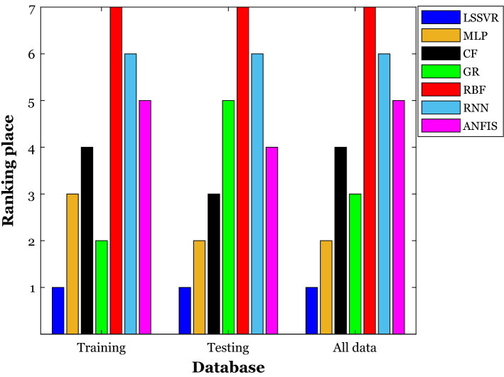
Although all these prediction accuracies confirm a high level of consistency with the laboratory-measured density, the LSSVR and RBF neural network present the highest and lowest precise results, respectively. For systematical approving this claim, the subsequent analysis has ranked these selected intelligent models based on their prediction accuracy in different stages of model development.
Selecting the best intelligent model using the ranking analysis
The ranking analysis is a well-established procedure to arrange several models based on their performance. The previous step measured the prediction ability of the seven selected intelligent models using five well-known statistical indexes. Now the ranking analysis utilizes the numerical values of these statistical indexes to arrange them from the best to the worst model. Equation (22) indicates that the selected models have been ranked based on their average rankings over five statistical criteria (indx).
| 22 |
This ranking analysis has been separately applied to the model’s performances during the learning and testing stages. Furthermore, the rank orders of the chosen intelligent models have also been tracked over the whole 1239 datasets. Figure 1 displays the rank order of the LSSVR, artificial neural network models (i.e., MLP, RNN, RBF, CFF, and GR), and ANFIS over three different databases. It can be easily inferred that the LSSVR with the three first ranking places and the RBF neural network with the three seventh ranking places are the best and worst tools for calculating the density of deep eutectic solvents. The ranking order of other constructed models has also displayed in this figure.
Figure 1.
The ranking order of the intelligent estimators in different stages of the model development.
In summary, it can be claimed that the LSSVR equipped with the Gaussian kernel function is the most trustful model for calculating the density of deep eutectic solvents from temperature and inherent characteristics (i.e., ω, Tc, and Pc) of the involved substance. This highly accurate model anticipates the density of 1239 deep eutectic solvents with the MAPE = 0.26%, MAE = 2.94, RAPE = 4.06%, RMSE = 5.65, and R2 = 0.99798.
Validation stage
The LSSVR versus empirical correlations
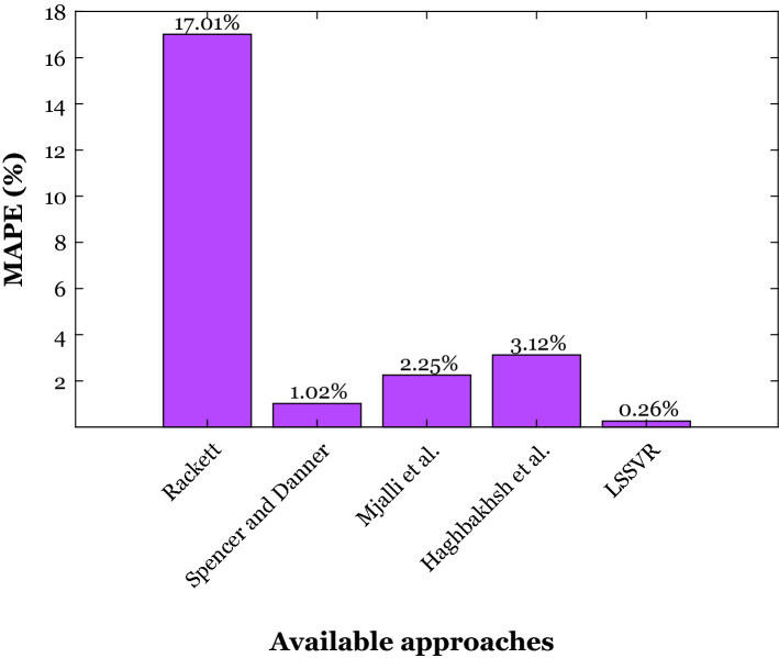
The accuracy of the suggested LSSVR and four empirical correlations in the literature (Rackett, Spencer and Danner, Mjalli et al., and Haghbakhsh et al.) for estimating 1239 densities of the deep eutectic solvent has been compared in the current section. The results of this comparison utilizing the MAPE have been described in Fig. 2. The observed results confirm that the LSSVR is the most accurate tool for estimating the density of deep eutectic solvents. The LSSVR anticipates 1239 density samples of 149 deep eutectic solvents with the MAPE = 0.26%, while the most accurate empirical correlation (Spencer and Danner model) presents the MAPE = 1.02% for an entirely similar database. The suggested LSSVR improves the best previously achieved accuracy by more than 74%.
Figure 2.
The prediction accuracy of the LSSVR and four empirical correlations in the literature28 to estimate the DES’s density of a completely similar database.
Validation using graphical inspections
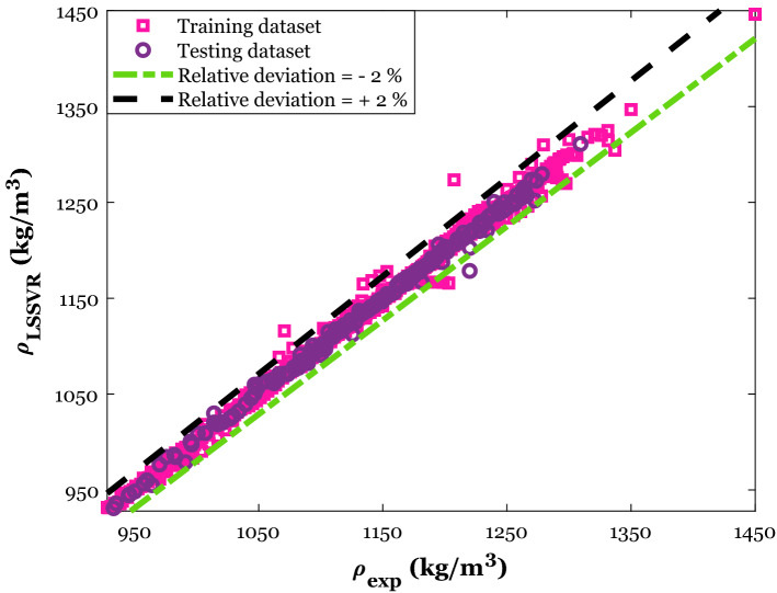
The anticipated densities by the LSSVR () versus their counterpart experimental values (i.e., cross-plot) have been shown in Fig. 3. This cross-plot separately presents the LSSVR predictions for both learning and testing steps. Two straight lines associated with the relative deviation percent (RD%) of − 2% and + 2% have also been added to this figure. Equation (23) expresses the formula of the RD%.
| 23 |
Figure 3.
The consistency between experimental values of DES’s density and the LSSVR’s prediction.
Figure 3 displays that about ten density samples have been anticipated with the RD% of lower than − 2% and higher than + 2%. The excellent ability of the built LSSVR to estimate the density of deep eutectic solvents can be readily approved by this observation.
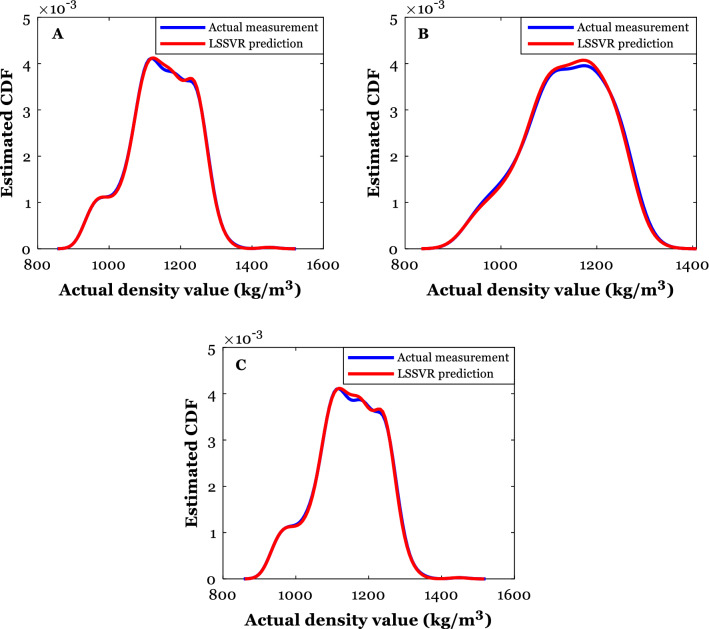
The kernel density estimation is a reliable method for visually inspecting the compatibility between a given variable’s actual and anticipated values. As Fig. 4 shows, this method depicts the cumulative distribution function (CDF) as a function of the experimental values of a given variable. Figure 4A–C illustrate the compatibility between actual and anticipated density values over the training and testing subdivisions and the whole database. Excluding the intermediate values of the DES’s density, a remarkable consistency can be seen between actual and predicted values. Moreover, it can be detected that both the experimental data and the LSSVR predictions have a standard Gaussian distribution shape.
Figure 4.
Utilizing the kernel density estimation method to check the LSSVR validity in the training (A) and testing (B) stages and against whole the databank (C).
The magnitude of difference between actual and predicted densities (the residual error, i.e., RE) is another statistical index applied to monitor the prediction accuracy of the built LSSVER. The mathematical expression of the RE is given in Eq. (24).
| 24 |
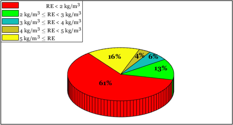
Based on reported results in Fig. 5, 61% of the available samples have been estimated with a residual error of less than 2 kg/m3. Moreover, the LSSVR successfully anticipated 84% of the experimental databank with an RE of lower than 5 kg/m3. Only 16% of the gathered database has been estimated with a residual error of higher than 5 kg/m3. All these observations confirm the excellent compatibility between calculated densities by the LSSVR and their related actual measurements.
Figure 5.
The cumulative frequency of the residual error (RE) of the LSSVR for estimating the DES’s density.
Checking the reliability of the gathered database
The gathered experimental data had a central role during the development/validation/selection of machine learning methods hereinbefore. Furthermore, this experimental databank has been used to compare the accuracy of empirical correlations and the selected LSSVR. The entire previous findings are valid only if the gathered laboratory-measured densities have an acceptable validity level. The leverage is a well-trusted technique to detect both valid and outlier data in an experimentally-measured database94. This technique plots the standardized residuals (SR) against the Hat index to accomplish its duty89. Equation (27) explains that the SR can be obtained by dividing the average value () and standard deviation (SD) of the residual error. Equations (25) and (26) give the and SD formula, respectively.
| 25 |
| 26 |
| 27 |
Furthermore, numerical values of the Hat index (HI) can be reached by applying Eq. (28) on the matrix of the independent variables ()95. The superscripts of T and -1 stand for the transpose and inverse operations, respectively.
| 28 |
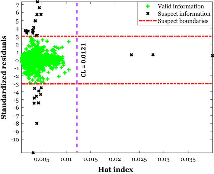
Figure 6 shows the plot of SR versus the HI values associated with the DES’s density databank. The leverage method states that the region bounded by the -3 < SR < + 3 and HI lower than the critical leverage is valid, and all other positions are the suspect domain96. Equation (29) helps calculate the critical leverage (CL) from the number of independent variables (NIV) and experimental data points (n)83,95. Having four independent variables and 1239 data points, the CL equals 0.0121.
| 29 |
Figure 6.
The results of applying the leverage method on the gathered density databank.
The leverage method approves that 1210 out of 1239 data points have appeared in the valid zone, and only 29 density samples may be outlier measurements. It can be claimed that the validity of the gathered database has been approved now, and all previous findings based on this databank are trustful.
LSSVR accuracy for density predicting each deep eutectic solvent
It may be a good idea to monitor the prediction accuracy of the LSSVR against the deep eutectic solvents with the same HBA agent. Since the average relative deviation (Eq. 30)97 clarifies both underestimated and overestimated predictions, it has been selected to measure the LSSVR accuracy in this stage.
| 30 |
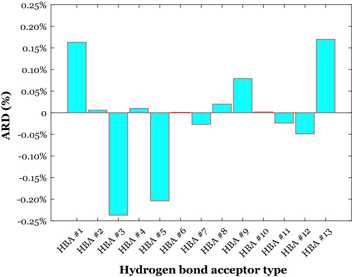
Figure 7 states that the density of thirteen classes of the deep eutectic solvent with the HBA#1 to HBA#13 (see Table 1) has been estimated with the ARD ranges from − 0.24 to + 0.17%. Those deep eutectic solvents having the HBA #1, 9, and 13 have been underestimated by the LSSVR. On the other hand, the DESs with the HBA #3, 5, and 12 have been overestimated. The ARD% associated with the other deep eutectic solvent classes is almost equal to zero.
Figure 7.
The observed average relative deviation between actual and predicted densities of the deep eutectic solvent with the same HBA agent.
Investigating the effect of temperature, and HBD/HBA types
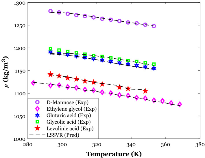
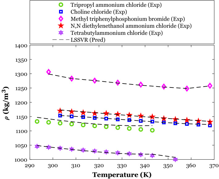
The effect of temperature on the density of deep eutectic solvents with the specific HBA agent (i.e., Choline chloride) and different HBD substances can be deduced from Fig. 8. This figure reports both experimentally-measured densities and their counterparts simulated values by the LSSVR. This figure readily justifies an excellent agreement between experimental and predicted density values. The LSSVR effectively discriminates between the effect of HBD type and working temperature on the density of the Choline chloride-based DESs and accurately estimates all distinct data points. Like the conventional liquid, the density of deep eutectic solvents decreases by increasing the working temperature. Increasing the intermolecular void volume in the DES’s body by increasing the temperature has been introduced as responsible for this observation98.
Figure 8.
The excellent performance of the LSSVR model for correctly identifying the HBD effect on the density of Choline chloride as an HBA.
The density variation of deep eutectic solvents with the temperature and HBA type has been exhibited in Fig. 9. All DESs in this analysis have glycerol as their HBD agent. A high level of compatibility between actual density values and their counterparts estimated by the LSSVR can be seen in Fig. 9. The LSSVR distinguishes the effect of HBA type and temperature on the DES’s density and accurately anticipates all individual density data points.
Figure 9.
Monitoring the ability of the LSSVR model to anticipate the HBA effect on the density of the glycerol as an HBD.
Simple flowchart of our study
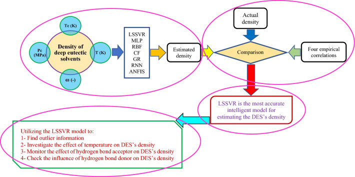
A simple and understandable flowchart for the stages followed in the current research study has been presented in Fig. 10. This figure can be broken down into four distinct parts as follows:
Developing machine learning methods
Comparing accuracy performances of the machine learning methods and empirical correlations
Selecting the model with the highest prediction accuracy
Utilizing the model chosen for further analyzing purposes
Figure 10.
A simple flowchart for explaining the stages followed in the present study.
Conclusion
The accuracy of seven machine learning methods and four empirical correlations has been compared to find the highest accurate tool for estimating the density of 149 deep eutectic solvents. Huge performed statistical analyses proved that the least-squares support vector regression equipped with the Gaussian kernel function is more accurate than the other methods investigated. This suggested scheme predicted 1239 experimentally-measured densities with the MAPE = 0.26%, MAE = 2.94, RAPE = 4.06%, RMSE = 5.65, and R2 = 0.99798. Visual inspections utilizing the cross-plot, kernel density estimation, residual error, and average relative deviation have also justified a high level of compatibility between LSSVR predictions and their experimentally-measured counterparts. Investigating the experimental database employing the leverage technique resulted in founding 1210 valid and 29 suspect information. Furthermore, the fabricated LSSVR successfully infers the effect of temperature and HBA and HBD types on the density of the deep eutectic solvent. The current research may be viewed as an initiative towards constructing reliable models for anticipating DESs properties. Such a model promotes an efficient solvent synthesis that can help design and simulate new processes utilizing the DES.
Supplementary Information
Author contributions
All authors have equally engaged in this research article.
Data availability
All data generated or analyzed during this study are included in the supplementary file.
Competing interests
The authors declare no competing interests.
Footnotes
Publisher's note
Springer Nature remains neutral with regard to jurisdictional claims in published maps and institutional affiliations.
Supplementary Information
The online version contains supplementary material available at 10.1038/s41598-022-08842-5.
References
- 1.Pianko-Oprych P, Hosseini SM, Jaworski Z. Model development of integrated CPOx reformer and SOFC stack system. Polish J. Chem. Technol. 2016;18:41–46. [Google Scholar]
- 2.Seaberg J, Kaabipour S, Hemmati S, Ramsey JD. A rapid millifluidic synthesis of tunable polymer-protein nanoparticles. Eur. J. Pharm. Biopharm. 2020;154:127–135. doi: 10.1016/j.ejpb.2020.07.006. [DOI] [PubMed] [Google Scholar]
- 3.Vaferi B, Bahmani M, Keshavarz P, Mowla D. Experimental and theoretical analysis of the UV/H2O2 advanced oxidation processes treating aromatic hydrocarbons and MTBE from contaminated synthetic wastewaters. J. Environ. Chem. Eng. 2014;2:1252–1260. [Google Scholar]
- 4.GhanbariPakdehi S, Vaferi B. A study on adsorptive removal of DMAZ from aqueous solutions by ZSM-5, NaY zeolites, and activated carbon: kinetic and isotherm. Desalin. Water Treat. 2016;57:18286–18292. [Google Scholar]
- 5.Jahanmahin O, Rahmati MMM, Mohammadi T, Babaee J, Khosravi A. Cr (VI) ion removal from artificial waste water using supported liquid membrane. Chem. Pap. 2016;70:913–925. [Google Scholar]
- 6.Rahimpour MR, Mazinani S, Vaferi B, Baktash MS. Comparison of two different flow types on CO removal along a two-stage hydrogen permselective membrane reactor for methanol synthesis. Appl. Energy. 2011;88:41–51. [Google Scholar]
- 7.P.C. Wankat, Separation process engineering: includes mass transfer (2012).
- 8.Anastas PT, Warner JC. Green chemistry. Front. (Boulder). 1998;640:1998. [Google Scholar]
- 9.Lashkarbolooki M, Vaferi B, Shariati A, Zeinolabedini Hezave A. Investigating vapor-liquid equilibria of binary mixtures containing supercritical or near-critical carbon dioxide and a cyclic compound using cascade neural network. Fluid Phase Equilib. 2013;343:24–29. [Google Scholar]
- 10.Rasool MA, Vankelecom IFJ. Use of γ-valerolactone and glycerol derivatives as bio-based renewable solvents for membrane preparation. Green Chem. 2019;21:1054–1064. [Google Scholar]
- 11.Chen J, Spear SK, Huddleston JG, Rogers RD. Polyethylene glycol and solutions of polyethylene glycol as green reaction media. Green Chem. 2005;7:64–82. [Google Scholar]
- 12.Valderrama JO, Sanga WW, Lazzús JA. Critical properties, normal boiling temperature, and acentric factor of another 200 ionic liquids. Ind. Eng. Chem. Res. 2008;47:1318–1330. [Google Scholar]
- 13.Deng D, Liu X, Gao B. Physicochemical properties and investigation of azole-based deep eutectic solvents as efficient and reversible SO2 absorbents. Ind. Eng. Chem. Res. 2017;56:13850–13856. [Google Scholar]
- 14.Florindo C, Oliveira MM, Branco LC, Marrucho IM. Carbohydrates-based deep eutectic solvents: thermophysical properties and rice straw dissolution. J. Mol. Liq. 2017;247:441–447. [Google Scholar]
- 15.Liu X, Gao B, Jiang Y, Ai N, Deng D. Solubilities and thermodynamic properties of carbon dioxide in guaiacol-based deep eutectic solvents. J. Chem. Eng. Data. 2017;62:1448–1455. [Google Scholar]
- 16.Li G, Jiang Y, Liu X, Deng D. New levulinic acid-based deep eutectic solvents: synthesis and physicochemical property determination. J. Mol. Liq. 2016;222:201–207. [Google Scholar]
- 17.Ghaedi H, Ayoub M, Sufian S, Lal B, Shariff AM. Measurement and correlation of physicochemical properties of phosphonium-based deep eutectic solvents at several temperatures (293.15 K–343.15 K) for CO2 capture. J. Chem. Thermodyn. 2017;113:41–51. [Google Scholar]
- 18.Carriazo D, Serrano MC, Gutiérrez MC, Ferrer ML, del Monte F. Deep-eutectic solvents playing multiple roles in the synthesis of polymers and related materials. Chem. Soc. Rev. 2012;41:4996–5014. doi: 10.1039/c2cs15353j. [DOI] [PubMed] [Google Scholar]
- 19.Zhao B-Y, Xu P, Yang F-X, Wu H, Zong M-H, Lou W-Y. Biocompatible deep eutectic solvents based on choline chloride: characterization and application to the extraction of rutin from Sophora japonica. ACS Sustain. Chem. Eng. 2015;3:2746–2755. [Google Scholar]
- 20.Mbous YP, Hayyan M, Hayyan A, Wong WF, Hashim MA, Looi CY. Applications of deep eutectic solvents in biotechnology and bioengineering: promises and challenges. Biotechnol. Adv. 2017;35:105–134. doi: 10.1016/j.biotechadv.2016.11.006. [DOI] [PubMed] [Google Scholar]
- 21.Emami S, Shayanfar A. Deep eutectic solvents for pharmaceutical formulation and drug delivery applications. Pharm. Dev. Technol. 2020;25:779–796. doi: 10.1080/10837450.2020.1735414. [DOI] [PubMed] [Google Scholar]
- 22.Ghaedi H, Ayoub M, Sufian S, Shariff AM, Murshid G, Hailegiorgis SM, Khan SN. Density, excess and limiting properties of (water and deep eutectic solvent) systems at temperatures from 293.15 K to 343.15 K. J. Mol. Liq. 2017;248:378–390. [Google Scholar]
- 23.Taherzadeh M, Haghbakhsh R, Duarte ARC, Raeissi S. Estimation of the heat capacities of deep eutectic solvents. J. Mol. Liq. 2020;307:112940. [Google Scholar]
- 24.Mahmoodi F, Darvishi P, Vaferi B. Prediction of coefficients of the Langmuir adsorption isotherm using various artificial intelligence (AI) techniques. J. Iran. Chem. Soc. 2018;15:2747–2757. [Google Scholar]
- 25.Karimi M, Aminzadehsarikhanbeglou E, Vaferi B. Robust intelligent topology for estimation of heat capacity of biochar pyrolysis residues. Measurement. 2021;183:109857. [Google Scholar]
- 26.Privat R, Moine E, Sirjean B, Gani R, Jaubert J-N. Application of the corresponding-state law to the parametrization of statistical associating fluid theory (SAFT)-type models: generation and use of “generalized charts”. Ind. Eng. Chem. Res. 2019;58:9127–9139. [Google Scholar]
- 27.He S, Guo F, Zou Q, Ding H. MRMD2.0: A python tool for machine learning with feature ranking and reduction. Curr. Bioinform. 2020;15:1–9. [Google Scholar]
- 28.Haghbakhsh R, Bardool R, Bakhtyari A, Duarte ARC, Raeissi S. Simple and global correlation for the densities of deep eutectic solvents. J. Mol. Liq. 2019;296:111830. [Google Scholar]
- 29.Knapp, H., Zeck, S., & Langhorst, R. Vapor-liquid equilibria for mixtures of low boiling substances. Pt. 3. Ternary systems (1989).
- 30.Basaiahgari A, Panda S, Gardas RL. Acoustic, volumetric, transport, optical and rheological properties of Benzyltripropylammonium based deep eutectic solvents. Fluid Phase Equilib. 2017;448:41–49. [Google Scholar]
- 31.Sánchez PB, González B, Salgado J, Parajó JJ, Domínguez Á. Physical properties of seven deep eutectic solvents based on l-proline or betaine. J. Chem. Thermodyn. 2019;131:517–523. [Google Scholar]
- 32.Yadav A, Kar JR, Verma M, Naqvi S, Pandey S. Densities of aqueous mixtures of (choline chloride+ ethylene glycol) and (choline chloride+ malonic acid) deep eutectic solvents in temperature range 283.15–363.15 K. Thermochim. Acta. 2015;600:95–101. [Google Scholar]
- 33.Harifi-Mood AR, Buchner R. Density, viscosity, and conductivity of choline chloride+ ethylene glycol as a deep eutectic solvent and its binary mixtures with dimethyl sulfoxide. J. Mol. Liq. 2017;225:689–695. [Google Scholar]
- 34.Florindo C, Oliveira FS, Rebelo LPN, Fernandes AM, Marrucho IM. Insights into the synthesis and properties of deep eutectic solvents based on cholinium chloride and carboxylic acids. ACS Sustain. Chem. Eng. 2014;2:2416–2425. [Google Scholar]
- 35.Yadav A, Trivedi S, Rai R, Pandey S. Densities and dynamic viscosities of (choline chloride+ glycerol) deep eutectic solvent and its aqueous mixtures in the temperature range (283.15–363.15) K. Fluid Phase Equilib. 2014;367:135–142. [Google Scholar]
- 36.Lu M, Han G, Jiang Y, Zhang X, Deng D, Ai N. Solubilities of carbon dioxide in the eutectic mixture of levulinic acid (or furfuryl alcohol) and choline chloride. J. Chem. Thermodyn. 2015;88:72–77. [Google Scholar]
- 37.Guo W, Hou Y, Ren S, Tian S, Wu W. Formation of deep eutectic solvents by phenols and choline chloride and their physical properties. J. Chem. Eng. Data. 2013;58:866–872. [Google Scholar]
- 38.Zhu J, Yu K, Zhu Y, Zhu R, Ye F, Song N, Xu Y. Physicochemical properties of deep eutectic solvents formed by choline chloride and phenolic compounds at T=(293.15 to 333.15) K: The influence of electronic effect of substitution group. J. Mol. Liq. 2017;232:182–187. [Google Scholar]
- 39.Yadav A, Pandey S. Densities and viscosities of (choline chloride+ urea) deep eutectic solvent and its aqueous mixtures in the temperature range 293.15 K to 363.15 K. J. Chem. Eng. Data. 2014;59:2221–2229. [Google Scholar]
- 40.Chemat F, Anjum H, Shariff AM, Kumar P, Murugesan T. Thermal and physical properties of (Choline chloride+ urea+ l-arginine) deep eutectic solvents. J. Mol. Liq. 2016;218:301–308. [Google Scholar]
- 41.Haghbakhsh R, Raeissi S. Densities and volumetric properties of (choline chloride+ urea) deep eutectic solvent and methanol mixtures in the temperature range of 293.15–323.15 K. J. Chem. Thermodyn. 2018;124:10–20. [Google Scholar]
- 42.Haghbakhsh R, Raeissi S. Investigation of solutions of ethyl alcohol and the deep eutectic solvent of Reline for their volumetric properties. Fluid Phase Equilib. 2018;472:39–47. [Google Scholar]
- 43.Chen Y, Ai N, Li G, Shan H, Cui Y, Deng D. Solubilities of carbon dioxide in eutectic mixtures of choline chloride and dihydric alcohols. J. Chem. Eng. Data. 2014;59:1247–1253. [Google Scholar]
- 44.Craveiro R, Aroso I, Flammia V, Carvalho T, Viciosa MT, Dionísio M, Barreiros S, Reis RL, Duarte ARC, Paiva A. Properties and thermal behavior of natural deep eutectic solvents. J. Mol. Liq. 2016;215:534–540. [Google Scholar]
- 45.Hayyan A, Mjalli FS, AlNashef IM, Al-Wahaibi T, Al-Wahaibi YM, Hashim MA. Fruit sugar-based deep eutectic solvents and their physical properties. Thermochim. Acta. 2012;541:70–75. [Google Scholar]
- 46.Mjalli FS, Ahmad O. Density of aqueous choline chloride-based ionic liquids analogues. Thermochim. Acta. 2017;647:8–14. [Google Scholar]
- 47.Shahbaz K, Baroutian S, Mjalli FS, Hashim MA, AlNashef IM. Densities of ammonium and phosphonium based deep eutectic solvents: prediction using artificial intelligence and group contribution techniques. Thermochim. Acta. 2012;527:59–66. [Google Scholar]
- 48.Leron RB, Soriano AN, Li MH. Densities and refractive indices of the deep eutectic solvents (choline chloride+ ethylene glycol or glycerol) and their aqueous mixtures at the temperature ranging from 298.15 to 333.15 K. J. Taiwan Inst. Chem. Eng. 2012;43:551–557. [Google Scholar]
- 49.Kareem MA, Mjalli FS, Hashim MA, AlNashef IM. Phosphonium-based ionic liquids analogues and their physical properties. J. Chem. Eng. Data. 2010;55:4632–4637. [Google Scholar]
- 50.Mjalli FS, Naser J, Jibril B, Alizadeh V, Gano Z. Tetrabutylammonium chloride based ionic liquid analogues and their physical properties. J. Chem. Eng. Data. 2014;59:2242–2251. [Google Scholar]
- 51.Su H-Z, Yin JM, Liu QS, Li CP. Properties of four deep eutectic solvents: density, electrical conductivity, dynamic viscosity and refractive index. Acta Phys. Chim. Sin. 2015;31:1468–1473. [Google Scholar]
- 52.Rodriguez NR, Requejo PF, Kroon MC. Aliphatic–aromatic separation using deep eutectic solvents as extracting agents. Ind. Eng. Chem. Res. 2015;54:11404–11412. [Google Scholar]
- 53.Cardellini F, Tiecco M, Germani R, Cardinali G, Corte L, Roscini L, Spreti N. Novel zwitterionic deep eutectic solvents from trimethylglycine and carboxylic acids: characterization of their properties and their toxicity. RSC Adv. 2014;4:55990–56002. [Google Scholar]
- 54.Rackett HG. Equation of state for saturated liquids. J. Chem. Eng. Data. 1970;15:514–517. [Google Scholar]
- 55.Shahbaz K, Mjalli FS, Hashim MA, AlNashef IM. Prediction of deep eutectic solvents densities at different temperatures. Thermochim. Acta. 2011;515:67–72. [Google Scholar]
- 56.Spencer CF, Danner RP. Improved equation for prediction of saturated liquid density. J. Chem. Eng. Data. 1972;17:236–241. [Google Scholar]
- 57.Mjalli FS, Shahbaz K, AlNashef IM. Modified Rackett equation for modelling the molar volume of deep eutectic solvents. Thermochim. Acta. 2015;614:185–190. [Google Scholar]
- 58.Li B, Feng Y, Xiong Z, Yang W, Liu G. Research on AI security enhanced encryption algorithm of autonomous IoT systems. Inf. Sci. (NY) 2021;575:379–398. [Google Scholar]
- 59.He Y, Dai L, Zhang H. Multi-branch deep residual learning for clustering and beamforming in user-centric network. IEEE Commun. Lett. 2020;24:2221–2225. [Google Scholar]
- 60.Meng F, Cheng W, Wang J. Semi-supervised software defect prediction model based on tri-training. KSII Trans. Internet Inf. Syst. 2021;15:4028–4042. [Google Scholar]
- 61.Wang Y, Wang H, Zhou B, Fu H. Multi-dimensional prediction method based on Bi-LSTMC for ship roll. Ocean Eng. 2021;242:110106. [Google Scholar]
- 62.Liu F, Zhang G, Lu J. Heterogeneous domain adaptation: An unsupervised approach. IEEE Trans. Neural Netw. Learn. Syst. 2020;31:5588–5602. doi: 10.1109/TNNLS.2020.2973293. [DOI] [PubMed] [Google Scholar]
- 63.Ma Z, Zheng W, Chen X, Yin L. Joint embedding VQA model based on dynamic word vector. PeerJ Comput. Sci. 2021;7:e353. doi: 10.7717/peerj-cs.353. [DOI] [PMC free article] [PubMed] [Google Scholar]
- 64.Nabavi M, Nazarpour V, Alibak AH, Bagherzadeh A, Alizadeh SM. Smart tracking of the influence of alumina nanoparticles on the thermal coefficient of nanosuspensions: application of LS-SVM methodology. Appl. Nanosci. 2021;11:2113–2128. [Google Scholar]
- 65.Esmaeili-Faraj SH, Vaferi B, Bolhasani A, Karamian S, Hosseini S, Rashedi R. Design a neuro-based computing paradigm for simulating of industrial olefin plants. Chem. Eng. Technol. 2021;44:1382–1389. [Google Scholar]
- 66.Mousavi NS, Romero-Martínez A, Ramírez-Verduzco LF. Predicting the surface tension of mixtures of fatty acid ethyl esters and biodiesel fuels using UNIFAC activity coefficients. Fluid Phase Equilib. 2020;507:112430. [Google Scholar]
- 67.Moghimihanjani M, Vaferi B. A combined wavelet transform and recurrent neural networks scheme for identification of hydrocarbon reservoir systems from well testing signals. ASME J. Energy Resour. Technol. Energy Resour. Technol. Energy Resour. Technol. 2021;143:13001. [Google Scholar]
- 68.Jafari Gukeh M, Moitra S, Ibrahim AN, Derrible S, Megaridis CM. Machine learning prediction of TiO2-coating wettability tuned via UV exposure. ACS Appl. Mater. Interf. 2021;13:46171–46179. doi: 10.1021/acsami.1c13262. [DOI] [PubMed] [Google Scholar]
- 69.Zhang Z, Tian J, Huang W, Yin L, Zheng W, Liu S. A haze prediction method based on one-dimensional convolutional neural network. Atmosphere (Basel). 2021;12:1327. [Google Scholar]
- 70.Khalifeh A, Vaferi B. Intelligent assessment of effect of aggregation on thermal conductivity of nanofluids-Comparison by experimental data and empirical correlations. Thermochim. Acta. 2019;681:178377. [Google Scholar]
- 71.Liu, Z. et al. Investigating pose representations and motion contexts modeling for 3D motion prediction. In: IEEE Transactions on Pattern Analysis and Machine Intelligence, IEEE. 10.1109/TPAMI.2021.3139918 (2020). [DOI] [PubMed]
- 72.Vaferi B, Eslamloueyan R, Ayatollahi S. Application of recurrent networks to classification of oil reservoir models in well-testing analysis. Energy Sour. A Recover. Util. Environ. Eff. 2015;37:174–180. [Google Scholar]
- 73.Shang K, Chen Z, Liu Z, Song L, Zheng W, Yang B, Liu S, Yin L. Haze prediction model using deep recurrent neural network. Atmosphere (Basel). 2021;12:1625. [Google Scholar]
- 74.Rooki R. Application of general regression neural network (GRNN) for indirect measuring pressure loss of Herschel-Bulkley drilling fluids in oil drilling. Measurement. 2016;85:184–191. [Google Scholar]
- 75.Hagan, M.T., Demuth, H.B., & Beale, M. Neural network design. PWS Publishing Co., 1997.
- 76.Mousavi NS, Vaferi B, Romero-Martínez A. Prediction of surface tension of various aqueous amine solutions using the UNIFAC model and artificial neural networks. Ind. Eng. Chem. Res. 2021;60:10354–10364. [Google Scholar]
- 77.Wang Y, Zou R, Liu F, Zhang L, Liu Q. A review of wind speed and wind power forecasting with deep neural networks. Appl. Energy. 2021;304:117766. [Google Scholar]
- 78.Dizadji, M.R., Yousefi-Koma, A., & Gharehnazifam, Z. 3-Axis attitude control of satellite using adaptive direct fuzzy controller. In: Proceedings of the 2018 6th RSI International Conferences on Robotics Mechatronics, IEEE, 2018: pp. 1–5.
- 79.Dizaji, M.R., Yazdi, M.R.H., Shirzi, M.A., & Gharehnazifam, Z., Fuzzy supervisory assisted impedance control to reduce collision impact. In: Proceedings of the 2014 Second RSI/ISM International Conference on Robotics Mechatronics, IEEE, 2014: pp. 858–863.
- 80.Zamani HA, Rafiee-Taghanaki S, Karimi M, Arabloo M, Dadashi A. Implementing ANFIS for prediction of reservoir oil solution gas-oil ratio. J. Nat. Gas Sci. Eng. 2015;25:325–334. [Google Scholar]
- 81.Motahari-Nezhad M, Jafari SM. ANFIS system for prognosis of dynamometer high-speed ball bearing based on frequency domain acoustic emission signals. Measurement. 2020;166:108154. [Google Scholar]
- 82.Shojaei M-J, Bahrami E, Barati P, Riahi S. Adaptive neuro-fuzzy approach for reservoir oil bubble point pressure estimation. J. Nat. Gas Sci. Eng. 2014;20:214–220. [Google Scholar]
- 83.Cao Y, Kamrani E, Mirzaei S, Khandakar A, Vaferi B. Electrical efficiency of the photovoltaic/thermal collectors cooled by nanofluids: machine learning simulation and optimization by evolutionary algorithm. Energy Rep. 2022;8:24–36. [Google Scholar]
- 84.Seyed Alizadeh SM, Bagherzadeh A, Bahmani S, Nikzad A, Aminzadehsarikhanbeglou E, Tatyana Yu S. Retrograde gas condensate reservoirs: reliable estimation of dew point pressure by the hybrid neuro-fuzzy connectionist paradigm. J. Energy Resour. Technol. 2021;144:63007. [Google Scholar]
- 85.Daryayehsalameh B, Nabavi M, Vaferi B. Modeling of CO2 capture ability of [Bmim][BF4] ionic liquid using connectionist smart paradigms. Environ. Technol. Innov. 2021;22:101484. [Google Scholar]
- 86.Karimi M, Alibak AH, Alizadeh SMS, Sharif M, Vaferi B. Intelligent modeling for considering the effect of bio-source type and appearance shape on the biomass heat capacity. Measurement. 2021;189:110529. [Google Scholar]
- 87.Rehamnia I, Benlaoukli B, Jamei M, Karbasi M, Malik A. Simulation of seepage flow through embankment dam by using a novel extended Kalman filter based neural network paradigm: case study of Fontaine Gazelles Dam. Algeria. Measurement. 2021;176:109219. [Google Scholar]
- 88.Jiang Y, Zhang G, Wang J, Vaferi B. Hydrogen solubility in aromatic/cyclic compounds: Prediction by different machine learning techniques. Int. J. Hydrogen Energy. 2021;46:23591–23602. [Google Scholar]
- 89.Nabipour N, Qasem SN, Salwana E, Baghban A. Evolving LSSVM and ELM models to predict solubility of non-hydrocarbon gases in aqueous electrolyte systems. Measurement. 2020;164:107999. [Google Scholar]
- 90.Xie J, Liu X, Lao X, Vaferi B. Hydrogen solubility in furfural and furfuryl bio-alcohol: Comparison between the reliability of intelligent and thermodynamic models. Int. J. Hydrogen Energy. 2021;73:36056–36068. [Google Scholar]
- 91.Vaferi B, Eslamloueyan R, Ghaffarian N. Hydrocarbon reservoir model detection from pressure transient data using coupled artificial neural network-Wavelet transform approach. Appl. Soft Comput. J. 2016;47:63–75. [Google Scholar]
- 92.Karimi M, Vaferi B, Hosseini SH, Rasteh M. Designing an efficient artificial intelligent approach for estimation of hydrodynamic characteristics of tapered fluidized bed from its design and operating parameters. Ind. Eng. Chem. Res. 2018;57:259–267. [Google Scholar]
- 93.Ghanbari S, Vaferi B. Experimental and theoretical investigation of water removal from DMAZ liquid fuel by an adsorption process. Acta Astronaut. 2015;112:19–28. [Google Scholar]
- 94.Zhou Z, Davoudi E, Vaferi B. Monitoring the effect of surface functionalization on the CO2 capture by graphene oxide/methyl diethanolamine nanofluids. J. Environ. Chem. Eng. 2021;9:106202. [Google Scholar]
- 95.Moosavi SR, Vaferi B, Wood DA. Auto-characterization of naturally fractured reservoirs drilled by horizontal well using multi-output least squares support vector regression. Arab. J. Geosci. 2021;14:545. [Google Scholar]
- 96.Hosseini S, Vaferi B. Determination of methanol loss due to vaporization in gas hydrate inhibition process using intelligent connectionist paradigms. Arab. J. Sci. Eng. 2021 doi: 10.1007/s13369-021-05679-4. [DOI] [Google Scholar]
- 97.Yang, W. et al. A privacy-preserving aggregation scheme based on negative survey for vehicle fuel consumption data. Inf. Sci.570, 526–544. 10.1016/j.ins.2021.05.009 (2020).
- 98.Nowosielski B, Jamrógiewicz M, Łuczak J, Śmiechowski M, Warmińska D. Experimental and predicted physicochemical properties of monopropanolamine-based deep eutectic solvents. J. Mol. Liq. 2020;309:113110. [Google Scholar]
Associated Data
This section collects any data citations, data availability statements, or supplementary materials included in this article.
Supplementary Materials
Data Availability Statement
All data generated or analyzed during this study are included in the supplementary file.


