Abstract
Background
DCLEAR is an R package used for single cell lineage reconstruction. The advances of CRISPR-based gene editing technologies have enabled the prediction of cell lineage trees based on observed edited barcodes from each cell. However, the performance of existing reconstruction methods of cell lineage trees was not accessed until recently. In response to this problem, the Allen Institute hosted the Cell Lineage Reconstruction Dream Challenge in 2020 to crowdsource relevant knowledge from across the world. Our team won sub-challenges 2 and 3 in the challenge competition.
Results
The DCLEAR package contained the R codes, which was submitted in response to sub-challenges 2 and 3. Our method consists of two steps: (1) distance matrix estimation and (2) the tree reconstruction from the distance matrix. We proposed two novel methods for distance matrix estimation as outlined in the DCLEAR package. Using our method, we find that two of the more sophisticated distance methods display a substantially improved level of performance compared to the traditional Hamming distance method. DCLEAR is open source and freely available from R CRAN and from under the GNU General Public License, version 3.
Conclusions
DCLEAR is a powerful resource for single cell lineage reconstruction.
Keywords: Cell lineage tracing, Lineage reconstruction, Machine learning, Simulation
Background
A multicellular organism or animal develops from one to two to four to an exponential number of cells. One of the challenges is the ability to predict the lineage tree representing the cell differentiation process starting from the single parental cell, based on cells extracted from the adult body. McKenna et al. [1] used gene editing technology and the immune system (CRISPR-CAS9) as the basis for proposing a methodology called GESTALT for estimating a cell-level lineage tree using the data generated using CRISPR-CAS9 barcode edits from each cell. Subsequently, Raj et al. [2] proposed scGESTALT, which further considers cell type identification as an extension of GESTALT. Researchers have developed a number of additional CRISPR recorder-based technologies [3–5].
This field lacked experimentation or analyses regarding the effectiveness of these proposed algorithms for comprehensive evaluation. To improve the evaluation process, the Allen Institute established The Cell Lineage Reconstruction DREAM Challenge [6]. The Allen Institute proposed three different sub-challenges to benchmark reconstruction algorithms of cell lineage trees: (1) the reconstruction of in vitro cell lineages of 76 trees with fewer than 100 cells; (2) the reconstruction of an in silico cell lineage tree of 1000 cells; (3) the reconstruction of an in silico cell lineage tree of 10,000 cells. Our proposed DCLEAR method won sub-challenges 2 and 3 of this challenge competition.
We outline and define the problem setting addressed in cell lineage reconstruction in the next section. We then present two core methods for distance matrix construction and outline how DCLEAR software may be applied to a simulated dataset.
Implementation
Problem setup
Assume we have n number of training data pairs. Each data pair consists of a set of cell sequences and a true cell lineage tree. One example of such a pair is illustrated in Fig. 1.
Fig. 1.

a is the observed set of cell sequences, and b is the cell lineage tree. The goal is to predict the cell lineage tree in (b) using the cell sequences in (a)
For the ith data pair, let be the number of cell sequences in the ith data pair and let t be the sequence length. Let the sequence information in data pair i be written as , an matrix. The matrix element describes the jth sequence and the kth letter of the ith training data pair. Furthermore, we represent , the cell lineage tree structure, in the form of a Newick format string.
For example, if Fig. 1 represents ith data pair, (a) shows the sequence information. It has cell sequences, each sequence length has a length (t) of 10, and the first letter of the 3rd sequence is . The cell lineage tree is shown in Fig. 1b. In Newick format, .
We built our model () with n training pairs. The input matrix, C is an sequence information matrix. The output is the Newick format string representing the tree structure while represents the parameter set related to model , and represents the estimated parameter with n training data pairs.
To evaluate the model, we have l number of unused data. The loss is indicated as . The loss increases when the predicted tree structure () differs from the true tree structure (). We use the averaged loss metric (AL) defined below to evaluate the model .
| 1 |
Next, we need to define the quantity that represents the dissimilarity between the two lineage trees, and . The two widely used measures of this dissimilarity are the Robinson–Foulds (RF) distance [7] and the Triplet distance [8].
Figure 2 represents two lineage trees, and . The possible separations for tree 1 are and , and the possible separations for tree 2 are and . Among the four possible separations, in tree 1 and tree 2 are concordant separations. The RF distance is defined as the total number of concordant separations divided by the total number of separations. As an example: the RF score for Figure 2 is 2/4 = 0.5.
Fig. 2.
Two different trees, a and b , are presented to explain how the RF and triplet distances are defined. There are two possible cuts for each tree to separate items in the tree with two different sets of more than two items. The red slanted lines represent the possible cuts for separation
For triplet distance calculations, we sample three items among all items in the tree. We determine possible cases. We check whether the tree structure of the three items in tree 1 and tree 2 are the same. For example, the five cases of and have the same tree structure in both tree 1 and tree 2. The triplet score is defined as the number of cases with the same tree structure divided by the number of possible cases. Accordingly, the triplet score for our example is 5/10 = 0.5.
We will use to denote the RF distance and to denote the triplet distance.
Overview of the modeling architecture
The two main issues that need to be answered in the lineage reconstruction problem are (1) how should the model be built and (2) how should be estimated? Our modeling architecture for is described in Fig. 3. We divide the model into two parts: (1) estimating the distance between cells and (2) constructing a tree using a distance matrix. Let D(C) be a function for estimating the distance matrix for an input sequence matrix, C, and let t(D) be a function for predicting the lineage tree for an distance matrix, D. Note that a knowledge of the triangular components in D is sufficient for defining the distance matrix. Subsequently, the challenge becomes how and should be defined.
Fig. 3.
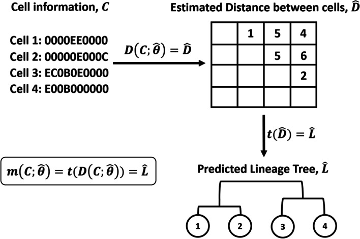
Overview of our modeling architecture. Our model function is divided into two parts: (1) estimating the distance between cells and (2) constructing a tree using the distance matrix
Choice of distance
One notion for calculating the distance is to define the distance function for the two sequences. Let be the calculated distance between the ith cell and the jth cell obtained from the given cell information matrix C. The quantities represent the ith cell vector taken from C. The quantity is the (i, j)th element of the cell distance matrix D. The next challenge becomes how should be defined.
Hamming distance method
One naive approach to modeling is to compute the Hamming distance expressed in equation (2):
| 2 |
where is an indicator function with a value of 1 if the given condition is true and 0 otherwise. Note that the Hamming distance simply counts unit differences between the two sequences and .
The simple calculation of the Hamming distance does not meet the challenges of the present study. Consider the cell differentiation process illustrated in Fig. 4. Let the 2nd and the 3rd leaf cells (dotted) have and . The corresponding Hamming distance is . However, it is not reasonable to assign equal weights to each target position. This deficiency is addressed by the weighted Hamming approach described in the following sub-sub-section.
Fig. 4.
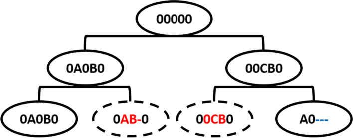
Example of cell differentiation process
The code for using the Hamming distance method is available from the phangorn package [9] using the dist.hamming function.
Weighted Hamming distance (WHD) method
An example of the cell diffusion process is illustrated in Fig. 4. Consider the objective of reconstructing the lineage tree based on information about the leaf nodes. What would be an appropriate measure for calculating the distance between 0AB-0 and 00CB0 (see the dotted circles in Fig. 4)? The character difference between ‘A’ and ‘0’ would be less than the character difference between ‘B’ and ‘C’ as the initial state ‘0’ can be differentiated to ‘A’ or to any other outcome states, whereas states ‘B’ and ‘C’ cannot be differentiated to other outcome states. In addition, the missing state ’-’ maybe any other state. Seeking a mathematical formula to accommodate these nuances, we propose the weighted Hamming distance (WHD) method:
| 3 |
where, is the lth character in the ith cell sequence, and is a weight associated with the character . The code for calculating the WHD method is available as the dist_weighted_hamming function in the DCLEAR package. For the estimation of weight parameters, we used Bayesian hyperparameter optimization using the BayesianOptimization function in the rBayesianOptimization package [10].
k-mer replacement distance (KRD) method
The algorithm used to compute the k-mer replacement distance (KRD) method first uses the prominence of mutations in the character arrays to estimate the summary statistics used for the generation of the tree to be reconstructed. These statistics include the mutation rate, the mutation probability for each character in the array, the number of targets, and the number of cells. These estimated parameters were combined with pre-defined parameters, such as the number of cell divisions, to simulate multiple lineage trees starting from the non-mutated root. To generate trees with sizes and mutation distributions similar to the target tree, we generated 1000 lineage trees, each with 16 cell divisions of 216 leaves, a mutation rate of 0.1, arrays of 200 characters, 200 cells, and 30 states (‘A’-‘Z’ to ‘a’-‘c’, with an outcome probability following a Gamma distribution with a shape of 0.1 and a rate of 2). Different possibilities for the k-mer distance method were then estimated from the simulated lineage trees and used to compute the distances between the input sequences in the character arrays of internal nodes and tips. The KRD method is available from the DCLEAR package using the dist_replacement function.
Tree construction
We use existing methods such as Neighbor-Joining (NJ), UPGMA, and FastMe [11–13] for tree construction from the estimated distance matrix, D. The NJ method is implemented as the nj function in the Analysis of Phylogenetics and Evolution (ape) package, UPGMA is implemented as the upgma function in the phangorn package, and FastMe is implemented as fastme.bal, and fastme.ols in the ape package.
Results
This section reports the experimental results of applying the Hamming distance, WHD, and KRD methods using existing tree construction methods (NJ, UPGMA, and FastMe). For the use of NJ, UPGMA, and FastMe, the nj function in the ape package [14] was used for the NJ method, the upgma function in the phangorn package [9] was used for the UPGMA method, the fastme.ols function in the ape was used for the FastMe method, and the fastme.bal function in the ape was used for FastMe with tree rearrangement.
Datasets
Simulation dataset
The simulation dataset was generated from our simulation code. Parameter settings for the simulation were as follows:
Number of targets: 50, 100, and 200
Mutation probability: 0.02, 0.04, 0.06, 0.08, and 0.1
Number of cells: 100
Dropout probability: 0, 0.05, and 0.1
Number of cell division: 16
Existance of point deletion: True, False
We iterated all 90 combinations () of the parameter 5 times, result in 450 simulation datasets. For each iteration, We generated five training sets and one evaluation set. The averaged performance of the 450 evaluation sets was reported.
Sub-challenge 2 and 3 datasets
The sub-challenge 2 and 3 datasets can be downloaded from the competition website of the Allen Institute Cell Lineage Reconstruction Challenge at https://www.synapse.org/#!Synapse:syn20692755 (accessed on 17 September 2021). The sub-challenge 2 dataset (the dataset for C.elegans cells) contained a 1000 cell tree from the 200 mutated/non-mutated targets in each cell induced by simulation, and the sub-challenge 3 dataset (the dataset for mouse cells) had a 10,000 cell tree from the 1000 mutated/non-mutated targets in each cell induced by simulation. The different simulation models were used for sub-challenges 2 and 3. Both datasets had 100 trees. We randomly divided the sub-challenge dataset into 75 trees for training and 25 trees for evaluation.
Experimental results
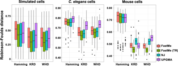
We outlined our experimental results in Fig. 5. The y-axis represented the RF distance, and the x-axis accommodated the different models. The Hamming distance, the KRD, and the WHD methods were used for distance calculation. NJ, UPGMA, and FastMe were methods for tree construction. For all three datasets, the KRD and the WHD methods displayed improved performance compared to the Hamming distance method. The performance achieved with the KRD was similar to that achieved with WHD. Among the tree construction methods, FastMe with tree rearrangement displayed improved performance compared to the other tree construction methods.
Fig. 5.
Experimental result
Discussion
In these experiments, we only compared the Hamming distance, the WHD, and the KRD methods using the three datasets. Gong et al. [6] presented the comparison of the WHD and the KRD with the other methods that participated in the Cell Lineage Reconstruction Dream Challenge (2020). Our proposed WHD method was used for sub-challenge 3, and the KRD method was used for sub-challenge 2. DCLEAR won both sub-challenges 2 and 3 but did not participate in sub-challenge 1. The sub-challenge 1 dataset has only ten target positions with two outcome states. The WHD and KRD methods were more powerful techniques with more complex settings, such as the existence of a dropout interval, the existence of missing target positions, and a larger number of outcome states. With the small target positions and the small outcome states of sub-challenge 1, the gain achieved by using the WHD and the KRD methods was not high. We were not able to show a comparison for sub-challenge 1 as DCLEAR did not participate in that sub-challenge. Thus, the future work of DCLEAR will contain an extension of the WHD and the KRD methods with small target and small outcome settings. Furthermore, for the WHD method, the hyperparameter tuning was performed using BayesianOptimization because the loss was not differentiable with respect to weight parameters. We could utilize the surrogate loss to address this non-differentiable loss [15].
Conclusions
DCLEAR is a powerful resource for single cell lineage reconstruction.
Abbreviations
- DCLEAR
Distance based Cell LinEAge Reconstruction
- CRISPR
Clustered regularly interspaced short palindromic repeats
- R
Statistical Language R
- CRAN
Comprehensive R archive network
- GESTALT
Genome editing of synthetic target arrays for lineage tracing
- scGESTALT
An extended version of GESTALT considering single-cell RNA sequencing data
- AL
Averaged loss metric
- RF
Robinson–Foulds distance
- WHD
Weighted Hamming distance
- KRD
k-mer replacement distance
- NJ
Neighbor-joining
- UPGMA
Unweighted pair group method with arithmetic mean
- FastMe
Fast distance-based phylogeny inference program
Appendix
Simulating trees with barcodes
For a simple illustration of lineage reconstruction, we simulated data using the sim_seqdata function in the DCLEAR package coded using the R [16] language. The sim_n parameter represented the number of cell samples. The prob_state parameter represented the cell state probability. The parameter m represented the number of targets. The parameter n_s represented the number of outcome states which equals the length quantified by prob_state. The parameter mu_d represented the mutation probability for each target position on every cell division. The parameter d represented the number of cell divisions. Finally, the parameter p_d represented the dropout probability of each target position for every cell division. The code is outlined below:
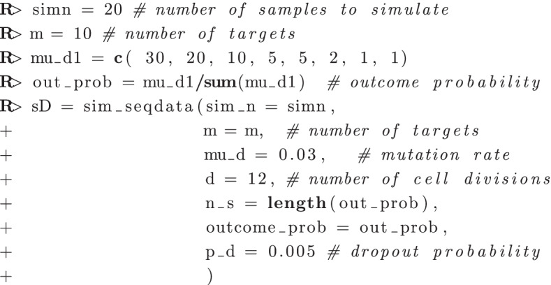
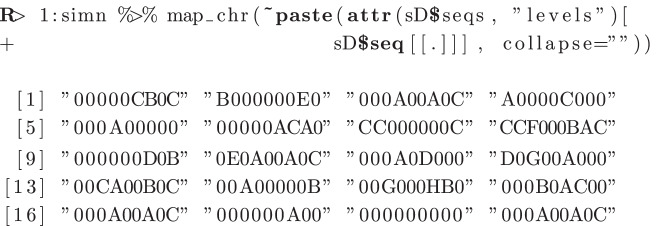
With this code, we generate a lineage tree of 20 leaf barcodes with 10 target positions. The sD$seqs contains the sequence information, and the sD$tree has the true tree structure:
We can also print character information of the simulated barcodes.
The initial cell state is ‘0000000000’. There are number of cell divisions resulting in leaf nodes. Every target position changes to a different outcome state for each cell division with a probability . The mutational positions randomly change to different outcomes, which follows a multinomial distribution with a probability . Every target position of leaf nodes randomly changes to a missing state (’-’) with a probability . Finally, cells are randomly sampled. The true lineage tree structure of 20 cells () is recorded in sD$tree. The tree structure corresponding to cells is illustrated in Fig. 6.
Fig. 6.
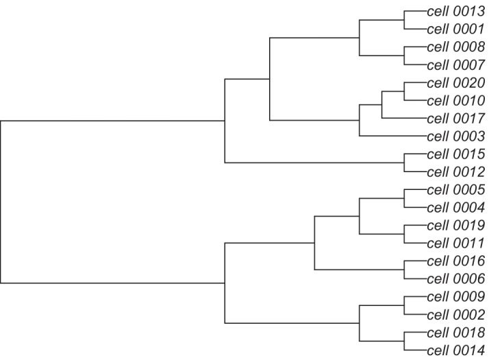
Tree structure of 20 leaf cells
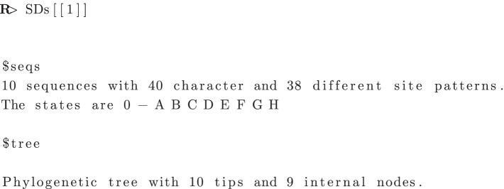
Subsequently, we prepared five lineage trees as a training dataset. Each lineage tree has 10 leaves with 40 barcode target positions:
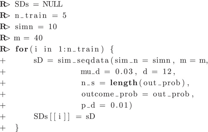
SDs is a list of 5 lineage trees. Each item of the SDs list is generated using sim_seqdata function:
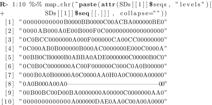
The ten barcodes of the first training data are shown below.
We observed interval missing (dropout) events by marking them with a sequence of hyphens. Weight parameters for the WHD method were trained using the WH_train function. We specified the weight for the initial state and the weight for the dropout state.
We printed out the state characters as indicated below:

Since the initial state (‘0’) is in the first position and the dropout state (‘-’) is in the second position, we specify loc0=1 and locDroputout = 2:
![]()
We simulated one evaluation datum and compared the ground truth tree with three generated trees using the Hamming, WHD, and KRD distances with the FastMe algorithm for tree construction:
First, we calculated the distance matrix using the Hamming distance, the WHD, and the KRD methods:
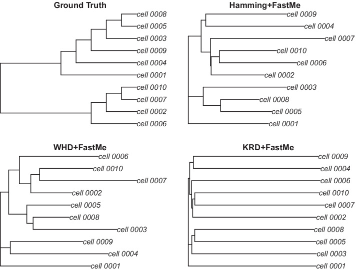
Second, we constructed the tree using the FastMe algorithm with the tree rearrangement using fastme.bal function. The ground truth tree and the three generated trees were demonstrated in Fig. 7. As an alternative to fastme.bal function, we could use different tree construction algorithms using nj, upgma, and fastme.ols functions.
Fig. 7.
Tree structure of 10 leaf cells, as determined for various standard distance measures
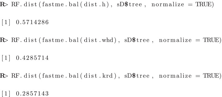
As outlined in Fig. 7, it is challenging to compare and determine which generation is the optimal one. One useful metric for making a determination is the RF distance. We calculated and compared the RF distances for the various generations. The RF distances were calculated and compared as indicated below:
The lower the value of the RF distance between the ground truth tree and the generated tree, the greater the similarity between the ground truth tree and the generated tree. Thus, for the given example data, the KRD method produced optimal results.
Authors’ contributions
IYK and WG participated in the design of the tool, implemented and tested the software, drafted the manuscript. HJK and DJG provided expert feedback in the design of the tool, the evaluation of the results and on the writing of the paper. All authors read and approved the final manuscript.
Funding
This work was supported by the National Research Foundation of Korea (NRF) grant funded by the Korea government (MSIP) (No. NRF-2020R1C1C1A01013020).
Availability of data and materials
DCLEAR is available from R cran at https://cran.r-project.org/web/packages/DCLEAR/index.html, and Github at https://github.com/ikwak2/DCLEAR Datasets are downlaodable from the challenge website, https://www.synapse.org/#!Synapse:syn20692755/wiki/. after agreeing the terms and conditions. The R/DCLEAR package is free software; you can redistribute it and/or modify it under the terms of the GNU General Public License, version 3.
Declarations
Ethics approval and consent to participate
Not applicable.
Competing interests
The authors declare that they have no competing interests.
Consent for publication
Not applicable.
Footnotes
Publisher's Note
Springer Nature remains neutral with regard to jurisdictional claims in published maps and institutional affiliations.
Contributor Information
Wuming Gong, Email: gongx030@umn.edu.
Hyunwoo J. Kim, Email: hyunwoojkim@korea.ac.kr
Daniel J. Garry, Email: garry@umn.edu
Il-Youp Kwak, Email: ikwak2@cau.ac.kr.
References
- 1.McKenna A, Findlay GM, Gagnon JA, Horwitz MS, Schier AF, Shendure J. Whole-organism lineage tracing by combinatorial and cumulative genome editing. Science. 2016;353:6298. doi: 10.1126/science.aaf7907. [DOI] [PMC free article] [PubMed] [Google Scholar]
- 2.Raj B, Wagner DE, McKenna A, Pandey S, Klein AM, Shendure J, Gagnon JA, Schier AF. Simultaneous single-cell profiling of lineages and cell types in the vertebrate brain. Nat Biotechnol. 2018;36(5):442–450. doi: 10.1038/nbt.4103. [DOI] [PMC free article] [PubMed] [Google Scholar]
- 3.Frieda KL, Linton JM, Hormoz S, Choi J, Chow K-HK, Singer ZS, Budde MW, Elowitz MB, Cai L. Synthetic recording and in situ readout of lineage information in single cells. Nature. 2017;541:107–111. doi: 10.1038/nature20777. [DOI] [PMC free article] [PubMed] [Google Scholar]
- 4.Alemany A, Florescu M, Baron CS, Peterson-Maduro J, van Oudenaarden A. Whole-organism clone tracing using single-cell sequencing. Nature. 2018;556:108–112. doi: 10.1038/nature25969. [DOI] [PubMed] [Google Scholar]
- 5.Jones MG, Khodaverdian A, Quinn JJ, Chan MM, Hussmann JA, Wang R, Xu C, Weissman JS, Yosef N. Inference of single-cell phylogenies from lineage tracing data using cassiopeia. Genome Biol. 2020;21(1):92. doi: 10.1186/s13059-020-02000-8. [DOI] [PMC free article] [PubMed] [Google Scholar]
- 6.Gong W, Granados AA, Hu J, Jones MG, Raz O, Salvador-Martínez I, Zhang H, Chow K-HK, Kwak I-Y, Retkute R, Prusokas A, Prusokas A, Khodaverdian A, Zhang R, Rao S, Wang R, Rennert P, Saipradeep VG, Sivadasan N, Rao A, Joseph T, Srinivasan R, Peng J, Han L, Shang X, Garry DJ, Yu T, Chung V, Mason M, Liu Z, Guan Y, Yosef N, Shendure J, Telford MJ, Shapiro E, Elowitz MB, Meyer P. Benchmarked approaches for reconstruction of in vitro cell lineages and in silico models of c. elegans and m. musculus developmental trees. Cell Syst. 2021. 10.1016/j.cels.2021.05.008 [DOI] [PubMed]
- 7.Robinson DF, Foulds LR. Comparison of phylogenetic trees. Math Biosci. 1981;53(1):131–147. [Google Scholar]
- 8.Dobson AJ. Comparing the shapes of trees. In: Street AP, Wallis WD, editors. Combinatorial mathematics III. Berlin: Springer; 1975. pp. 95–100. [Google Scholar]
- 9.Schliep K, Paradis E, Martins LdO, Potts A, White TW, Stachniss C, Kendall M, Halabi K, Bilderbeek R, Winchell K, Revell L, Gilchrist M, Beaulieu J, O’Meara B, Jackman LQ. Phangorn: Phylogenetic Reconstruction and Analysis. 2015. R package version 2.5.5. https://CRAN.R-project.org/package=phangorn
- 10.Yan Y. rBayesianOptimization: Bayesian Optimization of Hyperparameters. 2016. R package version 1.1.0. https://CRAN.R-project.org/package=rBayesianOptimization
- 11.Saitou N, Nei M. The neighbor-joining method: a new method for reconstructing phylogenetic trees. Mol Biol Evol. 1987;4(4):406–425. doi: 10.1093/oxfordjournals.molbev.a040454. [DOI] [PubMed] [Google Scholar]
- 12.Sokal RR, Michener CD. A statistical method for evaluating systematic relationships. Univ Kansas Sci Bull. 1958;38:1409–1438. [Google Scholar]
- 13.Desper R, Gascuel O. Fast and accurate phylogeny reconstruction algorithms based on the minimum-evolution principle. J Comput Biol. 2002;9:687–705. doi: 10.1089/106652702761034136. [DOI] [PubMed] [Google Scholar]
- 14.Paradis E, Claude J, Strimmer K. ape: Analyses of phylogenetics and evolution in R language. Bioinformatics. 2004;20(2):289–90. doi: 10.1093/bioinformatics/btg412. [DOI] [PubMed] [Google Scholar]
- 15.Grabocka J, Scholz R, Schmidt-Thieme L. Learning surrogate losses (2019). CoRR abs/1905.10108. arXiv:1905.10108
- 16.Team RC. R: a language and environment for statistical computing. R Foundation for Statistical Computing, Vienna, 2017. R Foundation for Statistical Computing. https://www.R-project.org/
Associated Data
This section collects any data citations, data availability statements, or supplementary materials included in this article.
Data Availability Statement
DCLEAR is available from R cran at https://cran.r-project.org/web/packages/DCLEAR/index.html, and Github at https://github.com/ikwak2/DCLEAR Datasets are downlaodable from the challenge website, https://www.synapse.org/#!Synapse:syn20692755/wiki/. after agreeing the terms and conditions. The R/DCLEAR package is free software; you can redistribute it and/or modify it under the terms of the GNU General Public License, version 3.


