Calibrating the Adaptive Learning Rate to Improve Convergence of ADAM

Abstract

Adaptive gradient methods (AGMs) have become popular in optimizing the nonconvex problems in deep learning area. We revisit AGMs and identify that the adaptive learning rate (A-LR) used by AGMs varies significantly across the dimensions of the problem over epochs (i.e., anisotropic scale), which may lead to issues in convergence and generalization. All existing modified AGMs actually represent efforts in revising the A-LR. Theoretically, we provide a new way to analyze the convergence of AGMs and prove that the convergence rate of Adam also depends on its hyper-parameter є, which has been overlooked previously. Based on these two facts, we propose a new AGM by calibrating the A-LR with an activation (softplus) function, resulting in the Sadam and SAMSGrad methods. We further prove that these algorithms enjoy better convergence speed under nonconvex, non-strongly convex, and Polyak-Łojasiewicz conditions compared with Adam. Empirical studies support our observation of the anisotropic A-LR and show that the proposed methods outperform existing AGMs and generalize even better than S-Momentum in multiple deep learning tasks.

1. Introduction

Many machine learning problems can be formulated as the minimization of an objective function f of the form: ${\min }_{x\in {ℝ}^d}f\left(x\right)=\frac{1}{n}{\sum }_{i=1}^n{f}_i\left(x\right)$, where both f and f_i maybe nonconvex in deep learning. Stochastic gradient descent (SGD), its variants such as SGD with momentum (S-Momentum) [1, 2, 3, 4], and adaptive gradient methods (AGMs) [5, 6, 7] play important roles in deep learning area due to simplicity and wide applicability. In particular, AGMs often exhibit fast initial progress in training and are easy to implement in solving large scale optimization problems. The updating rule of AGMs can be generally written as:

$$x_{t+1}=x_t-\frac{{\eta }_t}{\sqrt{v_t}}\odot m_t,$$ (1)

where ʘ calculates element-wise product of the first-order momentum m_t and the learning rate $\left(\text{LR}\right)\frac{{\eta }_t}{\sqrt{v_t}}$. There is fairly an agreement on how to compute m_t, which is a convex combination of previous m_t−1 and current stochastic gradient g_t, i.e., m_t = β₁m_t−1 + (1 − β₁)g_t, β₁ ∈ [0,1]. The LR consists of two parts: the base learning rate (B-LR) η_t is a scalar which can be constant or decay over iterations. In our convergence analysis, we consider the B-LR as constant η. The adaptive learning rate $\frac{1}{\sqrt{v_t}}$, varies adaptively across dimensions of the problem, where $v_t\in {ℝ}^d$ is the second-order momentum calculated as a combination of previous and current squared stochastic gradients. Unlike the first-order momentum, the formula to estimate the second-order momentum varies in different AGMs. As the core technique in AGMs, A-LR opens a new regime of controlling LR, and allows the algorithm to move with different step sizes along the search direction at different coordinates.

The first known AGM is Adagrad [5] where the second-order momentum is estimated as $v_t={\sum }_{i=1}^t{g}_i^2$. It works well in sparse settings, but the A-LR often decays rapidly for dense gradients. To tackle this issue, Adadelta [7], Rmsprop [8], Adam [6] have been proposed to use exponential moving averages of past squared gradients, i.e., $v_t={\beta }_2{v}_{t-1}+\left(1-{\beta }_2\right)g_t^2$, β₂ ∈ [0,1] and calculate the A-LR by $\frac{1}{\sqrt{v_t}+ϵ}$ where є > 0 is used in case that v_t vanishes to zero. In particular, Adam has become the most popular optimizer in the deep learning area due to its effectiveness in early training stage. Nevertheless, it has been empirically shown that Adam generalizes worse than S-Momentum to unseen data and leaves a clear generalization gap [9, 10, 11], and even fails to converge in some cases [12, 13]. AGMs decrease the objective value rapidly in early iterations, and then stay at a plateau whereas SGD and S-Momentum continue to show dips in the training error curves, and thus continue to improve test accuracy over iterations. It is essential to understand what happens to Adam in the later learning process, so we can revise AGMs to enhance their generalization performance.

Recently, a few modified AGMs have been developed, such as, AMSGrad [12], Yogi [14], and AdaBound [13]. AMSGrad is the first method to theoretically address the non-convergence issue of Adam by taking the largest second-order momentum estimated in the past iterations, i.e., $v_t=max\left\{v_{t-1},{\tilde{v}}_t\right\}$ where ${\tilde{v}}_t={\beta }_2{\tilde{v}}_{t-1}+\left(1-{\beta }_2\right)g_t^2$, and proves its convergence in the convex case. The analysis is later extended to other AGMs (such as RMSProp and AMSGrad) in nonconvex settings [15, 16, 17, 18]. Yogi claims that the past $g_t^2$‘s are forgotten in a fairly fast manner in Adam and proposes $v_t=v_{t-1}-\left(1-{\beta }_2\right)sign\left(v_{t-1}-g_t^2\right)g_t^2$ to adjust the decay rate of the A-LR. However, the parameter in the A-LR is adjusted to 10⁻³, instead of 10⁻⁸ in the default setting of Adam, so ϵ dominates the A-LR in later iterations when v_t becomes small and can be responsible for performance improvement. The hyper-parameter has rarely been discussed previously and our analysis shows that the convergence rate is closely related to є, which is further verified in our experiments. PAdam¹ [19, 15] claims that the A-LR in Adam and AMSGrad are “overadapted”, and proposes to replace the A-LR updating formula by 1/((v_t)^p + є) where p ϵ (0,1/2] AdaBound confines the LR to a predefined range by applying), $Clip\left(\frac{\eta }{\sqrt{v_t}},{\eta }_l,{\eta }_r\right)$, where LR values outside the interval [η_l,η_r] are clipped to the interval edges. However, a more effective way is to softly and smoothly calibrate the A-LR rather than hard-thresholding the A-LR at all coordinates. Our main contributions are summarized as follows:

1. We study AGMs from a new perspective: the range of the A-LR. Through experimental studies, we find that the A-LR is always anisotropic. This anisotropy may lead the algorithm to focus on a few dimensions (those with large A-LR), which may exacerbate generalization performance. We analyze the existing modified AGMs to help explain how they close the generalization gap.

2. Theoretically, we are the first to include hyper-parameter є into the convergence analysis and clearly show that the convergence rate is upper bounded by a 1/є² term, verifying prior observations that є affects performance of Adam empirically. We provide a new approach to convergence analysis of AGMs under the nonconvex, non-strongly convex, or Polyak-Łojasiewicz (P-L) condition.

3. Based on the above two results, we propose to calibrate the A-LR using an activation function, particularly we implement the softplus function with a hyper-parameter β, which can be combined with any AGM. In this work, we combine it with Adam and AMSGrad to form the SAdam and SAMSGrad methods.

4. We also provide theoretical guarantees of our methods, which enjoy better convergence speed than Adam and recover the same convergence rate as SGD in terms of the maximum iteration T as $O\left(1/\sqrt{T}\right)$ rather than the known result: $O\left(\log \left(T\right)/\sqrt{T}\right)$ in [16]. Empirical evaluations show that our methods obviously increase test accuracy, and outperform many AGMs and even S-Momentum in multiple deep learning models.

2. Preliminaries

Notations.

For any vectors $a,b\in {ℝ}^d$, we use a ʘ b for element-wise product, a² for element-wise square, $\sqrt{a}$ for element-wise square root, $a/b$ for element-wise division; we use a^k to denote element-wise power of k, and ǁaǁ to denote its l₂-norm. We use 〈a,b〉 to denote their inner product, max{a,b} to compute element-wise maximum. e is the Euler number, log(·) denotes logarithm function with base e, and O(·) to hide constants which do not rely on the problem parameters.

Optimization Terminology.

In convex setting, the optimality gap, f(x_t) − f^∗, is examined where x_t is the iterate at iteration t, and f^∗ is the optimal value attained at x^∗ assuming that f does have a minimum. When f(x_t) − f^∗ ≤ δ, it is said that the method reaches an optimal solution with δ-accuracy. However, in the study of AGMs, the average regret $\frac{1}{T}{\sum }_{t=1}^T\left(f\left(x_t\right)-f^{\ast }\right)$ (where the maximum iteration number T is pre-specified) is used to approximate the optimality gap to define δ-accuracy. Our analysis moves one step further to examine if $f\left(\frac{1}{T}{\sum }_{t=1}^T{x}_t\right)-f^{\ast }\le \delta$ by applying Jensen’s inequality to the regret.

In nonconvex setting, finding the global minimum or even local minimum is NP-hard, so optimality gap is not examined. Rather, it is common to evaluate if a first-order stationary point has been achieved [20, 12, 14]. More precisely, we evaluate if $E\left[{‖\nabla f\left(x_t\right)‖}^2\right]\le \delta$ (e.g., in the analysis of SGD [1]). The convergence rate of SGD is $O\left(1/\sqrt{T}\right)$ in both non-strongly convex and nonconvex settings. Requiring $O\left(1/\sqrt{T}\right)\le \delta$ yields the maximum number of iterations T = O(1/δ²). Thus, SGD can obtain a δ-accurate solution in O(1/δ²) steps in non-strongly convex and nonconvex settings. Our results recover the rate of SGD and S-Momentum in terms of T.

Assumption 1. The loss f_i and the objective f satisfy:

1. L-smoothness. $\forall x,y\in {ℝ}^d$, $\forall i\in \left\{1,\dots ,n\right\}$, $‖\nabla f_i\left(x\right)-\nabla f_i\left(y\right)‖\le L‖x-y‖$.

2. Gradient bounded. $\forall x\in {ℝ}^d$, $\forall i\in \left\{1,\dots ,n\right\}$, $‖\nabla f_i\left(x\right)‖\le G,G\ge 0$.

3. Variance bounded. $\forall x\in {ℝ}^d$, $t\ge 1,E\left[g_t\right]=\nabla f\left(x_t\right)$, $E\left[{‖g_t-\nabla f\left(x_t\right)‖}^2\right]\le {\sigma }^2$.

Definition 1. Suppose f has the global minimum, denoted as f^∗ = f(x^∗). Then for any $x,y\in {ℝ}^d$,

1. Non-strongly convex. $f\left(y\right)\ge f\left(x\right)+\nabla f{\left(x\right)}^T\left(y-x\right)$.

2. Polyak-Łojasiewicz (P-L) condition. $\exists \lambda >0$ such that ${‖\nabla f\left(x\right)‖}^2\ge 2\lambda \left(f\left(x\right)-f^{\ast }\right)$.

3. Strongly convex. $\exists \mu >0$ such that $f\left(y\right)\ge f\left(x\right)+\nabla f{\left(x\right)}^T\left(y-x\right)+\frac{\mu }{2}{‖y-x‖}^2$.

3. Our New Analysis of Adam

First, we empirically observe that Adam has anisotropic A-LR caused by є, which may lead to poor generalization performance. Second, we theoretically show Adam method is sensitive to є, supporting observations in previous work.

3.1. Anisotropic A-LR.

We investigate how the A-LR in Adam varies over time and across problem dimensions, and plot four examples in Figure 1 (more figures in Appendix) where we run Adam to optimize a convolutional neural network (CNN) on the MNIST dataset, and ResNets or DenseNets on the CIFAR-10 dataset. The curves in Figure 1 exhibit very irregular shapes, and the median value is hardly placed in the middle of the range, the range of A-LR across the problem dimensions is anisotropic for AGMs. As a general trend, the A-LR becomes larger when v_t approaches 0 over iterations. The elements in the A-LR vary significantly across dimensions and there are always some coordinates in the A-LR of AGMs that reach the maximum 10⁸ determined by є (because we use є = 10⁻⁸ in Adam).

Figure 1:

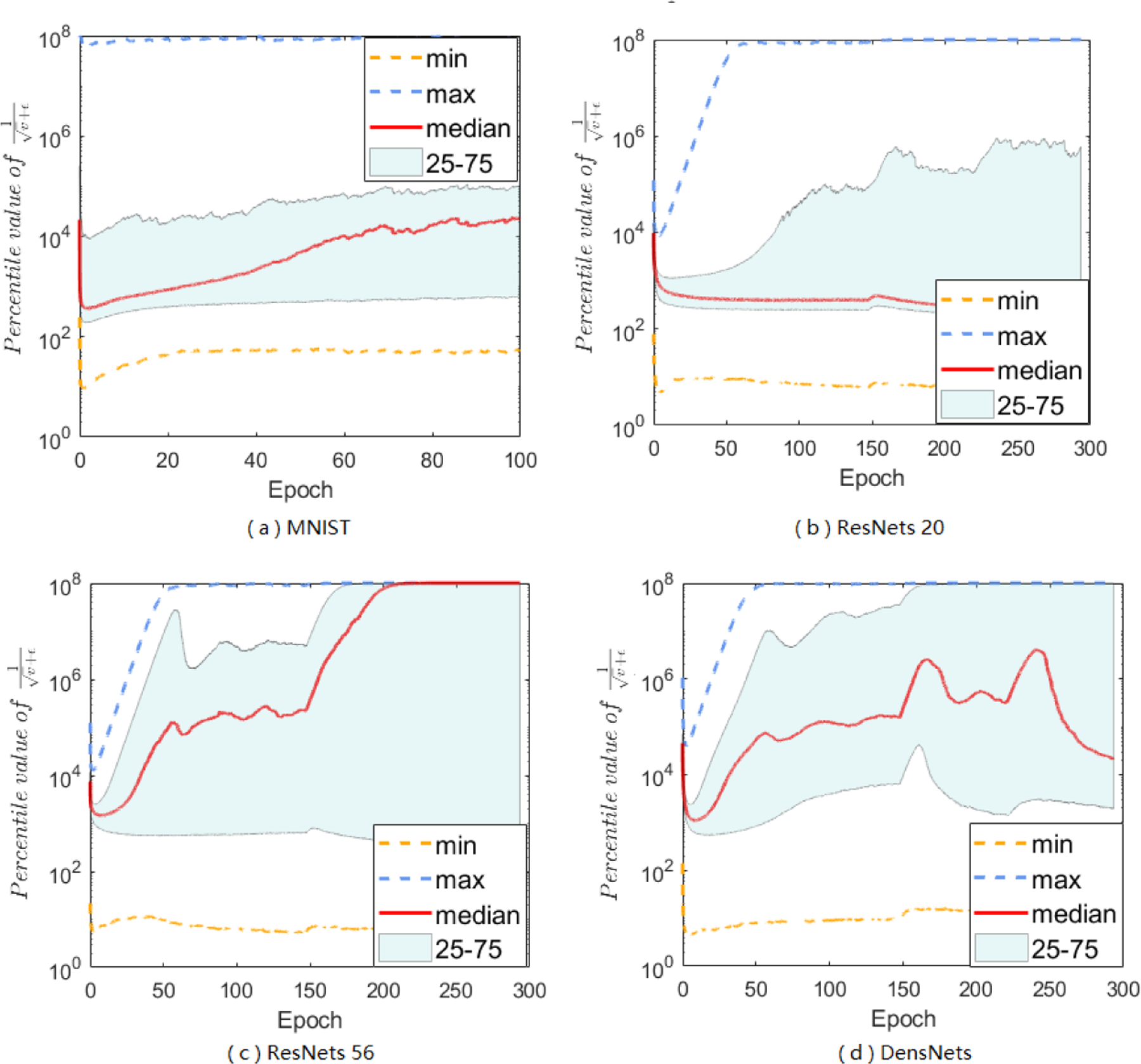
Range of the A-LR in Adam over iterations in four settings: (a) CNN on MNIST, (b) ResNet20 on CIFAR-10, (d) ResNet56 on CIFAR-10, (d) DenseNets on CIFAR-10. We plot the min, max, median, and the 25 and 75 percentiles of the A-LR across dimensions (the elements in $\frac{1}{\sqrt{v_t}+ϵ}$)

This anisotropic scale of A-LR across dimensions makes it difficult to determine the B-LR, η. On the one hand, η should be set small enough so that the $\text{LR}\frac{\eta }{\sqrt{v_t}+ϵ}$ is appropriate, or otherwise some coordinates will have very large updates because the corresponding A-LR’s are big, likely resulting in performance oscillation [21]. This may be due to that exponential moving average of past gradients is different, hence the speed of m_t diminishing to zero is different from the speed of $\sqrt{v_t}$ diminishing to zero. Besides, noise generated in stochastic algorithms has nonnegligible influence to the learning process. On the other hand, very small η may harm the later stage of the learning process since the small magnitude of m_t multiplying with a small step size (at some coordinates) will be too small to escape sharp local minimal, which has been shown to lead to poor generalization [22, 23, 24]. Further, in many deep learning tasks, stage-wise policies are often taken to decay the LR after several epochs, thus making the LR even smaller. To address the dilemma, it is essential to control the A-LR, especially when stochastic gradients get close to 0.

By analyzing previous modified AGMs that aim to close the generalization gap, we find that all these works can be summarized into one technique: constraining the A-LR, $1/\left(\sqrt{v_t}+ϵ\right)$, to a reasonable range. Based on the observation of anisotropic A-LR, we propose a more effective way to calibrate the A-LR according to an activation function rather than hard-thresholding the A-LR at all coordinates, empirically improve generalization performance with theoretical guarantees of optimization.

3.2. Sensitive to є.

As a hyper-parameter in AGMs, ϵ is originally introduced to avoid the zero denominator issue when v_t goes to 0, and has never been studied in the convergence analysis of AGMs. However, it has been empirically observed that AGMs can be sensitive to the choice of є in [17, 14]. As shown in Figure 1, a smaller є = 10⁻⁸ leads to a wide span of the A-LR across the different dimensions, whereas a bigger є = 10⁻³ as used in Yogi, reduces the span. To better learn the effect caused by sensitive є, we conduct experiments in multiple datasets and results are shown in Table 1 and 2. The setting of є is the main force causing anisotropy, unsatisfied, there has no theoretical result explains the effect of є on AGMs. Inspired by our observation, we believe that the current convergence analysis for Adam is not complete if omitting є.

Table 1:

Test Accuracy(%) of Adam for different є.

є	ResNets 20	ResNets 56	DenseNets	ResNet 18	VGG
10−1	92.51 ± 0.13	94.29 ± 0.10	94.78 ± 0.19	77.21 ± 0.26	76.05 ± 0.27
10−2	92.88 ± 0.21	94.15 ± 0.17	94.35 ± 0.10	76.64 ± 0.24	75.69 ± 0.16
10−4	92.03 ± 0.21	93.62 ± 0.18	94.15 ± 0.12	76.19 ± 0.20	74.45 ± 0.19
10−6	92.99 ± 0.22	93.56 ± 0.15	94.24 ± 0.24	76.09 ± 0.20	74.20 ± 0.33
10−8	91.68 ± 0.12	92.82 ± 0.09	93.32 ± 0.06	76.14 ± 0.24	74.18 ± 0.15

Table 2:

Test Accuracy(%) of AMSGrad for different є.

є	ResNets 20	ResNets 56	DenseNets	ResNet 18	VGG
10−1	92.80 ± 0.22	94.12 ± 0.07	94.92 ± 0.10	77.26 ± 0.30	75.84 ± 0.16
10−2	92.89 ± 0.07	94.20 ± 0.18	94.43 ± 0.22	76.23 ± 0.26	75.37 ± 0.18
10−4	91.85 ± 0.10	93.50 ± 0.14	94.02 ± 0.18	76.30 ± 0.31	74.44 ± 0.16
10−6	91.98 ± 0.23	93.54 ± 0.16	94.17 ± 0.10	76.14 ± 0.16	74.17 ± 0.28
10−8	91.70 ± 0.12	93.10 ± 0.11	93.71 ± 0.05	76.32 ± 0.11	74.26 ± 0.18

Most of the existing convergence analysis follows the line in [12] to first project the sequence of the iterates into a minimization problem as $x_{t+1}=x_t-\frac{\eta }{\sqrt{v_t}}{m}_t={\min }_x‖v_t^{1/4}\left(x-\left(x_t-\frac{\eta }{\sqrt{v_t}}{m}_t\right)\right)‖$, and then examine if $‖v_t^{1/4}\left(x_{t+1}-x^{\ast }\right)‖$ decreases over iterations. Hence, є is not discussed in this line of proof because it is not included in the step size. In our later convergence analysis section, we introduce an important lemma, bounded A-LR, and by using the bounds of the A-LR (specifically, the lower bound µ₁ and upper bound µ₂ both containing є for Adam), we give a new general framework of prove (details in Appendix) to show the convergence rate for reaching an x that satisfies $E\left[{‖\nabla f\left(x_t\right)‖}^2\right]\le \delta$ in the nonconvex setting. Then, we also derive the optimality gap from the stationary point in the convex and P-L settings (strongly convex).

Theorem 3.1. [Nonconvex] Suppose f(x) is a nonconvex function that satisfies Assumption 1. Let ${\eta }_t=\eta =O\left(\frac{1}{\sqrt{T}}\right)$, Adam has

$$\underset{t=1,\dots ,T}{\min }E\left[{‖\nabla f\left(x_t\right)‖}^2\right]\le O\left(\frac{1}{{ϵ}^2\sqrt{T}}+\frac{d}{ϵT}+\frac{d}{{ϵ}^{2}T\sqrt{T}}\right).$$

Theorem 3.2. [Non-strongly Convex] Suppose f(x) is a convex function that satisfies Assumption 1. Assume that $\forall t$, $E\left[‖x_t-x^{\ast }‖\le D\right.$, for any m ≠ n, $E\left[‖x_m-x_n‖\right]\le D_{\infty }$, let ${\eta }_t=\eta =O\left(\frac{1}{\sqrt{T}}\right)$, Adam has convergence rate $f\left({\overline{x}}_t\right)-f^{\ast }\le O\left(\frac{d}{{ϵ}^2\sqrt{T}}\right)$, where ${\overline{x}}_t=\frac{1}{T}{\sum }_{t=1}^T{x}_t$.

Theorem 3.3. [P-L Condition] Suppose f(x) has P-L condition (with parameter λ) holds under convex case, satisfying Assumption 1. Let ${\eta }_t=\eta =O\left(\frac{1}{T^2}\right)$, Adam has the convergence rate: $E\left[f\left(x_{T+1}\right)-f^{\ast }\right]\le {\left(1-\frac{2\lambda {\mu }_1}{T^2}\right)}^{T}E\left[f\left(x_1\right)-f^{\ast }\right]+O\left(\frac{1}{T}\right)$,

The P-L condition is weaker than strongly convex, and for the strongly convex case, we also have:

Corollary 3.3.1. [Strongly Convex] Suppose f(x) is µ-strongly convex function that satisfies Assumption 1. Let ${\eta }_t=\eta =O\left(\frac{1}{T^2}\right)$, Adam has the convergence rate: $E\left[f\left(x_{T+1}\right)-f^{\ast }\right]\le {\left(1-\frac{2\mu {\mu }_1}{T^2}\right)}^{T}E\left[f\left(x_1\right)-f^{\ast }\right]+O\left(\frac{1}{T}\right)$

This is the first time to theoretically include є into analysis. As expected, the convergence rate of Adam is highly related with є. A bigger є will enjoy a better convergence rate since є will dominate the A-LR and behaves like SMomentum; A smaller є will preserve stronger “adaptivity”, we need to find a better way to control є.

4. The Proposed Algorithms

We propose to use activation functions to calibrate AGMs, and specifically focus on using softplus funciton on top of Adam and AMSGrad methods.

4.1. Activation Functions Help

Activation functions (such as sigmoid, ELU, tanh) transfer inputs to outputs are widely used in deep learning area. As a well-studied activation function, $softplus\left(x\right)=\frac{1}{\beta }\log \left(1+e^{\beta x}\right)$ is known to keep large values unchanged (behaved like function y = x) while smoothing out small values (see Figure 2 (a)). The target magnitude to be smoothed out can be adjusted by a hyper-parameter $\beta \in ℝ$. In our new algorithms, we introduce $softplus\left(\sqrt{v_t}\right)=\frac{1}{\beta }\log \left(1+e^{\beta \cdot \sqrt{v_t}}\right)$ to smoothly calibrate the A-LR. This calibration brings the following benefits: (1) constraining extreme large-valued A-LR in some coordinates (corresponding to the small-values in v_t) while keeping others untouched with appropriate β. For the undesirable large values in the A-LR, the softplus function condenses them smoothly instead of hard thresholding. For other coordinates, the A-LR largely remains unchanged; (2) removing the sensitive parameter є because the softplus function can be lower-bounded by a nonzero number when used on non-negative variables, $softplus\left(\cdot \right)\ge \frac{1}{\beta }\log 2$.

Figure 2:

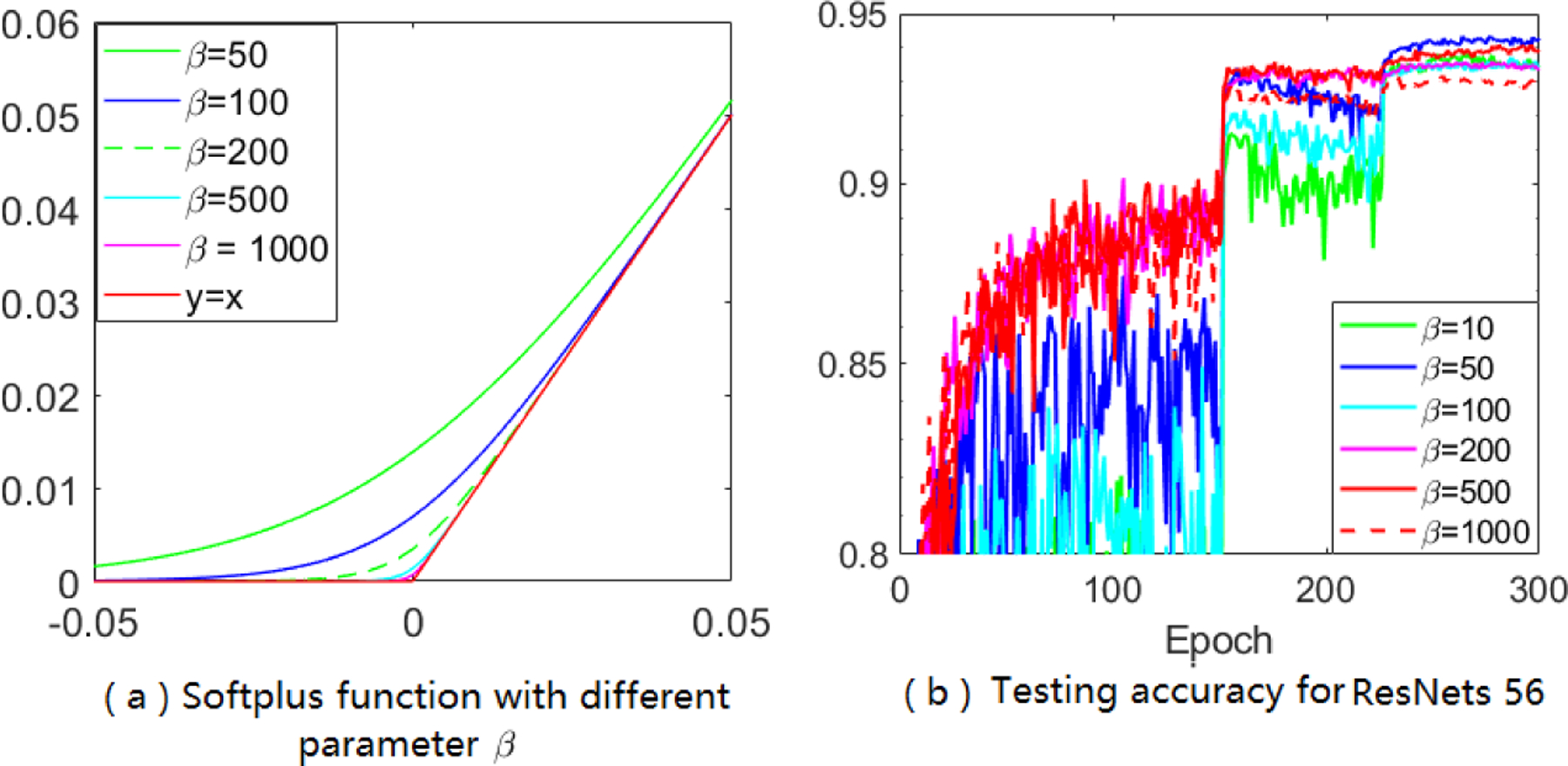
Behavior of the softplus function, and the test performance of our Sadam algorithm.

After calibrating $\sqrt{v_t}$ with a softplus function, the anisotropic A-LR becomes much more regulated (see Figure 3 and Appendix), and we clearly observe improved test accuracy (Figure 2 (b) and more figures in Appendix). We name this method “Sadam” to represent the calibrated Adam with softplus function, here we recommend using softplus function but it is not limited to that, and the later theoretical analysis can be easily extended to other activation functions. More empirical evaluations have shown that the proposed methods significantly improve the generalization performance of Adam and AMSGrad.

Figure 3:

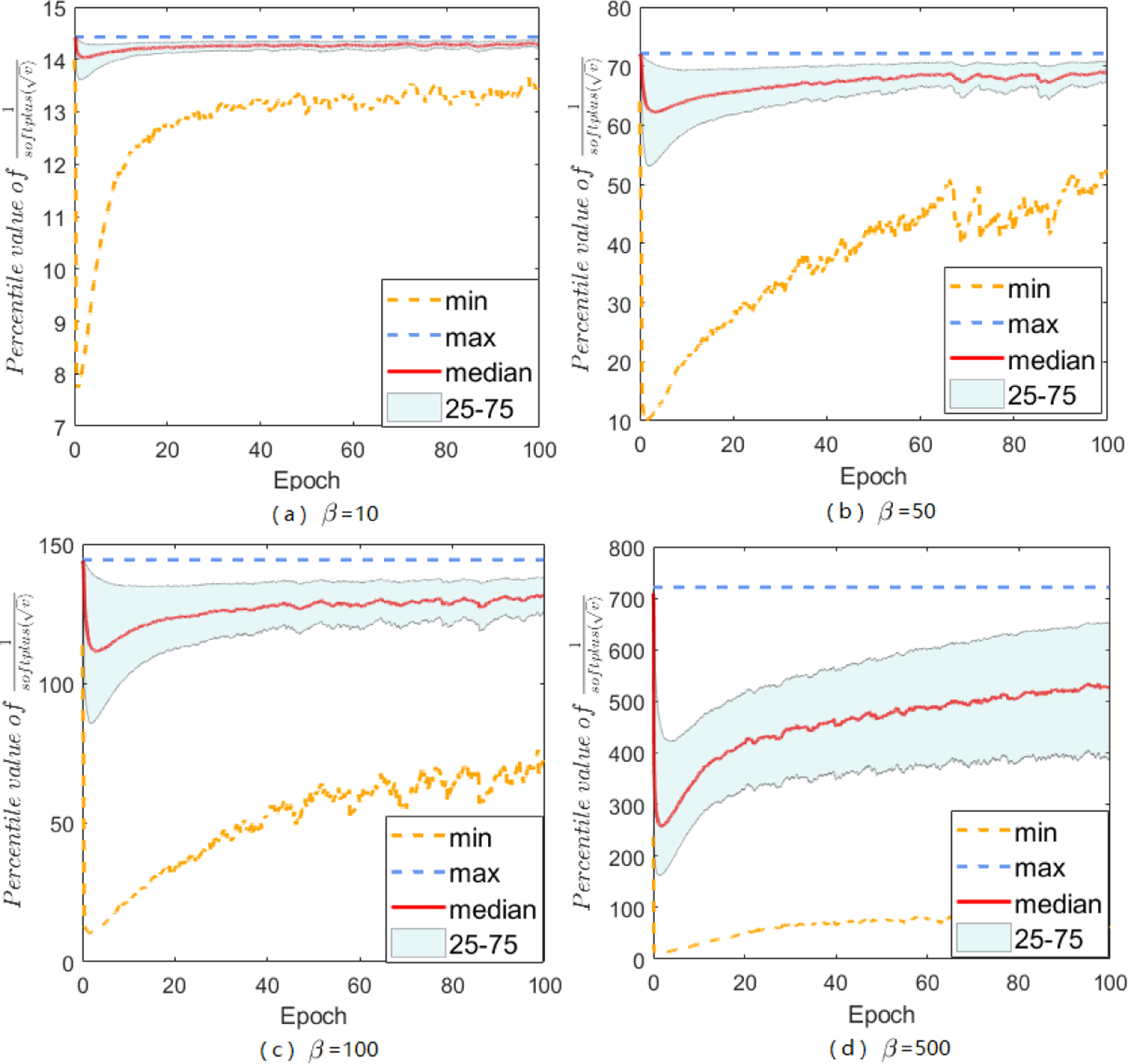
Behavior of the A-LR in the Sadam method with different choices of β (CNN on the MNIST data).

4.2. Calibrated AGMs

With activation function, we develop two new variants of AGMs: Sadam and SAMSGrad (Algorithms 1 and 2), which are developed based on Adam and AMSGrad respectively.

$$\overline{\underset{¯}{\begin{array}{l}\mathbf{\text{Algorithm\hspace{0.33em}}}\mathbf{1}\text{\hspace{0.33em}SADAM}\\ \overline{\begin{array}{l}\mathbf{\text{\hspace{1em}Input}}:x_1\in {ℝ}^d,\text{\hspace{0.33em}\hspace{0.33em}learning\hspace{0.33em}\hspace{0.33em}rate}\\ {\left\{{\eta }_t\right\}}_{t=1}^T,\text{\hspace{0.33em}\hspace{0.33em}parameters\hspace{0.33em}\hspace{0.17em}}0\le {\beta }_1,{\beta }_2<1,\\ \beta .\\ \mathbf{\text{\hspace{1em}Initialize\hspace{0.33em}}}{m}_0=0,v_0=0\\ \mathbf{\text{\hspace{1em}for\hspace{0.33em}}}t=1\text{\hspace{0.33em}to\hspace{0.33em}}T\mathbf{\text{\hspace{0.33em}do}}\\ \text{\hspace{1em}\hspace{1em}\hspace{0.17em}\hspace{0.17em}Compute stochastic gradient\hspace{0.33em}}{g}_t\\ m_t={\beta }_1{m}_{t-1}+\left(1-{\beta }_1\right)g_t\\ v_t={\beta }_2{v}_{t-1}+\left(1-{\beta }_2\right)g_t^2\\ \\ x_{t+1}=x_t-\frac{{\eta }_t}{softplus\left(\sqrt{v_t}\right)}\odot m_t\\ \mathbf{\text{\hspace{1em}end\hspace{0.33em}for}}\end{array}}\end{array}}}$$

$$\overline{\underset{¯}{\begin{array}{l}\mathbf{\text{Algorithm\hspace{0.33em}}}\mathbf{2}\text{\hspace{0.33em}SAMSGRAD}\\ \overline{\begin{array}{l}\mathbf{\text{\hspace{1em}Input}}:x_1\in {ℝ}^d,\text{\hspace{0.33em}\hspace{0.33em}learning\hspace{0.33em}\hspace{0.33em}rate}\\ {\left\{{\eta }_t\right\}}_{t=1}^T,\text{\hspace{0.33em}\hspace{0.33em}parameters\hspace{0.33em}\hspace{0.17em}}0\le {\beta }_1,{\beta }_2<1,\\ \beta .\\ \mathbf{\text{\hspace{1em}Initialize\hspace{0.33em}}}{m}_0=0,{\tilde{v}}_0=0\\ \mathbf{\text{\hspace{1em}for\hspace{0.33em}}}t=1\text{\hspace{0.33em}to\hspace{0.33em}}T\mathbf{\text{\hspace{0.33em}do}}\\ \text{\hspace{1em}\hspace{1em}\hspace{0.17em}\hspace{0.17em}Compute stochastic gradient\hspace{0.33em}}{g}_t\\ m_t={\beta }_1{m}_{t-1}+\left(1-{\beta }_1\right)g_t\\ {\tilde{v}}_t={\beta }_2{\tilde{v}}_{t-1}+\left(1-{\beta }_2\right)g_t^2\\ v_t=max\left\{v_{t-1},{\tilde{v}}_t\right\}\\ x_{t+1}=x_t-\frac{{\eta }_t}{softplus\left(\sqrt{v_t}\right)}\odot m_t\\ \mathbf{\text{\hspace{1em}end\hspace{0.33em}for}}\end{array}}\end{array}}}$$

The key step lies in the way to design the adaptive functions, instead of using the generalized square root function only, we apply softplus(·) on top of the square root of the second-order momentum, which serves to regulate A-LR’s anisotropic behavior and replace the tolerance parameter є by the hyper-parameter β used in the softplus function.

In our algorithms, the hyper-parameters are recommended as β₁ = 0.9, β₂ = 0.999. For clarity, we omit the bias correction step proposed in the original Adam. However, our arguments and theoretical analysis are applicable to the bias correction version as well [6, 25, 14]. Using the softplus function, we introduce a new hyper-parameter β, which performs as a controller to smooth out anisotropic A-LR, and connect the Adam and S-Momentum methods automatically. When β is set to be small, Sadam and SAMSGrad perform similarly to S-Momentum; when β is set to be big, $softplus\left(\sqrt{v_t}\right)=\frac{1}{\beta }\log \left(1+e^{\beta \cdot \sqrt{v_t}}\right)\approx \frac{1}{\beta }\log \left(e^{\beta \cdot \sqrt{v_t}}\right)=\sqrt{v_t}$, and the updating formula becomes $x_{t+1}=x_t-\frac{{\eta }_t}{\sqrt{v_t}}\odot m_t$, which is degenerated into the original AGMs. The hyper-parameter β can be well tuned to achieve the best performance for different datasets and tasks. Based on our empirical observations, we recommend to use β = 50.

As a calibration method, the softplus function has better adaptive behavior than simply setting. More precisely, when є is large or β is small, Adam and AMSGrad amount to S-Momentum, but when є is small as commonly suggested 10⁻⁸ or β is taken large, the two methods are different because comparing Figure 1 and 3 yields that Sadam has more regulated A-LR distribution. The proposed calibration scheme regulates the massive range of A-LR back down to a moderate scale. The median of A-LR in different dimensions is now well positioned to the middle of the 25–75 percentile zone. Our approach opens up a new direction to examine other activation functions (not limited to the softplus function) to calibrate the A-LR.

The proposed Sadam and SAMSGrad can be treated as members of a class of AGMs that use the softplus (or another suitable activation) function to better adapt the step size. It can be readily combined with any other AGM, e.g., Rmsrop, Yogi, and PAdam. These methods may easily go back to the original ones by choosing a big β.

5. Convergence Analysis

We first demonstrate an important lemma to highlight that every coordinate in the A-LR is both upper and lower bounded at all iterations, which is consistent with empirical observations (Figure 1), and forms the foundation of our proof.

Lemma 5.1. [Bounded A-LR] With Assumption 1, for any t ≥ 1, j ∈ [1,d], β₂ ∈ [0,1], and in Adam, β in Sadam, anisotropic A-LR is bounded in AGMs, Adam has (µ₁,µ₂)-bounded A-LR:

$${\mu }_1\le \frac{1}{\sqrt{v_{t,j}}+ϵ}\le {\mu }_2,$$

Sadam has (µ₃,µ₄)-bounded A-LR:

$${\mu }_3\le \frac{1}{softplus\left(\sqrt{v_{t,j}}\right)}\le {\mu }_4,$$

where 0 < µ₁ ≤ µ₂, and 0 < µ₃ ≤ µ₄

Remark 5.2. Besides the square root function and softplus function, the A-LR calibrated by any positive monotonically increasing function can be bounded. All of the bounds can be shown to be related to є or β (see Appendix). Bounded A-LR is an essential foundation in our analysis, we provide a different way of proof from previous works, and the proof procedure can be easily extended to other gradient methods as long as bounded LR is satisfied.

Remark 5.3. These bounds can be applied to all AGMs, including Adagrad. In fact, the lower bounds actually are not the same in Adam and Adagrad, because Adam will have smaller $\sqrt{v_{t,j}}$ due to moment decay parameter β₂. To achieve a unified result, we use the same relaxation to derive the fixed lower bound µ₁.

We now describe our main results of Sadam (and SAMSGrad) in the nonconvex case, we clearly show that similar to Theorem 3.1, the convergence rate of Sadam is related to the bounds of the A-LR. Our methods have improved the convergence rate of Adam when comparing self-contained parameters є and β.

Theorem 5.4. [Nonconvex] Suppose f(x) is a nonconvex function that satisfies Assumption 1. Let ${\eta }_t=\eta =O\left(\frac{1}{\sqrt{T}}\right)$, Sadam method has

$$\underset{t=1,\dots ,T}{\min }E\left[{‖\nabla f\left(x_t\right)‖}^2\right]\le O\left(\frac{{\beta }^2}{\sqrt{T}}+\frac{d\beta }{T}+\frac{d{\beta }^2}{T\sqrt{T}}\right).$$

Remark 5.5. Compared with the rate in Theorem 3.1, the convergence rate of Sadam relies on β, which can be a much smaller number (β = 50 as recommended) than $\frac{1}{ϵ}$ (commonly є = 10⁻⁸ in AGMs), showing that our methods have a better convergence rate than Adam. When β is huge, Sadam’s rate is comparable to the classic Adam. When β is small, the convergence rate will be $O\left(\frac{1}{\sqrt{T}}\right)$ which recovers that of SGD [1].

Corollary 5.5.1. Treat є or β as a constant, then the Adam, Sadam (and SAMSGrad) methods with fixed L,σ,G,β₁, and $\eta =O\left(\frac{1}{\sqrt{T}}\right)$, have complexity of $O\left(\frac{1}{\sqrt{T}}\right)$, and thus call for $O\left(\frac{1}{{\delta }^2}\right)$ iterations to achieve δ-accurate solutions.

Theorem 5.6. [Non-strongly Convex] Suppose f(x) is a convex function that satisfies Assumption 1. Assume that $E\left[‖x_t-x^{\ast }‖\right]\le D,\forall t$, and $E\left[‖x_m-x_n‖\right]\le D_{\infty }$, $\forall m\ne n$, let ${\eta }_t=\eta =O\left(\frac{1}{\sqrt{T}}\right)$, Sadam has $f\left({\overline{x}}_t\right)-f^{\ast }\le O\left(\frac{1}{\sqrt{T}}\right)$, where ${\overline{x}}_t=\frac{1}{T}{\sum }_{t=1}^T{x}_t$.

The accurate convergence rate will be $O\left(\frac{d}{{ϵ}^2\sqrt{T}}\right)$ for Adam and $O\left(\frac{d{\beta }^2}{\sqrt{T}}\right)$ for Sadam with fixed L, σ, G, β₁, D, D_∞. Some works may specify additional sparsity assumptions on stochastic gradients, and in other words, require that ${\sum }_{t=1}^T{\sum }_{j=1}^d‖g_{t,j}‖\ll \sqrt{dT}$ [5, 12, 15, 19] to reduce the order from d to $\sqrt{d}$. Some works may use the element-wise bounds σ_j or G_j, and apply ${\sum }_{j=1}^d{\sigma }_j=\sigma$, and ${\sum }_{j=1}^d{G}_j=G$ to hide d. In our work, we do not assume sparsity, so we use σ and G throughout the proof. Otherwise, those techniques can also be used to hide d from our convergence rate.

Corollary 5.6.1. If є or β is treated as constants, then Adam, Sadam (and SAMSGrad) methods with fixed L,σ,G,β₁, and $\eta =O\left(\frac{1}{\sqrt{T}}\right)$ in the convex case will call for $O\left(\frac{1}{{\delta }^2}\right)$ iterations to achieve δ-accurate solutions.

Theorem 5.7. [P-L Condition] Suppose f(x) satisfies the P-L condition (with parameter λ) and Assumption 1 in the convex case. Let ${\eta }_t=\eta =O\left(\frac{1}{T^2}\right)$, Sadam has:

$$E\left[f\left(x_{T+1}\right)-f^{\ast }\right]\le {\left(1-\frac{2\lambda {\mu }_3}{T^2}\right)}^{T}E\left[f\left(x_1\right)-f^{\ast }\right]+O\left(\frac{1}{T}\right).$$

Corollary 5.7.1. [Strongly Convex] Suppose f(x) is µ-strongly convex function that satisfies Assumption 1. Let ${\eta }_t=\eta =O\left(\frac{1}{T^2}\right)$, Sadam has the convergence rate:

$$E\left[f\left(x_{T+1}\right)-f^{\ast }\right]\le {\left(1-\frac{2\mu {\mu }_3}{T^2}\right)}^{T}E\left[f\left(x_1\right)-f^{\ast }\right]+O\left(\frac{1}{T}\right).$$

In summary, our methods share the same convergence rate as Adam, and enjoy even better convergence speed if comparing the common values chosen for the parameters є and β. Our convergence rate recovers that of SGD and S-Momentum in terms of T for a small β.

6. Experiments

We compare Sadam and SAMSGrad against several state-of-the-art optimizers including S-Momentum, Adam, AMSGrad, Yogi, PAdam, PAMSGrad, Adabound, and Amsbound. More results and architecture details are in Appendix.

Experimental Setup.

We use three datasets for image classifications: MNIST, CIFAR-10 and CIFAR-100 and two datasets for LSTM language models: Penn Treebank dataset (PTB) and the WikiText-2 (WT2) dataset. The MNIST dataset is tested on a CNN with 5 hidden layers. The CIFAR-10 dataset is tested on Residual Neural Network with 20 layers (ResNets 20) and 56 layers (ResNets 56) [9], and DenseNets with 40 layers [11]. The CIFAR-100 dataset is tested on VGGNet [26] and Residual Neural Network with 18 layers (ResNets 18) [9]. The Penn Treebank dataset (PTB) and the WikiText-2 (WT2) dataset are tested on 3-layer LSTM models [27].

We train CNN on the MNIST data for 100 epochs, ResNets/DenseNets on CIFAR-10 for 300 epochs, with a weight decay factor of 5 × 10⁻⁴ and a batch size of 128, VGGNet/ResNets on CIFAR-100 for 300 epochs, with a weight decay factor of 0.025 and a batch size of 128 and LSTM language models on 200 epochs. For the CIFAR tasks, we use a fixed multi-stage LR decaying scheme: the B-LR decays by 0.1 at the 150-th epoch and 225-th epoch, which is a popular decaying scheme used in many works [28, 18]. For the language tasks, we use a fixed multi-stage LR decaying scheme: the B-LR decays by 0.1 at the 100-th epoch and 150-th epoch. All algorithms perform grid search for hyperparameters to choose from {10,1,0.1,0.01,0.001,0.0001} for B-LR, {0.9,0.99} for β₁ and {0.99,0.999} for β₂. For algorithm-specific hyper-parameters, they are tuned around the recommended values, such as $p\in \left\{\frac{1}{8},\frac{1}{16}\right\}$ in PAdam and PAMSGrad. For our algorithms, β is selected from {10,50,100} in Sadam and SAMSGrad, though we do observe fine-tuning β can achieve better test accuracy most of time. All experiments on CIFAR tasks are repeated for 6 times to obtain the mean and standard deviation for each algorithm.

Image Classification Tasks.

As a sanity check, experiment on MNIST has been done and its results are in Figure 4, which shows the learning curve for all baseline algorithms and our algorithms on both training and test datasets. As expected, all methods can reach the zero loss quickly, while for test accuracy, our SAMSGrad shows increase in test accuracy and outperforms competitors within 50 epochs.

Figure 4:

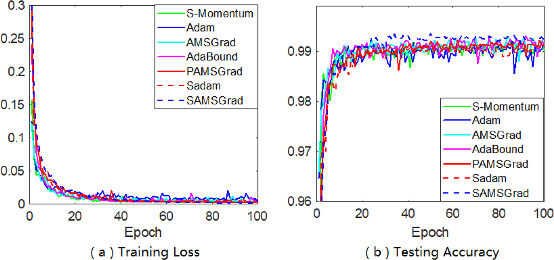
Training loss and test accuracy on MNIST.

Using the PyTorch framework, we first run the ResNets 20 model on CIFAR10 and results are shown in Table 3. The original Adam and AMSGrad have lower test accuracy in comparison with S-Momentum, leaving a clear generalization gap exactly same as what is previously reported. For our methods, Sadam and SAMSGrad clearly close the gap, and Sadam achieves the best test accuracy among competitors. We further test all methods with CIFAR10 on ResNets 56 with greater network depth, and the overall performance of each algorithm has been improved. For the experiments with DenseNets, we use a DenseNet with 40 layers and a growth rate k = 12 without bottleneck, channel reduction, or dropout. The results are reported in the last column of Table 3, SAMSGrad still achieves the best test performance, and the proposed two methods largely improve the performance of Adam and AMSGrad and close the gap with S-Momentum.

Table 3:

Test Accuracy(%) of CIFAR-10 for ResNets 20, ResNets 56 and DenseNets.

Method	B-LR	є	β	ResNets 20	ResNets 56	DenseNets
S-Momentum [9, 11]	-	-	-	91.25	93.03	94.76
Adam [14]	10−3	10−3	-	92.56 ± 0.14	93.42 ± 0.16	93.35 ± 0.21
Yogi [14]	10−2	10−3	-	92.62 ± 0.17	93.90 ± 0.21	94.38 ± 0.26
S-Momentum	10−1	-	-	92.73 ± 0.05	94.11 ± 0.15	95.03 ± 0.15
Adam	10−3	10−8	-	91.68 ± 0.12	92.82 ± 0.09	93.32 ± 0.06
AMSGrad	10−3	10−8	-	91.7 ± 0.12	93.10 ± 0.11	93.71 ± 0.05
PAdam	10−1	10−8	-	92.7 ± 0.10	94.12 ± 0.12	95.06 ± 0.06
PAMSGrad	10−1	10−8	-	92.74 ± 0.12	94.18 ± 0.06	95.21 ± 0.10
AdaBound	10−2	10−8	-	91.59 ± 0.24	93.09 ± 0.14	94.16 ± 0.10
AmsBound	10−2	10−8	-	91.76 ± 0.16	93.08 ± 0.09	94.03 ± 0.11
Adam+	10−1	0.013	-	92.89 ± 0.13	92.24 ± 0.10	94.54 ± 0.13
AMSGrad+	10−1	0.013	-	92.95 ± 0.17	94.32 ± 0.10	94.58 ± 0.18
Sadam	10−2	-	50	93.01 ± 0.16	94.26 ± 0.10	95.19 ± 0.18
SAMSGrad	10−2	-	50	92.88 ±0.10	94.32 ± 0.18	95.31 ± 0.15

Furthermore, two popular CNN architectures: VGGNet [26] and ResNets18 [9] are tested on CIFAR-100 dataset to compare different algorithms. Results can be found in Figure 5 and repeated results are in Appendix. Our proposed methods again perform slightly better than S-Momentum in terms of test accuracy.

Figure 5:

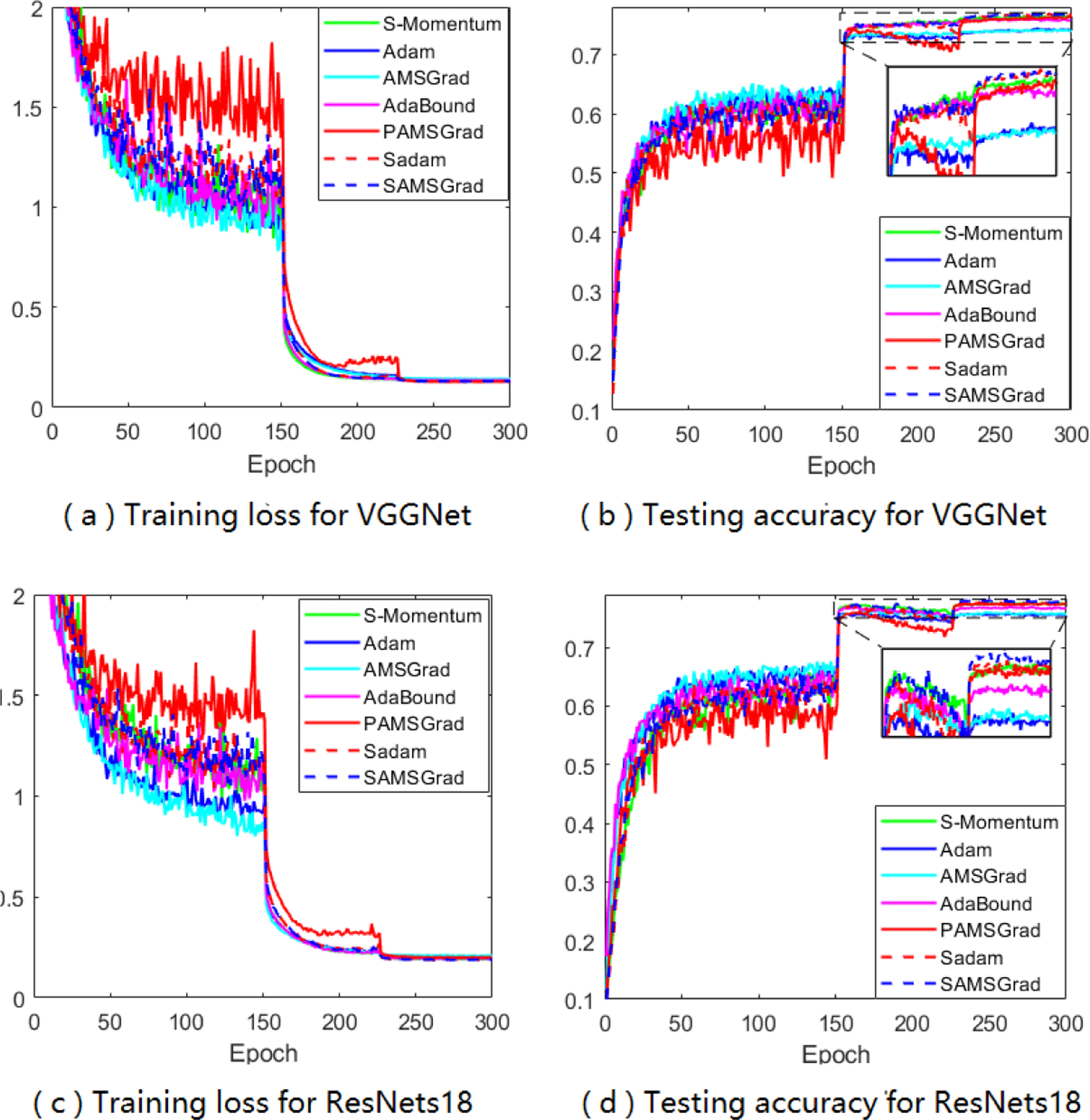
Training loss and test accuracy of two CNN architectures on CIFAR-100.

LSTM Language Models.

Observing the significant improvements in deep neural networks for image classification tasks, we further conduct experiments on the language models with LSTM. For comparing the efficiency of our proposed methods, two LSTM models over the Penn Treebank dataset (PTB) [29] and the WikiText-2 (WT2) dataset [30] are tested. We present the single-model perplexity results for both our proposed methods and other competitive methods in Figure 6 and our methods achieve both fast convergence and best generalization performance.

Figure 6:

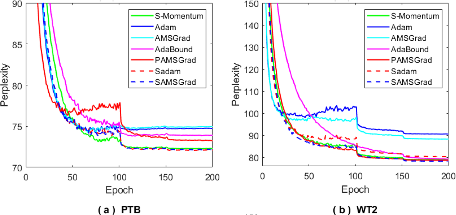
Perplexity curves on the test set on 3-layer LSTM models over PTB and WT2 datasets

In summary, our proposed methods show great efficacy on several standard benchmarks in both training and testing results, and outperform most optimizers in terms of generalization performance.

7. Conclusion

In this paper, we study adaptive gradient methods from a new perspective that is driven by the observation that the adaptive learning rates are anisotropic at each iteration. Inspired by this observation, we propose to calibrate the adaptive learning rates using an activation function, and in this work, we examine softplus function. We combine this calibration scheme with Adam and AMSGrad methods and empirical evaluations show obvious improvement on their generalization performance in multiple deep learning tasks. Using this calibration scheme, we replace the hyper-parameter є in the original methods by a new parameter β in the softplus function. A new mathematical model has been proposed to analyze the convergence of adaptive gradient methods. Our analysis shows that the convergence rate is related to є or β, which has not been previously revealed, and the dependence on є or β helps us justify the advantage of the proposed methods. In the future, the calibration scheme can be designed based on other suitable activation functions, and used in conjunction with any other adaptive gradient method to improve generalization performance.

Appendix

A.1. Architecture Used in Our Experiments

Here we mainly introduce the MNIST architecture with Pytorch used in our empirical study, ResNets and DenseNets are well-known architectures used in many works and we do not include details here.

layer	layer setting
F.relu(self.conv1(x))	self.conv1 = nn.Conv2d(1, 6, 5)
F.max pool2d(x, 2, 2)
F.relu(self.conv2(x))	self.conv2 = nn.Conv2d(6, 16, 5)
x.view(−1, 16*4)
F.relu(self.fc1(x))	self.fc1 = nn.Linear(16*4*4, 120)
x= F.relu(self.fc2(x))	self.fc2 = nn.Linear(120, 84)
x = self.fc3(x)	self.fc3 = nn.Linear(84, 10)
F.log softmax(x, dim=1)

B.2. More Empirical Results

In this section, we perform multiply experiments to study the property of anisotropic A-LR exsinting in AGMs and the performance of softplus function working on A-LR. We first show the A-LR range of popular Adam-type methods, then present how the parameter β in Sadam and SAMSGrad reduce the range of A-LR and improve both training and testing performance.

B.2.1. A-LR Range of AGMs

Besides the A-LR range of Adam method, which has shown in main paper, we further want to study more other Adam-type methods, and do experiments focus on AMSGrad, PAdam, and PAMSGrad on different tasks (Figure B.2.1, B.2.2, and B.2.3). AMSGrad also has extreme large-valued coordinates, and will encounter the “small learning rate dilemma” as well as Adam. With partial parameter p, the value range of A-LR can be largely narrow down, and the maximum range will be reduced around 10² with PAdam, and less than 10² with PAMSGrad. This reduced range, avoiding the “small learning rate dilemma”, may help us understand what “trick” works on Adam’s A-LR can indeed improve the generalization performance. Besides, the range of A-LR in Yogi, Adabound and Amsbound will be reduced or controlled by specific є or clip function, we don’t show more information here.

B.2.2. Parameter β Reduces the Range of A-LR

The main paper has discussed about softplus function, and mentions that it does help to constrain large-valued coordinates in A-LR while keep others untouched, here we give more empirical support. No matter how does β set, the modified A-LR will have a reduced range. By setting various β’s, we can find an appropriate β that performs the best for specific tasks on datasets. Besides the results of A-LR range of Sadam on MNIST with different choices of β, we also study Sadam and SAMSGrad on ResNets 20 and DenseNets.

Here we do grid search to choose appropriate β from {10,50,100,200,500,1000}. In summary, with softplus fuction, Sadam and SAMSGrad will narrow down the range of A-LR, make the A-LR vector more regular, avoiding ”small learning rate dilemma” and finally achieve better performance.

B.2.3. Parameter β Matters in Both Training and Testing

After studying existing Adam-type methods, and effect of different β in adjusting A-LR, we focus on the training and testing accuracy of our softplus framework, especially Sadam and SAMSGrad, with different choices of β.

Figure B.2.1:

A-LR range of AMSGrad (a), PAdam (b), and PAMSGrad (c) on MNIST.

Figure B.2.2:

A-LR range of AMSGrad (a), PAdam (b), and PAMSGrad (c) on ResNets 20.

Figure B.2.3:

A-LR range of AMSGrad (a), PAdam (b), and PAMSGrad (c) on DenseNets.

Figure B.2.4:

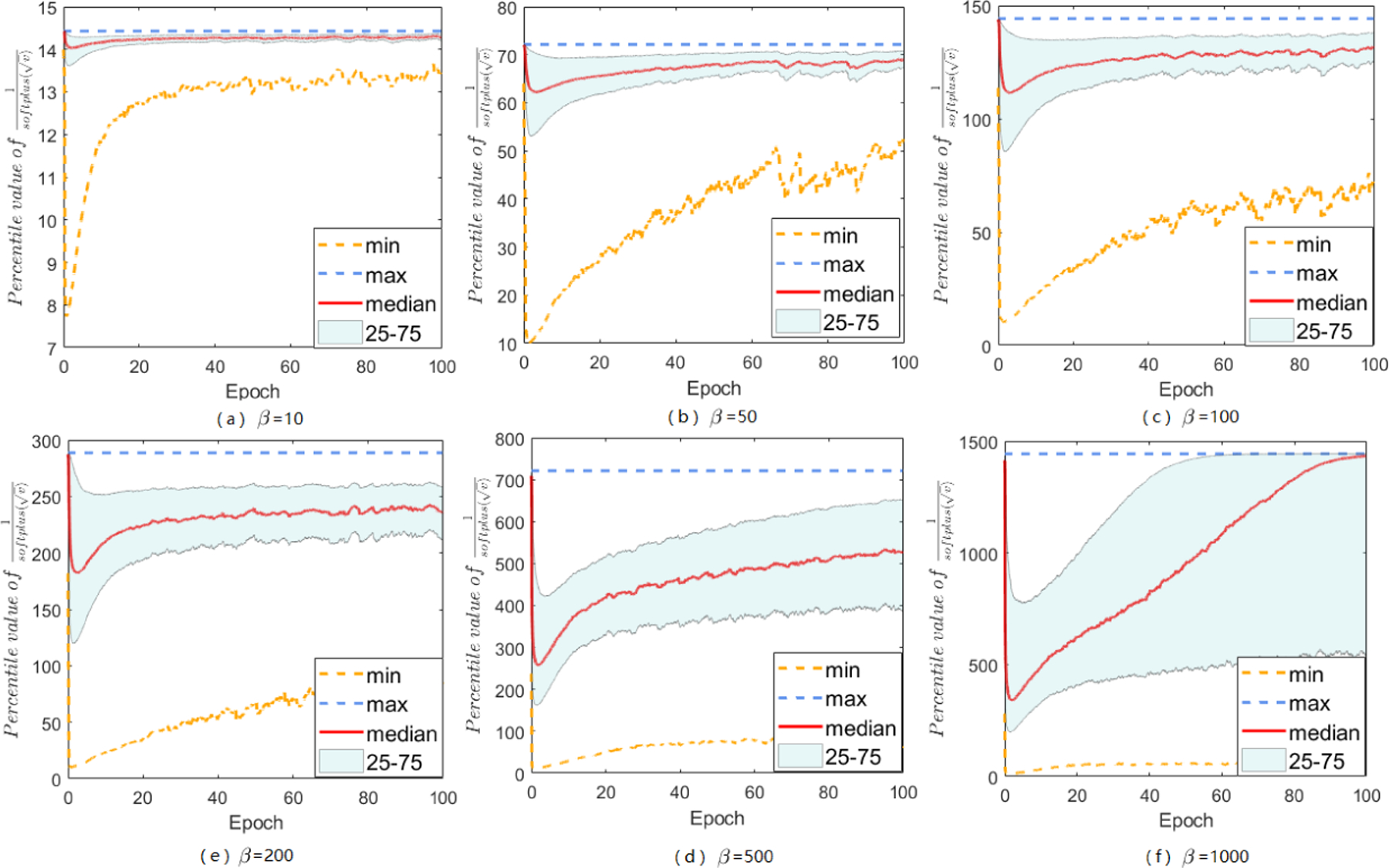
The range of A-LR: $1/softplus\left(\sqrt{v_t}\right)$ over iterations for different choices of β. The maximum ranges in all figures are compressed to a reasonable smaller value compared with 10⁸.

Figure B.2.5:

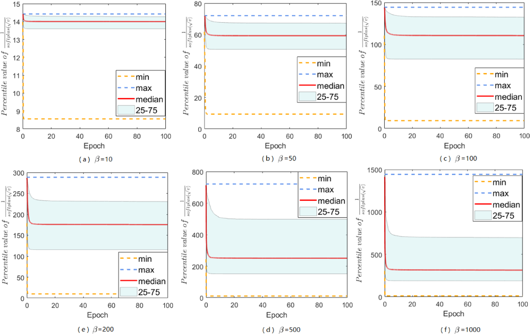
The range of A-LR: $1/softplus\left(\sqrt{v_t}\right)$, $v_t=max\left\{v_{t-1},{\tilde{v}}_t\right\}$ over iterations for SAMSGrad on MNIST with different choice of β. The maximum ranges in all figures are compressed to a reasonable smaller value compared with those of AMSGrad on MNIST

Figure B.2.6:

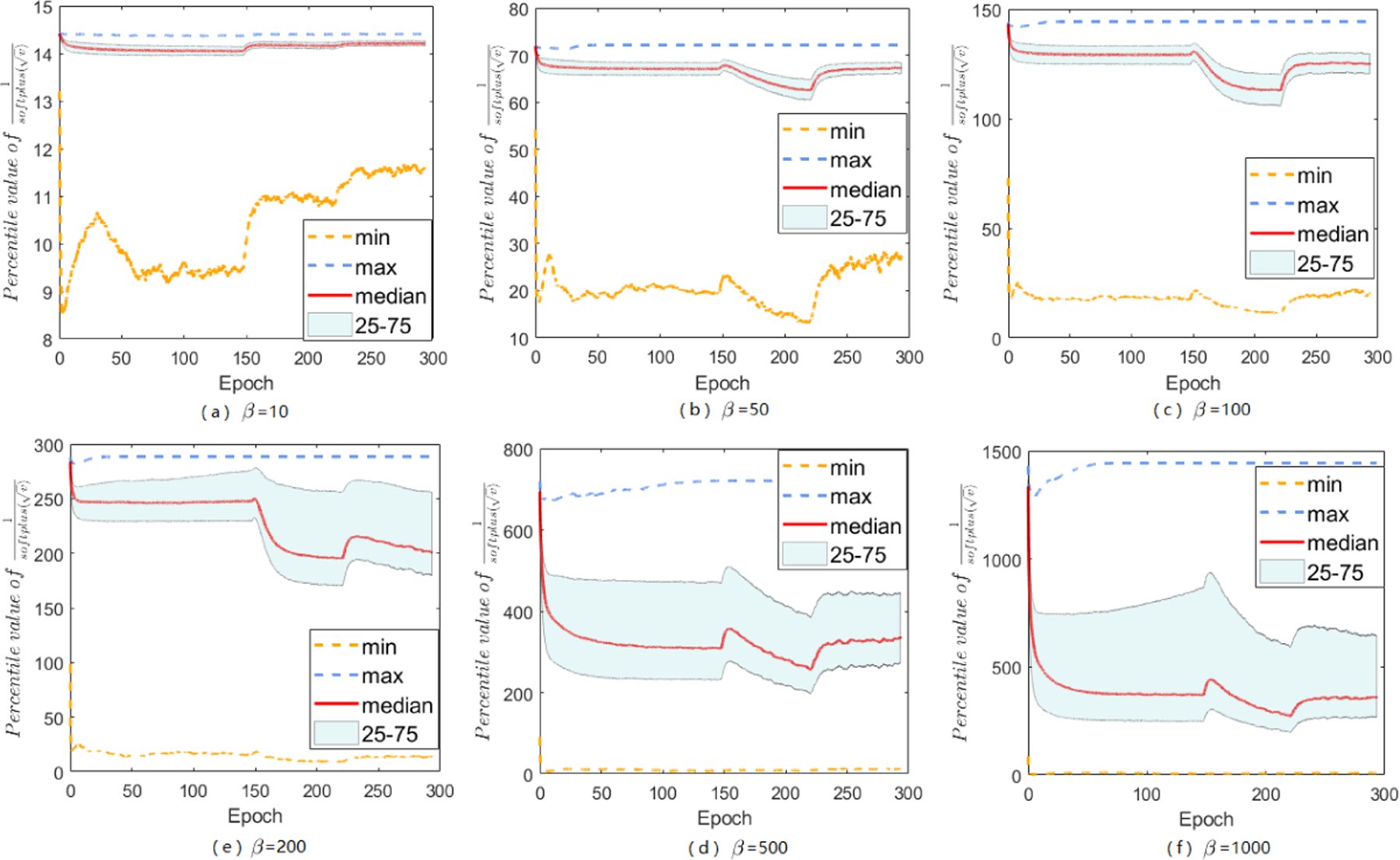
The range of A-LR: $1/softplus\left(\sqrt{v_t}\right)$ over iterations for Sadam on ResNets 20 with different choices of β.

Figure B.2.7:

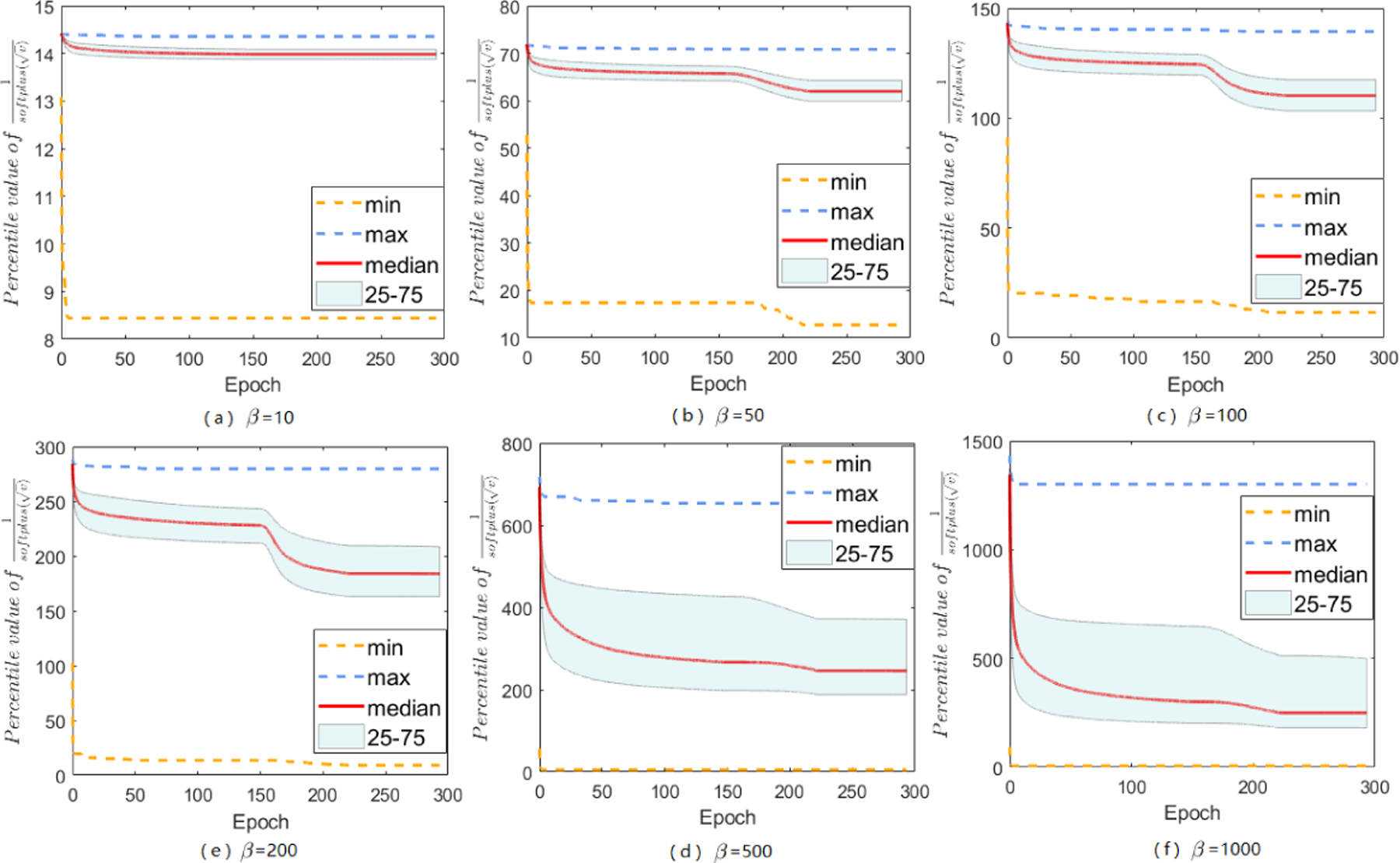
The range of A-LR: $1/softplus\left(\sqrt{v_t}\right)$, $v_t=max\left\{v_{t-1},{\tilde{v}}_t\right\}$ over iterations for SAMSGrad on ResNets 20 with different choices of β.

Figure B.2.8:

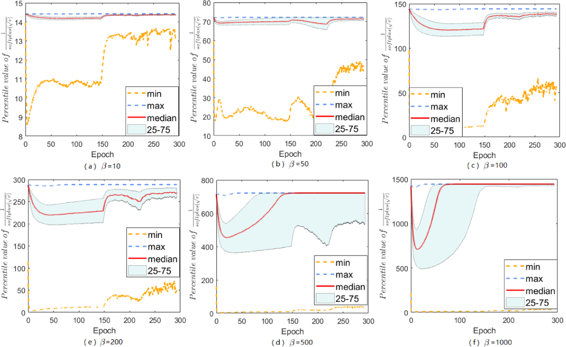
The range of A-LR: $1/softplus\left(\sqrt{v_t}\right)$ over iterations for Sadam on DenseNets with different choice of β.

Figure B.2.9:

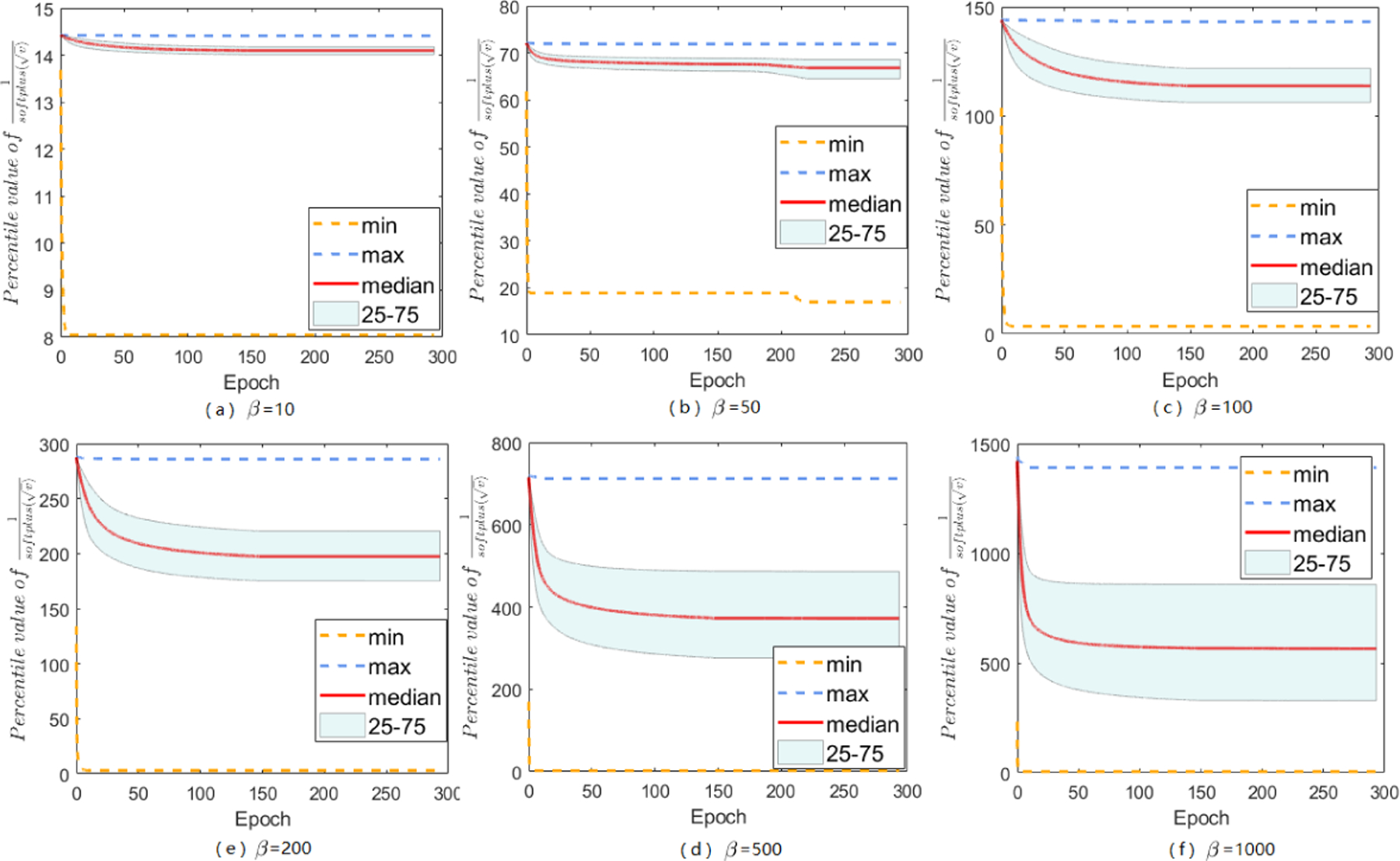
The range of A-LR: $1/softplus\left(\sqrt{v_t}\right)$, $v_t=max\left\{v_{t-1},{\tilde{v}}_t\right\}$ over iterations for SAMSGrad on DenseNets with different choices of β.

Figure B.2.10:

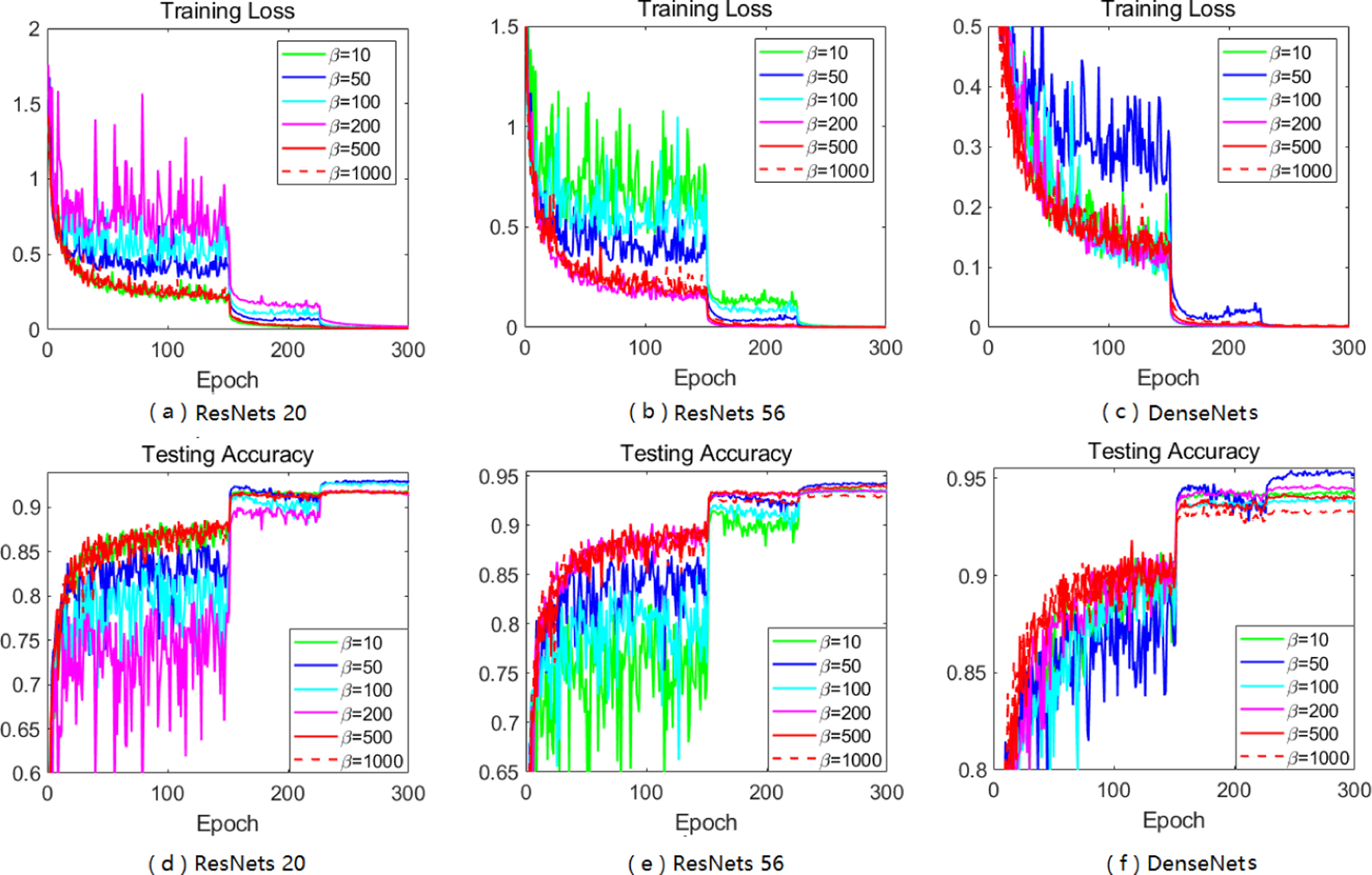
Performance of Sadam on CIFAR-10 with different choice of β.

Figure B.2.11:

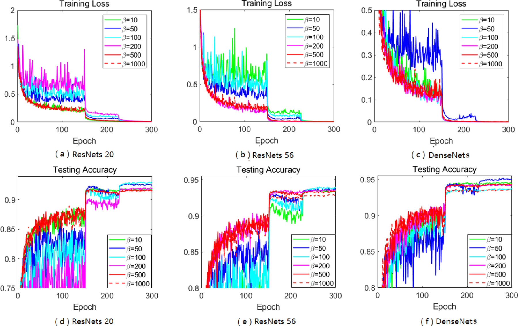
Performance of SAMSGrad on CIFAR-10 with different choice of β.

C.3. CIFAR100

Two popular CNN architectures are tested on CIFAR-100 dataset to compare different algorithms: VGGNet [26] and ResNets18 [9]. Besides the figures in main text, we have repeated experiments and show results as follows. Our proposed methods again perform slightly better than S-Momentum in terms of D.4. Theoretical Analysis Details

Table C.3.1:

Test Accuracy(%) of CIFAR100 for VGGNet.

Method	50th epoch	150th epoch	250th epoch	best perfomance
S-Momentum	59.09 ± 2.09	61.25 ± 1.51	76.14 ± 0.12	76.43 ± 0.15
Adam	60.21 ± 0.81	62.98 ± 0.10	73.81 ± 0.17	74.18 ± 0.15
AMSGrad	61.00 ± 1.17	63.27 ± 1.18	74.04 ± 0.16	74.26 ± 0.18
PAdam	53.62 ± 1.70	56.02 ± 0.86	75.85 ± 0.20	76.36 ± 0.16
PAMSGrad	52.49 ± 3.07	57.39 ± 1.40	75.82 ± 0.31	76.26 ± 0.30
AdaBound	60.27 ± 0.99	60.36 ± 1.71	75.86 ± 0.23	76.10 ± 0.22
AmsBound	59.88 ± 0.56	60.11 ± 1.92	75.74 ± 0.23	75.99 ± 0.20
Adam+	43.59 ± 2.71	44.46 ± 4.39	74.91 ± 0.36	75.58 ± 0.33
AMSGrad+	44.45 ± 2.83	45.61 ± 3.67	74.85 ± 0.08	75.56 ± 0.24
Sadam	58.59 ± 1.60	61.27 ± 1.67	76.35 ± 0.18	76.64 ± 0.18
SAMSgrad	59.16 ± 1.20	60.86 ± 0.39	76.27 ± 0.23	76.47 ± 0.26

Table C.3.2:

Test Accuracy(%) of CIFAR100 for ResNets18.

Method	50th epoch	150th epoch	250th epoch	best perfomance
S-Momentum	59.98 ± 1.31	63.32 ± 1.61	77.19 ± 0.36	77.50 ± 0.25
Adam	63.40 ± 1.42	66.18 ± 1.02	75.68 ± 0.49	76.14 ± 0.24
AMSGrad	63.16 ± 0.47	66.59 ± 1.42	75.92 ± 0.26	76.32 ± 0.11
PAdam	56.28 ± 0.87	58.71 ± 1.66	77.18 ± 0.21	77.51 ± 0.19
PAMSGrad	54.34 ± 2.21	58.81 ± 1.95	77.41 ± 0.17	77.67 ± 0.14
AdaBound	61.13 ± 0.84	64.30 ± 1.84	77.18 ± 0.38	77.50 ± 0.29
AmsBound	61.05 ± 1.59	62.04 ± 2.10	77.08 ± 0.19	77.34 ± 0.13
Adam+	46.5 ± 2.12	48.68 ± 4.06	76.86 ± 0.36	77.19 ± 0.28
AMSGrad+	49.06 ± 3.23	50.75 ± 2.45	76.58 ± 0.21	76.91 ± 0.12
Sadam	59.00 ± 1.09	62.75 ± 1.03	77.26 ± 0.30	77.61 ± 0.19
SAMSgrad	59.63 ± 1.27	63.44 ± 1.84	77.31 ± 0.40	77.70 ± 0.31

D.4. Theoretical Analysis Details

We analyze the convergence rate of Adam and Sadam under different cases, and derive competitive results of our methods. The following table gives an overview of stochastic gradient methods convergence rate under various conditions, in our work we provide a different way of proof compared with previous works and also associate the analysis with hyperparameters of Adam methods.

D.4.1. Prepared Lemmas

We have a series of prepared lemmas to help with optimization convergence rate analysis, and some of them maybe also used in generalization error bound analysis.

Lemma D.4.1. For any vectors $a,b,c\in {ℝ}^d$, $<a,b\odot c>=<a\odot b$, $c>=<a\odot \sqrt{b}$, $c\odot \sqrt{b}>$, here ʘ is element-wise product, $\sqrt{b}$ is element-wise square root.

Proof.

$$<a,b\odot c>=<\left(\begin{array}{c}{a}_1\\ ⋮\\ a_d\end{array}\right),\left(\begin{array}{c}{b}_1{c}_1\\ ⋮\\ b_d{c}_d\end{array}\right)>=a_1{b}_1{c}_1+\cdots +a_d{b}_d{c}_d$$

$$<a\odot b,c>=<\left(\begin{array}{c}{a}_1{b}_1\\ ⋮\\ a_d{b}_d\end{array}\right),\left(\begin{array}{c}{c}_1\\ ⋮\\ c_d\end{array}\right)>=a_1{b}_1{c}_1+\cdots +a_d{b}_d{c}_d$$

$$<a\odot \sqrt{b},c\odot \sqrt{b}>=<\left(\begin{array}{c}{a}_1\sqrt{b_1}\\ ⋮\\ a_d\sqrt{b_d}\end{array}\right),\left(\begin{array}{c}\sqrt{b_1}{c}_1\\ ⋮\\ \sqrt{b_d}{c}_d\end{array}\right)>=a_1{b}_1{c}_1+\cdots +a_d{b}_d{c}_d$$

◻

Lemma D.4.2. For any vector a, we have.

$${‖a^2‖}_{\infty }\le ‖a^2‖.$$ (2)

Lemma D.4.3. For unbiased stochastic gradient, we have

$$E\left[{‖g_t‖}^2\right]\le {\sigma }^2+G^2.$$ (3)

Proof. From gradient bounded assumption and variance bounded assumption,

$$\begin{array}{l}E\left[{‖g_t‖}^2\right]=E\left[{‖g_t-\nabla f\left(x_t\right)+\nabla f\left(x_t\right)‖}^2\right]\\ =E\left[{‖g_t-\nabla f\left(x_t\right)‖}^2\right]+{‖\nabla f\left(x_t\right)‖}^2\\ \le {\sigma }^2+G^2.\end{array}$$

◻

Lemma D.4.4. All momentum-based optimizers using first momentum m_t = β₁m_t−1 + (1 − β₁)g_t will satisfy

$$E\left[{‖m_t‖}^2\right]\le {\sigma }^2+G^2.$$ (4)

Proof. From the updating rule of first momentum estimator, we can derive

$$m_t={\sum }_{i=1}^t\left(1-{\beta }_1\right){\beta }_1^{t-i}{g}_i.$$ (5)

Let ${\Gamma }_t={\sum }_{i=1}^t{\beta }_1^{t-i}=\frac{1-{\beta }_1^t}{1-{\beta }_1}$, by Jensen inequality and Lemma D.4.3,

$$\begin{array}{l}E\left[{‖m_t‖}^2\right]=E\left[{‖{\sum }_{i=1}^t\left(1-{\beta }_1\right){\beta }_1^{t-i}{g}_i‖}^2\right]={\Gamma }_t^{2}E\left[{‖{\sum }_{i=1}^t\frac{\left(1-{\beta }_1\right){\beta }_1^{t-i}}{{\Gamma }_t}{g}_i‖}^2\right]\\ \le {\Gamma }_t^2{\sum }_{i=1}^t{\left(1-{\beta }_1\right)}^2\frac{{\beta }_1^{t-i}}{{\Gamma }_t}E\left[{‖g_i‖}^2\right]\le {\Gamma }_t{\left(1-{\beta }_1\right)}^2{\sum }_{i=1}^t{\beta }_1^{t-i}\left({\sigma }^2+G^2\right)\\ \le {\sigma }^2+G^2.\end{array}$$

◻

Lemma D.4.5. Each coordinate of vector $v_t={\beta }_2{v}_{t-1}+\left(1-{\beta }_2\right)g_t^2$ will satisfy

$$E\left[v_{t,j}\right]\le {\sigma }^2+G^2,$$

where j ∈ [1,d] is the coordinate index.

Proof. From the updating rule of second momentum estimator, we can derive

$$v_{t,j}={\sum }_{i=1}^t\left(1-{\beta }_2\right){\beta }_2^{t-i}{g}_{i,j}^2\ge 0.$$ (6)

Since the decay parameter ${\beta }_2\in \left[0,1\right)$, ${\sum }_{i=1}^t\left(1-{\beta }_2\right){\beta }_2^{t-i}=1-{\beta }_2^t\le 1$. From Lemma D.4.3,

$$E\left[v_{t,j}\right]=E\left[{\sum }_{i=1}^t\left(1-{\beta }_2\right){\beta }_2^{t-i}{g}_{i,j}^2\right]\le {\sum }_{i=1}^t\left(1-{\beta }_2\right){\beta }_2^{t-i}\left({\sigma }^2+G^2\right)\le {\sigma }^2+G^2.$$

◻

And we can derive the following important lemma:

Lemma D.4.6. [Bounded A-LR] For any t ≥ 1, j ∈ [1,d], β₂ ∈ [0,1], and fixed є in Adam and β defined in softplus function in Sadam, the following bounds always hold:

Adam has (µ₁,µ₂)− bounded A-LR:

$${\mu }_1\le \frac{1}{\sqrt{v_{t,j}}+ϵ}\le {\mu }_2;$$ (7)

Sadam has (µ₃,µ₄)− bounded A-LR:

$${\mu }_3\le \frac{1}{softplus\left(\sqrt{v_{t,j}}\right)}\le {\mu }_4;$$ (8)

where 0 < µ₁ ≤ µ₂, 0 < µ₃ ≤ µ₄. For brevity, we use µ_l,µ_u denoting the lower bound and upper bound respectively, and both Adam and Sadam will be analysis with the help of (µ_l,µ_u).

Proof. For Adam, let ${\mu }_1=\frac{1}{\sqrt{{\sigma }^2+G^2}+ϵ}$, ${\mu }_2=\frac{1}{ϵ}$, then we can get the result in (7).

For Sadam, notice that softplus (·) is a monotone increasing function, and $\sqrt{v_{t,j}}$ is both upper-bounded and lower-bounded, then we have (8), where ${\mu }_3=\frac{1}{\frac{1}{\beta }\log \left(1+e^{\beta \cdot \sqrt{{\sigma }^2+G^2}}\right)}$, ${\mu }_4=\frac{1}{\frac{1}{\beta }\log \left(1+e^{\beta \cdot 0}\right)}=\frac{\beta }{\log 2}$.◻

Lemma D.4.7. Define $z_t=x_t+\frac{\beta }{1-{\beta }_1}\left(x_t-x_{t-1}\right)$, $\forall t\ge 1{\beta }_1\in \left[0,1\right)$. Let η_t = η, then the following updating formulas hold: Gradient-based optimizer

$$z_t=x_t,z_{t+1}=z_t-\eta g_t;$$ (9)

Adam optimizer

$$z_{t+1}=z_t+\frac{\eta {\beta }_1}{1-{\beta }_1}\left(\frac{1}{\sqrt{v_{t-1}}+ϵ}-\frac{1}{\sqrt{v_t}+ϵ}\right)\odot m_{t-1}-\frac{\eta }{\sqrt{v_t}+ϵ}\odot g_t;$$ (10)

Sadam optimizer

$$z_{t+1}=z_t+\frac{\eta {\beta }_1}{1-{\beta }_1}\left(\frac{1}{softplus\left(\sqrt{v_{t-1}}\right)}-\frac{1}{softplus\left(\sqrt{v_t}\right)}\right)\odot m_{t-1}-\frac{\eta }{softplus\left(\sqrt{v_t}\right)}\odot g_t.$$ (11)

Proof. We consider the Adam optimizer and let β₁ = 0, we can easily derive the gradient-based case.

$$z_{t+1}=x_{t+1}+\frac{{\beta }_1}{1-{\beta }_1}\left(x_{t+1}-x_t\right)$$

$$\begin{array}{l}{z}_{t+1}=z_t+\frac{1}{1-{\beta }_1}\left(x_{t+1}-x_t\right)-\frac{{\beta }_1}{1-{\beta }_1}\left(x_t-x_{t-1}\right)\\ =z_t-\frac{1}{1-{\beta }_1}\frac{\eta }{\sqrt{v_t}+ϵ}\odot m_t+\frac{{\beta }_1}{1-{\beta }_1}\frac{\eta }{\sqrt{v_{t-1}}+ϵ}\odot m_{t-1}\\ =z_t+\frac{\eta {\beta }_1}{1-{\beta }_1}\left(\frac{1}{\sqrt{v_{t-1}}+ϵ}-\frac{1}{\sqrt{v_t}+ϵ}\right)\odot m_{t-1}-\frac{\eta }{\sqrt{v_t}+ϵ}\odot g_t.\end{array}$$

Similarly, consider the Sadam optimizer:

$$\begin{array}{l}{z}_{t+1}=z_t+\frac{1}{1-{\beta }_1}\left(x_{t+1}-x_t\right)-\frac{{\beta }_1}{1-{\beta }_1}\left(x_t-x_{t-1}\right)\\ =z_t-\frac{1}{1-{\beta }_1}\frac{\eta }{softplus\left(\sqrt{v_t}\right)}\odot m_t+\frac{{\beta }_1}{1-{\beta }_1}\frac{\eta }{softplus\left(\sqrt{v_{t-1}}\right)}\odot m_{t-1}\\ =z_t+\frac{\eta {\beta }_1}{1-{\beta }_1}\left(\frac{1}{softplus\left(\sqrt{v_{t-1}}\right)}-\frac{1}{softplus\left(\sqrt{v_t}\right)}\right)\odot m_{t-1}-\frac{\eta }{softplus\left(\sqrt{v_t}\right)}\odot g_t.\end{array}$$

◻

Lemma D.4.8. As defined in Lemma D.4.7, with the condition that v_t ≥ v_t−1, i.e., AMSGrad and SAMSGrad, we can derive the bound of distance of ${‖z_{t+1}-z_t‖}^2$ as follows:

Adam optimizer

$$\begin{gathered} E\left[{‖z_{t+1}-z_t‖}^2\right]\le \frac{2{\eta }^2{\beta }_1^2\left({\sigma }^2+G^2\right)}{{\left(1-{\beta }_1\right)}^2}E\left[\sum _{j=1}^d{\left(\frac{1}{\sqrt{v_{t-1,j}}+ϵ}\right)}^2-{\left(\frac{1}{\sqrt{v_{t,j}}+ϵ}\right)}^2\right] \\ +2{\eta }^2{\mu }_2^2\left({\sigma }^2+G^2\right) \end{gathered}$$ (12)

Sadam optimizer

$$\begin{gathered} E\left[{‖z_{t+1}-z_t‖}^2\right]\le \frac{2{\eta }^2{\beta }_1^2\left({\sigma }^2+G^2\right)}{{\left(1-{\beta }_1\right)}^2}E\left[\sum _{j=1}^d{\left(\frac{1}{softplus\left(\sqrt{v_{t-1,j}}\right)}\right)}^2-{\left(\frac{1}{softplus\left(\sqrt{v_{t,j}}\right)}\right)}^2\right] \\ +2{\eta }^2{\mu }_4^2\left({\sigma }^2+G^2\right) \end{gathered}$$ (13)

Proof. Adam case:

$$\begin{gathered} E\left[{‖z_{t+1}-z_t‖}^2\right]=E\left[{‖\frac{\eta {\beta }_1}{1-{\beta }_1}\left(\frac{1}{\sqrt{v_{t-1}}+ϵ}-\frac{1}{\sqrt{v_t}+ϵ}\right)\odot m_{t-1}-\frac{\eta }{\sqrt{v_t}+ϵ}\odot g_t‖}^2\right] \\ \le 2E{\left[‖\frac{\eta {\beta }_1}{1-{\beta }_1}\left(\frac{1}{\sqrt{v_{t-1}}+ϵ}-\frac{1}{\sqrt{v_t}+ϵ}\right)\odot m_{t-1}‖\right]}^2++2E{\left[‖\frac{\eta }{\sqrt{v_t}+ϵ}\odot g_t‖\right]}^2 \\ \le \frac{2{\eta }^2{\beta }_1^2\left({\sigma }^2+G^2\right)}{{\left(1-{\beta }_1\right)}^2}E\left[\sum _{j=1}^d{\left(\frac{1}{\sqrt{v_{t-1,j}}+ϵ}-\frac{1}{\sqrt{v_{t,j}}+ϵ}\right)}^2\right]+2{\eta }^2{\mu }_2^2\left({\sigma }^2+G^2\right) \\ \le \frac{2{\eta }^2{\beta }_1^2\left({\sigma }^2+G^2\right)}{{\left(1-{\beta }_1\right)}^2}E\left[\sum _{j=1}^d{\left(\frac{1}{\sqrt{v_{t-1,j}}+ϵ}\right)}^2-{\left(\frac{1}{\sqrt{v_{t,j}}+ϵ}\right)}^2\right]+2{\eta }^2{\mu }_2^2\left({\sigma }^2+G^2\right) \end{gathered}$$

The first inequality holds because ǁa−bǁ² ≤ 2ǁaǁ² + 2ǁbǁ², the second inequality holds because Lemma D.4.3 and D.4.4 and Lemma D.4.6, the third inequality holds because (a − b)² ≤ a² − b² when a ≥ b, and in our assumption, we have v_t ≥ v_t−1 holds.

Sadam case:

$$\begin{gathered} E\left[{‖z_{t+1}-z_t‖}^2\right]=E\left[{‖\frac{\eta {\beta }_1}{1-{\beta }_1}\left(\frac{1}{softplus\left(\sqrt{v_{t-1}}\right)}-\frac{1}{softplus\left(\sqrt{v_t}\right)}\right)\odot m_{t-1}-\frac{\eta }{softplus\left(\sqrt{v_t}\right)}\odot g_t‖}^2\right] \\ \le 2E{\left[‖\frac{\eta {\beta }_1}{1-{\beta }_1}\left(\frac{1}{softplus\left(\sqrt{v_{t-1}}\right)}-\frac{1}{softplus\left(\sqrt{v_t}\right)}\right)\odot m_{t-1}‖\right]}^2 \\ +2E{\left[‖\frac{\eta }{softplus\left(\sqrt{v_t}\right)}\odot g_t‖\right]}^2 \\ \le \frac{2{\eta }^2{\beta }_1^2\left({\sigma }^2+G^2\right)}{{\left(1-{\beta }_1\right)}^2}E\left[\sum _{j=1}^d{\left(\frac{1}{softplus\left(\sqrt{v_{t-1,j}}\right)}-\frac{1}{softplus\left(\sqrt{v_{t,j}}\right)}\right)}^2\right] \\ +2{\eta }^2{\mu }_4^2\left({\sigma }^2+G^2\right) \\ \le \frac{2{\eta }^2{\beta }_1^2\left({\sigma }^2+G^2\right)}{{\left(1-{\beta }_1\right)}^2}E\left[\sum _{j=1}^d{\left(\frac{1}{softplus\left(\sqrt{v_{t-1,j}}\right)}\right)}^2-{\left(\frac{1}{softplus\left(\sqrt{v_{t,j}}\right)}\right)}^2\right] \\ +2{\eta }^2{\mu }_4^2\left({\sigma }^2+G^2\right) \end{gathered}$$

Because the softplus function is monotone increasing function, therefore, the third inequality holds as well.◻

Lemma D.4.9. As defined in Lemma D.4.7, with the condition that v_t ≥ v_t−1, we can derive the bound of the inner product as follows:

Adam optimizer

$$-E\left[〈\nabla f\left(z_t\right)-\nabla f\left(x_t\right),\frac{\eta }{\sqrt{v_t}+ϵ}\odot g_t〉\right]\le \frac{1}{2}{L}^2{\eta }^2{\mu }_2^2{\left(\frac{{\beta }_1}{1-{\beta }_1}\right)}^2\left({\sigma }^2+G^2\right)+\frac{1}{2}{\eta }^2{\mu }_2^2\left({\sigma }^2+G^2\right);$$ (14)

Sadam optimizer

$$-E\left[〈\nabla f\left(z_t\right)-\nabla f\left(x_t\right),\frac{\eta }{softplus\left(\sqrt{v_t}\right)}\odot g_t〉\right]\le \frac{1}{2}{L}^2{\eta }^2{\mu }_4^2{\left(\frac{{\beta }_1}{1-{\beta }_1}\right)}^2\left({\sigma }^2+G^2\right)+\frac{1}{2}{\eta }^2{\mu }_4^2\left({\sigma }^2+G^2\right).$$ (15)

Proof. Since the stochastic gradient is unbiased, then we have E[g_t] = ∇f(x_t).

Adam case:

$$\begin{array}{l}-E\left[〈\nabla f\left(z_t\right)-\nabla f\left(x_t\right),\frac{\eta }{\sqrt{v_t}+ϵ}\odot g_t〉\right]\\ \le \frac{1}{2}E\left[{‖\nabla f\left(z_t\right)-\nabla f\left(x_t\right)‖}^2\right]+\frac{1}{2}E\left[{‖\frac{\eta }{\sqrt{v_t}+ϵ}\odot g_t‖}^2\right]\\ \le \frac{L^2}{2}E\left[{‖z_t-x_t‖}^2\right]+\frac{1}{2}E\left[{‖\frac{\eta }{\sqrt{v_t}+ϵ}\odot g_t‖}^2\right]\\ =\frac{L^2}{2}{\left(\frac{{\beta }_1}{1-{\beta }_1}\right)}^{2}E\left[{‖x_t-x_{t-1}‖}^2\right]+\frac{1}{2}E\left[{‖\frac{\eta }{\sqrt{v_t}+ϵ}\odot g_t‖}^2\right]\\ =\frac{L^2}{2}{\left(\frac{{\beta }_1}{1-{\beta }_1}\right)}^{2}E\left[{‖\frac{\eta }{\sqrt{v_{t-1}}+ϵ}\odot m_{t-1}‖}^2\right]+\frac{1}{2}E\left[{‖\frac{\eta }{\sqrt{v_t}+ϵ}\odot g_t‖}^2\right]\\ \le \frac{1}{2}{L}^2{\eta }^2{\mu }_2^2{\left(\frac{{\beta }_1}{1-{\beta }_1}\right)}^2\left({\sigma }^2+G^2\right)+\frac{1}{2}{\eta }^2{\mu }_2^2\left({\sigma }^2+G^2\right)\end{array}$$

The first inequality holds because $\frac{1}{2}{a}^2+\frac{1}{2}{b}^2\ge -<a,b>$, the second inequality holds for L-smoothness, the last inequalities hold due to Lemma D.4.4 and D.4.6.

Similarly, for Sadam, we also have the following result:

$$\begin{array}{l}-E\left[〈\nabla f\left(z_t\right)-\nabla f\left(x_t\right),\frac{\eta }{softplus\left(\sqrt{v_t}\right)}\odot g_t〉\right]\\ \le \frac{1}{2}E\left[{‖\nabla f\left(z_t\right)-\nabla f\left(x_t\right)‖}^2\right]+\frac{1}{2}E\left[{‖\frac{\eta }{softplus\left(\sqrt{v_t}\right)}\odot g_t‖}^2\right]\\ \le \frac{L^2}{2}E\left[{‖z_t-x_t‖}^2\right]+\frac{1}{2}E\left[{‖\frac{\eta }{softplus\left(\sqrt{v_t}\right)}\odot g_t‖}^2\right]\\ =\frac{L^2}{2}{\left(\frac{{\beta }_1}{1-{\beta }_1}\right)}^{2}E\left[{‖x_t-x_{t-1}‖}^2\right]+\frac{1}{2}E\left[{‖\frac{\eta }{softplus\left(\sqrt{v_t}\right)}\odot g_t‖}^2\right]\\ =\frac{L^2}{2}{\left(\frac{{\beta }_1}{1-{\beta }_1}\right)}^{2}E\left[{‖\frac{\eta }{softplus\left(\sqrt{v_t}\right)}\odot m_{t-1}‖}^2\right]+\frac{1}{2}E\left[{‖\frac{\eta }{softplus\left(\sqrt{v_t}\right)}\odot g_t‖}^2\right]\\ \le \frac{1}{2}{L}^2{\eta }^2{\mu }_4^2{\left(\frac{{\beta }_1}{1-{\beta }_1}\right)}^2\left({\sigma }^2+G^2\right)+\frac{1}{2}{\eta }^2{\mu }_4^2\left({\sigma }^2+G^2\right).\end{array}$$

◻

D.4.2. Adam Convergence in Nonconvex Setting

Proof. All the analyses hold true under the condition: v_t ≥ v_t−1. From L-smoothness and Lemma D.4.7, we have

$$\begin{array}{l}f\left(z_{t+1}\right)\le f\left(z_t\right)+〈\nabla f\left(z_t\right),z_{t+1}-z_t〉+\frac{L}{2}{‖z_{t+1}-z_t‖}^2\\ =f\left(z_t\right)+\frac{\eta {\beta }_1}{1-{\beta }_1}〈\nabla f\left(z_t\right),\left(\frac{1}{\sqrt{v_{t-1}}+ϵ}-\frac{1}{\sqrt{v_t}+ϵ}\right)\odot m_{t-1}〉\\ -〈\nabla f\left(z_t\right),\frac{\eta }{\sqrt{v_t}+ϵ}\odot g_t〉+\frac{L}{2}{‖z_{t+1}-z_t‖}^2\end{array}$$

Take expectation on both sides,

$$\begin{array}{l}E\left[f\left(z_{t+1}\right)-f\left(z_t\right)\right]\le \frac{\eta {\beta }_1}{1-{\beta }_1}E\left[〈\nabla f\left(z_t\right),\left(\frac{1}{\sqrt{v_{t-1}}+ϵ}-\frac{1}{\sqrt{v_t}+ϵ}\right)\odot m_{t-1}〉\right]\\ -E\left[〈\nabla f\left(z_t\right),\frac{\eta }{\sqrt{v_t}+ϵ}\odot g_t〉\right]+\frac{L}{2}E\left[{‖z_{t+1}-z_t‖}^2\right]\\ =\frac{\eta {\beta }_1}{1-{\beta }_1}E\left[〈\nabla f\left(z_t\right),\left(\frac{1}{\sqrt{v_{t-1}}+ϵ}-\frac{1}{\sqrt{v_t}+ϵ}\right)\odot m_{t-1}〉\right]\\ -E\left[〈\nabla f\left(z_t\right)-\nabla f\left(x_t\right),\frac{\eta }{\sqrt{v_t}+ϵ}\odot g_t〉\right]-E\left[〈\nabla f\left(x_t\right),\frac{\eta }{\sqrt{v_t}+ϵ}\odot g_t〉\right]\\ +\frac{L}{2}E\left[{‖z_{t+1}-z_t‖}^2\right]\end{array}$$

Plug in the results from prepared lemmas, then we have,

$$\begin{array}{l}E\left[f\left(z_{t+1}\right)\le f\left(z_t\right)\right]\le \frac{\eta {\beta }_1}{1-{\beta }_1}E\left[〈\nabla f\left(z_t\right),\left(\frac{1}{\sqrt{v_{t-1}}+ϵ}-\frac{1}{\sqrt{v_t}+ϵ}\right)\odot m_{t-1}〉\right]\\ +\frac{1}{2}{L}^2{\eta }^2{\mu }_2^2{\left(\frac{{\beta }_1}{1-{\beta }_1}\right)}^2\left({\sigma }^2+G^2\right)+\frac{1}{2}{\eta }^2{\mu }_2^2\left({\sigma }^2+G^2\right)-E\left[〈\nabla f\left(x_t\right),\frac{\eta }{\sqrt{v_t}+ϵ}\odot g_t〉\right]\\ +\frac{L{\eta }^2{\beta }_1^2\left({\sigma }^2+G^2\right)}{{\left(1-{\beta }_1\right)}^2}E\left[\sum _{j=1}^d{\left(\frac{1}{\sqrt{v_{t-1,j}}+ϵ}\right)}^2-{\left(\frac{1}{\sqrt{v_{t,j}}+ϵ}\right)}^2\right]+L{\eta }^2{\mu }_2^2\left({\sigma }^2+G^2\right)\end{array}$$

Applying the bound of m_t and ∇f(z_t),

$$\begin{gathered} E\left[f\left(z_{t+1}\right)\le f\left(z_t\right)\right]\le \frac{\eta {\beta }_1}{1-{\beta }_1}G\sqrt{{\sigma }^2+G^2}E\left[\sum _{j=1}^d\frac{1}{\sqrt{v_{t-1,j}}+ϵ}-\frac{1}{\sqrt{v_{t,j}}+ϵ}\right] \\ +\frac{1}{2}{L}^2{\eta }^2{\mu }_2^2{\left(\frac{{\beta }_1}{1-{\beta }_1}\right)}^2\left({\sigma }^2+G^2\right)+\frac{1}{2}{\eta }^2{\mu }_2^2\left({\sigma }^2+G^2\right)-E\left[〈\nabla f\left(x_t\right),\frac{\eta }{\sqrt{v_t}+ϵ}\odot g_t〉\right] \\ +\frac{L{\eta }^2{\beta }_1^2\left({\sigma }^2+G^2\right)}{{\left(1-{\beta }_1\right)}^2}E\left[\sum _{j=1}^d{\left(\frac{1}{\sqrt{v_{t-1,j}}+ϵ}\right)}^2-{\left(\frac{1}{\sqrt{v_{t,j}}+ϵ}\right)}^2\right]+L{\eta }^2{\mu }_2^2\left({\sigma }^2+G^2\right) \end{gathered}$$

By rearranging,

$$\begin{gathered} E\left[\nabla \left(x_t\right),\frac{1}{\sqrt{v_t}+ϵ}\odot g_t\right]\le E\left[f\left(z_t\right)-f\left(z_{t+1}\right)\right]+\frac{\eta {\beta }_1}{1-{\beta }_1}G\sqrt{{\sigma }^2+G^2}E\left[\sum _{j=1}^d\frac{1}{\sqrt{v_{t-1,j}}+ϵ}-\frac{1}{\sqrt{v_{t,j}}+ϵ}\right] \\ +\frac{1}{2}{L}^2{\eta }^2{\mu }_2^2{\left(\frac{{\beta }_1}{1-{\beta }_1}\right)}^2\left({\sigma }^2+G^2\right)+\frac{1}{2}{\eta }^2{\mu }_2^2\left({\sigma }^2+G^2\right) \\ +\frac{L{\eta }^2{\beta }_1^2\left({\sigma }^2+G^2\right)}{{\left(1-{\beta }_1\right)}^2}E\left[\sum _{j=1}^d{\left(\frac{1}{\sqrt{v_{t-1,j}}+ϵ}\right)}^2-{\left(\frac{1}{\sqrt{v_{t,j}}+ϵ}\right)}^2\right]+L{\eta }^2{\mu }_2^2\left({\sigma }^2+G^2\right) \end{gathered}$$

For the LHS above:

$$\begin{array}{l}E\left[〈\nabla f\left(x_t\right),\frac{1}{\sqrt{v_t}+ϵ}\odot g_t〉\right]\ge E\left[\sum _{\left\{j|\nabla f{\left(x_t\right)}_j{g}_{t,j}\ge 0\right\}}{\mu }_1\nabla f{\left(x_t\right)}_j{g}_{t,j}+\sum _{\left\{j|\nabla f{\left(x_t\right)}_j{g}_{t,j}<0\right\}}{\mu }_2\nabla f{\left(x_t\right)}_j{g}_{t,j}\right]\\ \ge \sum _{\left\{j|\nabla f{\left(x_t\right)}_j{g}_{t,j}\ge 0\right\}}{\mu }_1\nabla f{\left(x_t\right)}_j^2+\sum _{\left\{j|\nabla f{\left(x_t\right)}_j{g}_{t,j}<0\right\}}{\mu }_2\nabla f{\left(x_t\right)}_j^2\\ \ge {\mu }_1{‖\nabla f\left(x_t\right)‖}^2\end{array}$$

Then we obtain:

$$\begin{gathered} \eta {\mu }_1{‖\nabla f\left(x_t\right)‖}^2\le E\left[f\left(z_t\right)-f\left(z_{t+1}\right)\right]+\frac{\eta {\beta }_1}{1-{\beta }_1}G\sqrt{{\sigma }^2+G^2}E\left[\sum _{j=1}^d\frac{1}{\sqrt{v_{t-1,j}}+ϵ}-\frac{1}{\sqrt{v_{t,j}}+ϵ}\right] \\ +\frac{1}{2}{L}^2{\eta }^2{\mu }_2^2{\left(\frac{{\beta }_1}{1-{\beta }_1}\right)}^2\left({\sigma }^2+G^2\right)+\frac{1}{2}{\eta }^2{\mu }_2^2\left({\sigma }^2+G^2\right) \\ +\frac{L{\eta }^2{\beta }_1^2\left({\sigma }^2+G^2\right)}{{\left(1-{\beta }_1\right)}^2}E\left[\sum _{j=1}^d{\left(\frac{1}{\sqrt{v_{t-1,j}}+ϵ}\right)}^2-{\left(\frac{1}{\sqrt{v_{t,j}}+ϵ}\right)}^2\right]+L{\eta }^2{\mu }_2^2\left({\sigma }^2+G^2\right) \end{gathered}$$

Divide ηµ₁ on both sides:

$$\begin{gathered} {‖\nabla f\left(x_t\right)‖}^2\le \frac{1}{\eta {\mu }_1}E\left[f\left(z_t\right)-f\left(z_{t+1}\right)\right]+\frac{{\beta }_1}{\left(1-{\beta }_1\right){\mu }_1}G\sqrt{{\sigma }^2+G^2}E\left[\sum _{j=1}^d\frac{1}{\sqrt{v_{t-1,j}}+ϵ}-\frac{1}{\sqrt{v_{t,j}}+ϵ}\right] \\ +\frac{1}{2{\mu }_1}{L}^2\eta {\mu }_2^2{\left(\frac{{\beta }_1}{1-{\beta }_1}\right)}^2\left({\sigma }^2+G^2\right)+\frac{1}{2{\mu }_1}\eta {\mu }_2^2\left({\sigma }^2+G^2\right) \\ +\frac{L\eta {\beta }_1^2\left({\sigma }^2+G^2\right)}{{\left(1-{\beta }_1\right)}^2{\mu }_1}E\left[\sum _{j=1}^d{\left(\frac{1}{\sqrt{v_{t-1,j}}+ϵ}\right)}^2-{\left(\frac{1}{\sqrt{v_{t,j}}+ϵ}\right)}^2\right]+\frac{L\eta {\mu }_2^2}{{\mu }_1}\left({\sigma }^2+G^2\right) \end{gathered}$$

Summing from t = 1 to T, where T is the maximum number of iteration,

$$\begin{gathered} \sum _{t=1}^T\left[{‖\nabla f\left(x_t\right)‖}^2\right]\le \frac{1}{\eta {\mu }_1}E\left[f\left(z_1\right)-f^{\ast }\right]+\frac{{\beta }_1}{\left(1-{\beta }_1\right){\mu }_1}G\sqrt{{\sigma }^2+G^2}E\left[\sum _{j=1}^d\frac{1}{\sqrt{v_{0,j}}+ϵ}-\frac{1}{\sqrt{v_{T,j}}+ϵ}\right] \\ +\frac{T}{2{\mu }_1}{L}^2\eta {\mu }_2^2{\left(\frac{{\beta }_1}{1-{\beta }_1}\right)}^2\left({\sigma }^2+G^2\right)+\frac{T}{2{\mu }_1}\eta {\mu }_2^2\left({\sigma }^2+G^2\right) \\ +\frac{L\eta {\beta }_1^2\left({\sigma }^2+G^2\right)}{{\left(1-{\beta }_1\right)}^2{\mu }_1}E\left[\sum _{j=1}^d{\left(\frac{1}{\sqrt{v_{0,j}}+ϵ}\right)}^2-{\left(\frac{1}{\sqrt{v_{T,j}}+ϵ}\right)}^2\right]+\frac{TL\eta {\mu }_2^2}{{\mu }_1}\left({\sigma }^2+G^2\right) \end{gathered}$$

Since v₀ = 0, ${\mu }_2=\frac{1}{ϵ}$, we have

$$\begin{gathered} \sum _{t=1}^T\left[{‖\nabla f\left(x_t\right)‖}^2\right]\le \frac{1}{\eta {\mu }_1}E\left[f\left(z_1\right)-f^{\ast }\right]+\frac{{\beta }_{1}d}{\left(1-{\beta }_1\right){\mu }_1}G\sqrt{{\sigma }^2+G^2}\left({\mu }_2-{\mu }_1\right) \\ +\frac{T}{2{\mu }_1}{L}^2\eta {\mu }_2^2{\left(\frac{{\beta }_1}{1-{\beta }_1}\right)}^2\left({\sigma }^2+G^2\right)+\frac{T}{2{\mu }_1}\eta {\mu }_2^2\left({\sigma }^2+G^2\right) \\ +\frac{L\eta {\beta }_1^2\left({\sigma }^2+G^2\right)}{{\left(1-{\beta }_1\right)}^2{\mu }_1}\left({\mu }_2^2-{\mu }_1^2\right)+\frac{TL\eta {\mu }_2^2}{{\mu }_1}\left({\sigma }^2+G^2\right) \end{gathered}$$

Divided by $\frac{1}{T}$,

$$\begin{gathered} \frac{1}{T}\sum _{t=1}^T\left[{‖\nabla f\left(x_t\right)‖}^2\right]\le \frac{1}{\eta {\mu }_{1}T}E\left[f\left(z_1\right)-f^{\ast }\right]+\frac{{\beta }_{1}d}{\left(1-{\beta }_1\right){\mu }_{1}T}G\sqrt{{\sigma }^2+G^2}\left({\mu }_2-{\mu }_1\right) \\ +\frac{T}{2{\mu }_1}{L}^2\eta {\mu }_2^2{\left(\frac{{\beta }_1}{1-{\beta }_1}\right)}^2\left({\sigma }^2+G^2\right)+\frac{1}{2{\mu }_1}\eta {\mu }_2^2\left({\sigma }^2+G^2\right) \\ +\frac{L\eta {\beta }_1^{2}d\left({\sigma }^2+G^2\right)}{{\left(1-{\beta }_1\right)}^2{\mu }_{1}T}\left({\mu }_2^2-{\mu }_1^2\right)+\frac{L\eta {\mu }_2^2}{{\mu }_1}\left({\sigma }^2+G^2\right) \\ \le \frac{1}{\eta {\mu }_{1}T}E\left[f\left(z_1\right)-f^{\ast }\right]+\left(\frac{{\beta }_{1}d}{\left(1-{\beta }_1\right){\mu }_{1}T}\left({\mu }_2-{\mu }_1\right)\right. \\ \left.+\frac{1}{2{\mu }_1}{L}^2\eta {\mu }_2^2{\left(\frac{{\beta }_1}{1-{\beta }_1}\right)}^2+\frac{\eta {\mu }_2^2}{2{\mu }_1}+\frac{L\eta {\beta }_1^{2}d\left({\mu }_2^2-{\mu }_1^2\right)}{{\left(1-{\beta }_1\right)}^2{\mu }_{1}T}+\frac{L\eta {\mu }_2^2}{{\mu }_1}\right)\left({\sigma }^2+G^2\right) \end{gathered}$$

The second inequality holds because $G\sqrt{{\sigma }^2+G^2}\le {\sigma }^2+G^2$.

Setting $\eta =\frac{1}{\sqrt{T}}$, let x₀ = x₁, then z₁ = x₁, f(z₁) = f(x₁) we derive the final result:

$$\begin{gathered} \underset{t=1,\dots ,T}{\min }E\left[{‖\nabla f\left(x_t\right)‖}^2\right]\le \frac{1}{{\mu }_1\sqrt{T}}E\left[f\left(x_1\right)-f^{\ast }\right]+\left(\frac{{\beta }_{1}d}{\left(1-{\beta }_1\right){\mu }_{1}T}\left({\mu }_2-{\mu }_1\right)\right. \\ \left.+\frac{L^2{\mu }_2^2}{2{\mu }_1\sqrt{T}}{\left(\frac{{\beta }_1}{1-{\beta }_1}\right)}^2+\frac{{\mu }_2^2}{2{\mu }_1\sqrt{T}}+\frac{L{\beta }_1^{2}d\left({\mu }_2^2-{\mu }_1^2\right)}{{\left(1-{\beta }_1\right)}^2{\mu }_{1}T\sqrt{T}}+\frac{L{\mu }_2^2}{{\mu }_1\sqrt{T}}\right)\left({\sigma }^2+G^2\right) \\ =\frac{C_1}{\sqrt{T}}+\frac{C_2}{T}+\frac{C_3}{T\sqrt{T}} \end{gathered}$$

where

$$C_1=\frac{1}{{\mu }_1}\left[f\left(x_1\right)-f^{\ast }\right]+\left(\frac{L^2{\mu }_2^2}{2{\mu }_1}{\left(\frac{{\beta }_1}{1-{\beta }_1}\right)}^2+\frac{{\mu }_2^2}{2{\mu }_1}+\frac{L{\mu }_2^2}{{\mu }_1}\right)\left({\sigma }^2+G^2\right)$$

$$C_2=\frac{{\beta }_1\left({\mu }_2-{\mu }_1\right)d}{\left(1-{\beta }_1\right){\mu }_1},$$

$$C_3=\frac{L{\beta }_1^{2}d\left({\mu }_2^2-{\mu }_1^2\right)}{\left(1-{\beta }_1\right){\mu }_1}.$$

With fixed L,σ,G,β₁, we have $C_1=O\left(\frac{1}{{ϵ}^2}\right)$, $C_2=O\left(\frac{d}{ϵ}\right)$, $C_3=O\left(\frac{d}{{ϵ}^2}\right)$.

Therefore,

$$\underset{t=1,\dots ,T}{\min }E\left[{‖\nabla f\left(x_t\right)‖}^2\right]\le O\left(\frac{1}{{ϵ}^2\sqrt{T}}+\frac{d}{ϵT}+\frac{d}{{ϵ}^{2}T\sqrt{T}}\right)$$

◻

Thus, we get the sublinear convergence rate of Adam in nonconvex setting, which recovers the well-known result of SGD ([1]) in nonconvex optimization in terms of T.

Remark D.4.10. The leading item from the above convergence is $C_1/\sqrt{T}$, є plays an essential role in the complexity, and we derive a more accurate order $O\left(\frac{1}{{ϵ}^2\sqrt{T}}\right)$. At present, є is always underestimated and considered to be not associated with accuracy of the solution ([14]). However, it is closely related with complexity, and with bigger є, the computational complexity should be better. This also supports the analysis of $A\text{-}LR:\frac{1}{\sqrt{v_t}+ϵ}$ of Adam in our main paper.

In some other works, people use σ_i or G_i to show all the element-wise bound, and then by applying ${\sum }_{j=1}^d{\sigma }_i:=\sigma$, ${\sum }_{j=1}^d{G}_i:=G$ to hide d in the complexity. Here in our work, we didn’t specify write out σ_i or G_i, instead we use σ,G through all the procedure.

D.4.3. Sadam Convergence in Nonconvex Setting

As Sadam also has constrained bound pair (µ₃,µ₄), we can learn from the proof of Adam method, which provides us a general framework of such kind of adaptive methods.

Similar to the Adam proof, from L-smoothness and Lemma D.4.7, we have

Proof. All the analyses hold true under the condition: v_t ≥ v_t−1. From L-smoothness and Lemma D.4.7, we have

$$\begin{array}{l}f\left(z_{t+1}\right)\le f\left(z_t\right)+〈\nabla f\left(z_t\right),z_{t+1}-z_t〉+\frac{L}{2}{‖z_{t+1}-z_t‖}^2\\ =f\left(z_t\right)+\frac{\eta {\beta }_1}{1-{\beta }_1}〈\nabla f\left(z_t\right),\left(\frac{1}{softplus\left(\sqrt{v_{t-1}}\right)}-\frac{1}{softplus\left(\sqrt{v_t}\right)}\right)\odot m_{t-1}〉\\ -〈\nabla f\left(z_t\right),\frac{\eta }{softplus\left(\sqrt{v_t}\right)}\odot g_t〉+\frac{L}{2}{‖z_{t+1}-z_t‖}^2\end{array}$$

Taking expectation on both sides, and plug in the results from prepared lemmas, then we have,

$$\begin{array}{l}E\left[f\left(z_{t+1}\right)-f\left(z_t\right)\right]\\ \le \frac{\eta {\beta }_1}{1-{\beta }_1}E\left[〈\nabla f\left(z_t\right),\left(\frac{1}{softplus\left(\sqrt{v_{t-1}}\right)}-\frac{1}{softplus\left(\sqrt{v_t}\right)}\right)\odot m_{t-1}〉\right]\\ -E\left[〈\nabla f\left(z_t\right),\frac{\eta }{softplus\left(\sqrt{v_t}\right)}\odot g_t〉\right]+\frac{L}{2}E\left[{‖z_{t+1}-z_t‖}^2\right]\\ \le \frac{\eta {\beta }_1}{1-{\beta }_1}E\left[〈\nabla f\left(z_t\right),\left(\frac{1}{softplus\left(\sqrt{v_{t-1}}\right)}-\frac{1}{softplus\left(\sqrt{v_t}\right)}\right)\odot m_{t-1}〉\right]\\ -E\left[〈\nabla f\left(z_t\right),\frac{\eta }{softplus\left(\sqrt{v_t}\right)}\odot g_t〉\right]\\ +\frac{L{\eta }^2{\beta }_1^2\left({\sigma }^2+G^2\right)}{{\left(1-{\beta }_1\right)}^2}E\left[\sum _{j=1}^d{\left(\frac{1}{softplus\left(\sqrt{v_{t-1,j}}\right)}\right)}^2-{\left(\frac{1}{softplus\sqrt{v_{t,j}}}\right)}^2\right]+L{\eta }^2{\mu }_4^2\left({\sigma }^2+G^2\right)\\ =\frac{\eta {\beta }_1}{1-{\beta }_1}G\sqrt{{\sigma }^2+G^2}E\left[\sum _{j=1}^d\frac{1}{softplus\left(\sqrt{v_{t-1,j}}\right)}-\frac{1}{softplus\sqrt{v_{t,j}}}\right]\\ -E\left[〈\nabla f\left(z_t\right)-\nabla f\left(x_t\right),\frac{\eta }{softplus\left(\sqrt{v_t}\right)}\odot g_t〉\right]-E\left[〈\nabla f\left(x_t\right),\frac{\eta }{softplus\left(\sqrt{v_t}\right)}\odot g_t〉\right]\\ +\frac{L{\eta }^2{\beta }_1^2\left({\sigma }^2+G^2\right)}{{\left(1-{\beta }_1\right)}^2}E\left[\sum _{j=1}^d{\left(\frac{1}{softplus\left(\sqrt{v_{t-1,j}}\right)}\right)}^2-{\left(\frac{1}{softplus\sqrt{v_{t,j}}}\right)}^2\right]+L{\eta }^2{\mu }_4^2\left({\sigma }^2+G^2\right)\\ \le \frac{\eta {\beta }_1}{1-{\beta }_1}G\sqrt{{\sigma }^2+G^2}E\left[\sum _{j=1}^d\frac{1}{softplus\left(\sqrt{v_{t-1,j}}\right)}-\frac{1}{softplus\sqrt{v_{t,j}}}\right]\\ +\frac{L^2{\eta }^2{\mu }_4^2}{2}{\left(\frac{{\beta }_1}{1-{\beta }_1}\right)}^2\left({\sigma }^2+G^2\right)+\frac{{\eta }^2{\mu }_4^2}{2}\left({\sigma }^2+G^2\right)-E\left[〈\nabla f\left(x_t\right),\frac{\eta }{softplus\left(\sqrt{v_t}\right)}\odot g_t〉\right]\\ +\frac{L{\eta }^2{\beta }_1^2\left({\sigma }^2+G^2\right)}{{\left(1-{\beta }_1\right)}^2}E\left[\sum _{j=1}^d{\left(\frac{1}{softplus\left(\sqrt{v_{t-1,j}}\right)}\right)}^2-{\left(\frac{1}{softplus\sqrt{v_{t,j}}}\right)}^2\right]+L{\eta }^2{\mu }_4^2\left({\sigma }^2+G^2\right)\end{array}$$

By rearranging,

$$\begin{array}{l}E\left[〈\nabla f\left(x_t\right),\frac{\eta }{softplus\left(\sqrt{v_t}\right)}\odot g_t〉\right]\\ \le E\left[f\left(z_t\right)-f\left(z_{t+1}\right)\right]+\frac{\eta {\beta }_1}{1-{\beta }_1}G\sqrt{{\sigma }^2+G^2}E\left[\sum _{j=1}^d\frac{1}{softplus\left(\sqrt{v_{t-1,j}}\right)}-\frac{1}{softplus\left(\sqrt{v_{t,j}}\right)}\right]\\ +\frac{L^2{\eta }^2{\mu }_4^2}{2}{\left(\frac{{\beta }_1}{1-{\beta }_1}\right)}^2\left({\sigma }^2+G^2\right)+\frac{{\eta }^2{\mu }_4^2}{2}\left({\sigma }^2+G^2\right)\\ +\frac{L{\eta }^2{\beta }_1^2\left({\sigma }^2+G^2\right)}{{\left(1-{\beta }_1\right)}^2}E\left[\sum _{j=1}^d{\left(\frac{1}{softplus\left(\sqrt{v_{t-1,j}}\right)}\right)}^2-{\left(\frac{1}{softplus\left(\sqrt{v_{t,j}}\right)}\right)}^2\right]+L{\eta }^2{\mu }_4^2\left({\sigma }^2+G^2\right)\end{array}$$

For the LHS above:

$$\begin{array}{l}E\left[〈\nabla f\left(x_t\right),\frac{1}{softplus\left(\sqrt{v_t}\right)}\odot g_t〉\right]\ge E\left[\sum _{\left\{j|\nabla f\left(x_{t,j}\right)g_{t,j}\ge 0\right\}}{\mu }_3\nabla f\left(x_{t,j}\right)g_{t,j}+\sum _{\left\{j|\nabla f\left(x_{t,j}\right)g_{t,j}<0\right\}}{\mu }_4\nabla f\left(x_{t,j}\right)g_{t,j}\right]\\ \ge \sum _{\left\{j|\nabla f\left(x_{t,j}\right)g_{t,j}\ge 0\right\}}{\mu }_3\nabla f{\left(x_{t,j}\right)}^2+\sum _{\left\{j|\nabla f\left(x_{t,j}\right)g_{t,j}<0\right\}}{\mu }_4\nabla f{\left(x_{t,j}\right)}^2\\ \ge {\mu }_3{‖\nabla f\left(x_t\right)‖}^2\end{array}$$

Then we obtain:

$$\begin{gathered} \eta {\mu }_3{‖\nabla f\left(x_t\right)‖}^2\le E\left[f\left(z_t\right)-f\left(z_{t+1}\right)\right]+\frac{\eta {\beta }_1}{1-{\beta }_1}G\sqrt{{\sigma }^2+G^2}E\left[\sum _{j=1}^d\frac{1}{softplus\left(\sqrt{v_{t-1,j}}\right)}-\frac{1}{softplus\sqrt{v_{t,j}}}\right] \\ +\frac{L^2{\eta }^2{\mu }_4^2}{2}{\left(\frac{{\beta }_1}{1-{\beta }_1}\right)}^2\left({\sigma }^2+G^2\right)+\frac{{\eta }^2{\mu }_4^2}{2}\left({\sigma }^2+G^2\right) \\ +\frac{L{\eta }^2{\beta }_1^2\left({\sigma }^2+G^2\right)}{{\left(1-{\beta }_1\right)}^2}E\left[\sum _{j=1}^d{\left(\frac{1}{softplus\left(\sqrt{v_{t-1,j}}\right)}\right)}^2-{\left(\frac{1}{softplus\sqrt{v_{t,j}}}\right)}^2\right]+L{\eta }^2{\mu }_4^2\left({\sigma }^2+G^2\right) \end{gathered}$$

Divide ηµ₃ on both sides and then sum from t = 1 to T, where T is the maximum number of iteration,

$$\begin{gathered} \sum _{t=1}^T\left[{‖\nabla f\left(x_t\right)‖}^2\right]\le \frac{1}{\eta {\mu }_3}E\left[f\left(z_1\right)-f^{\ast }\right]+\frac{{\beta }_1}{\left(1-{\beta }_1\right){\mu }_3}G\sqrt{{\sigma }^2+G^2}E\left[\sum _{j=1}^d\frac{1}{softplus\left(\sqrt{v_{0,j}}\right)}-\frac{1}{softplus\left(\sqrt{v_{T,j}}\right)}\right] \\ +\frac{L^2\eta T{\mu }_4^2}{2{\mu }_{31}}{\left(\frac{{\beta }_1}{1-{\beta }_1}\right)}^2\left({\sigma }^2+G^2\right)+\frac{\eta {\mu }_4^{2}T}{2{\mu }_3}\left({\sigma }^2+G^2\right) \\ +\frac{L\eta {\beta }_1^2\left({\sigma }^2+G^2\right)}{{\left(1-{\beta }_1\right)}^2{\mu }_3}E\left[\sum _{j=1}^d{\left(\frac{1}{softplus\left(\sqrt{v_{0,j}}\right)}\right)}^2-{\left(\frac{1}{softplus\left(\sqrt{v_{T,j}}\right)}\right)}^2\right]+\frac{L\eta {\mu }_4^{2}T\left({\sigma }^2+G^2\right)}{{\mu }_3} \end{gathered}$$

Since, v₀ =0, $\frac{1}{softplus\left(0\right)}={\mu }_4$, we have

$$\begin{gathered} \sum _{t=1}^T\left[{‖\nabla f\left(x_t\right)‖}^2\right]\le \frac{1}{\eta {\mu }_3}E\left[f\left(z_1\right)-f^{\ast }\right]+\frac{{\beta }_{1}d}{\left(1-{\beta }_1\right){\mu }_3}G\sqrt{{\sigma }^2+G^2}\left({\mu }_4-{\mu }_3\right) \\ +\frac{L^2\eta T{\mu }_4^2}{2{\mu }_3}{\left(\frac{{\beta }_1}{1-{\beta }_1}\right)}^2\left({\sigma }^2+G^2\right)+\frac{\eta {\mu }_4^{2}T}{2{\mu }_3}\left({\sigma }^2+G^2\right) \\ +\frac{L\eta {\beta }_1^{2}d\left({\sigma }^2+G^2\right)}{{\left(1-{\beta }_1\right)}^2{\mu }_3}\left({\mu }_4^2-{\mu }_3^2\right)+\frac{L\eta {\mu }_4^{2}T\left({\sigma }^2+G^2\right)}{{\mu }_3} \end{gathered}$$

Divided by $\frac{1}{T}$,

$$\begin{gathered} \frac{1}{T}\sum _{t=1}^T\left[{‖\nabla f\left(x_t\right)‖}^2\right]\le \frac{1}{\eta {\mu }_{3}T}E\left[f\left(z_1\right)-f^{\ast }\right]+\frac{{\beta }_{1}d}{\left(1-{\beta }_1\right){\mu }_{3}T}G\sqrt{{\sigma }^2+G^2}\left({\mu }_4-{\mu }_3\right) \\ +\frac{L^2\eta {\mu }_4^2}{2{\mu }_3}{\left(\frac{{\beta }_1}{1-{\beta }_1}\right)}^2\left({\sigma }^2+G^2\right)+\frac{\eta {\mu }_4^2}{2{\mu }_3}\left({\sigma }^2+G^2\right) \\ +\frac{L\eta {\beta }_1^{2}d\left({\sigma }^2+G^2\right)}{{\left(1-{\beta }_1\right)}^2{\mu }_{3}T}\left({\mu }_4^2-{\mu }_3^2\right)+\frac{L\eta {\mu }_4^2\left({\sigma }^2+G^2\right)}{{\mu }_3} \\ \le \frac{1}{\eta {\mu }_{3}T}E\left[f\left(z_1\right)-f^{\ast }\right]+\left(\frac{{\beta }_{1}d}{\left(1-{\beta }_1\right){\mu }_{3}T}\left({\mu }_4-{\mu }_3\right)\right. \\ \left.+\frac{L^2\eta {\mu }_4^2}{2{\mu }_3}{\left(\frac{{\beta }_1}{1-{\beta }_1}\right)}^2+\frac{\eta {\mu }_4^2}{2{\mu }_3}+\frac{L\eta {\beta }_1^{2}d}{{\left(1-{\beta }_1\right)}^2{\mu }_{3}T}\left({\mu }_4^2-{\mu }_3^2\right)+\frac{L\eta {\mu }_4^2}{{\mu }_3}\right)\left({\sigma }^2+G^2\right) \end{gathered}$$

Setting $\eta =\frac{1}{\sqrt{T}}$, let x₀ = x₁, then z₁ = x₁, f(z₁) = f(x₁) we derive the final result for Sadam method:

$$\begin{gathered} \underset{t=1,\dots ,T}{\min }E\left[{‖\nabla f\left(x_t\right)‖}^2\right]\le \frac{1}{{\mu }_3\sqrt{T}}E\left[f\left(x_1\right)-f^{\ast }\right]+\left(\frac{{\beta }_{1}d}{\left(1-{\beta }_1\right){\mu }_{3}T}\left({\mu }_4-{\mu }_3\right)\right. \\ \left.+\frac{L^2{\mu }_4^2}{2{\mu }_3\sqrt{T}}{\left(\frac{{\beta }_1}{1-{\beta }_1}\right)}^2+\frac{{\mu }_4^2}{2{\mu }_3\sqrt{T}}+\frac{L{\beta }_1^{2}d\left({\mu }_4^2-{\mu }_3^2\right)}{{\left(1-{\beta }_1\right)}^2{\mu }_{3}T\sqrt{T}}+\frac{L{\mu }_4^2}{{\mu }_3\sqrt{T}}\right)\left({\sigma }^2+G^2\right) \\ =\frac{C_1}{\sqrt{T}}+\frac{C_2}{T}+\frac{C_3}{T\sqrt{T}} \end{gathered}$$

where

$$C_1=\frac{1}{{\mu }_3}\left[f\left(x_1\right)-f^{\ast }\right]+\left(\frac{L^2{\mu }_4^2}{2{\mu }_3}{\left(\frac{{\beta }_1}{1-{\beta }_1}\right)}^2+\frac{{\mu }_4^2}{2{\mu }_3}+\frac{L{\mu }_4^2}{{\mu }_3}\right)\left({\sigma }^2+G^2\right)$$

$$C_2=\frac{{\beta }_1\left({\mu }_4-{\mu }_3\right)d}{\left(1-{\beta }_1\right){\mu }_3},$$

$$C_3=\frac{L{\beta }_1^{2}d\left({\mu }_4^2-{\mu }_3^2\right)}{{\left(1-{\beta }_1\right)}^2{\mu }_3}.$$

With fixed L,σ,G,β₁, we have C₁ = O(β²), C₂ = O(dβ), C₃ = O(dβ²).

Therefore,

$$\underset{t=1,\dots ,T}{\min }E\left[{‖\nabla f\left(x_t\right)‖}^2\right]\le O\left(\frac{{\beta }^2}{\sqrt{T}}+\frac{d\beta }{T}+\frac{d{\beta }^2}{T\sqrt{T}}\right)$$

◻

Thus, we get the sublinear convergence rate of Sadam in nonconvex setting, which is the same order of Adam and recovers the well-known result of SGD [1] in nonconvex optimization in terms of T.

Remark D.4.11. The leading item from the above convergence is $C_1/\sqrt{T}$, β plays an essential role in the complexity, and a more accurate convergence should be $O\left(\frac{\beta log\left(1+e^{\beta }\right)}{\sqrt{T}}\right)$. When β is chosen big, this will become $O\left(\frac{{\beta }^2}{\sqrt{T}}\right)$, somehow behave like Adam’s case as $O\left(\frac{1}{{ϵ}^2\sqrt{T}}\right)$, which also guides us to have a range of β; when β is chosen small, this will become $O\left(\frac{1}{\sqrt{T}}\right)$, the computational complexity will get close to SGD case, and β is a much smaller number compared with 1/є, proving that Sadam converges faster. This also supports the analysis of range of A-LR: $1/softplus\left(\sqrt{v_t}\right)$ in our main paper.

D.4.4. Non-strongly Convex

In previous works, convex case has been well-studied in adaptive gradient methods. AMSGrad and later methods PAMSGrad both use a projection on minimizing objective function, here we want to show a different way of proof in non-strongly convex case. For consistency, we still follow the construction of sequence {z_t}.

Starting from convexity:

$$f\left(y\right)\ge f\left(x\right)+\nabla f{\left(x\right)}^T\left(y-x\right).$$

Then, for any $x\in {ℝ}^d$, ∀t ∈ [1,T],

$$〈\nabla f\left(x\right),x_t-x^{\ast }〉\ge f\left(x_t\right)-f^{\ast },$$ (16)

where f^∗ = f(x^∗), x^∗ is the optimal solution.

Proof. Adam case:

In the updating rule of Adam optimizer, $x_{t+1}=x_t-\frac{{\eta }_t}{\sqrt{v_t}+ϵ}\odot m_t$, setting stepsize to be fixed, η_t = η, and assume v_t ≥ v_t−1 holds. Using previous results,

$$\begin{array}{l}E\left[{‖z_{t+1}-x^{\ast }‖}^2\right]\\ =E\left[{‖z_t+\frac{\eta {\beta }_1}{1-{\beta }_1}\left(\frac{1}{\sqrt{v_{t-1}}+ϵ}-\frac{1}{\sqrt{v_t}+ϵ}\right)\odot m_{t-1}-\frac{\eta }{\sqrt{v_t}+ϵ}\odot g_t-x^{\ast }‖}^2\right]\\ =E\left[{‖z_t-x^{\ast }‖}^2\right]+E\left[{‖\frac{\eta {\beta }_1}{1-{\beta }_1}\left(\frac{1}{\sqrt{v_{t-1}}+ϵ}-\frac{1}{\sqrt{v_t}+ϵ}\right)\odot m_{t-1}-\frac{\eta }{\sqrt{v_t}+ϵ}\odot g_t‖}^2\right]\\ +2E\left[〈\frac{\eta {\beta }_1}{1-{\beta }_1}\left(\frac{1}{\sqrt{v_{t-1}}+ϵ}-\frac{1}{\sqrt{v_t}+ϵ}\right)\odot m_{t-1},z_t-x^{\ast }〉\right]-2E\left[〈\frac{\eta }{\sqrt{v_t}+ϵ}\odot g_t,z_t-x^{\ast }〉\right]\\ \le E\left[{‖z_t-x^{\ast }‖}^2\right]+2\frac{{\eta }^2{\beta }_1^2}{{\left(1-{\beta }_1\right)}^2}E\left[{‖\left(\frac{1}{\sqrt{v_{t-1}}+ϵ}-\frac{1}{\sqrt{v_t}+ϵ}\right)\odot m_{t-1}‖}^2\right]+2{\eta }^{2}E{\left[‖\frac{1}{\sqrt{v_t}+ϵ}\odot g_t‖\right]}^2\\ +2\frac{\eta {\beta }_1}{1-{\beta }_1}E\left[〈\left(\frac{1}{\sqrt{v_{t-1}}+ϵ}-\frac{1}{\sqrt{v_t}+ϵ}\right)\odot m_{t-1},z_t-x^{\ast }〉\right]-2\eta E\left[〈\frac{1}{\sqrt{v_t}+ϵ}\odot g_t,z_t-x^{\ast }〉\right]\\ \le E\left[{‖z_t-x^{\ast }‖}^2\right]+2\frac{{\eta }^2{\beta }_1^2\left({\sigma }^2+G^2\right)}{{\left(1-{\beta }_1\right)}^2}E\left[\sum _{j=1}^d{\left(\frac{1}{\sqrt{v_{t-1}}+ϵ}\right)}^2-{\left(\frac{1}{\sqrt{v_t}+ϵ}\right)}^2\right]+2{\eta }^2{\mu }_2^2\left({\sigma }^2+G^2\right)\\ +2\frac{\eta {\beta }_1}{1-{\beta }_1}E\left[〈\left(\frac{1}{\sqrt{v_{t-1}}+ϵ}-\frac{1}{\sqrt{v_t}+ϵ}\right)\odot m_{t-1},z_t-x^{\ast }〉\right]-2\eta E\left[〈\frac{1}{\sqrt{v_t}+ϵ}\odot g_t,z_t-x^{\ast }〉\right]\end{array}$$

The first inequality holds due to ǁa−bǁ² ≤ 2ǁaǁ² +2ǁbǁ², the second inequality holds due to Lemma D.4.3, D.4.4, D.4.6.

Since, $<a,b>\le \frac{1}{2\eta }{a}^2+\frac{\eta }{2}{b}^2$,

$$\begin{array}{l}2E\left[〈\left(\frac{1}{\sqrt{v_{t-1}}+ϵ}-\frac{1}{\sqrt{v_t}+ϵ}\right)\odot m_{t-1},z_t-x^{\ast }〉\right]\\ \le \frac{1}{\eta }E\left[{‖\left(\frac{1}{\sqrt{v_{t-1}}+ϵ}-\frac{1}{\sqrt{v_t}+ϵ}\right)\odot m_{t-1}‖}^2\right]+\eta E\left[{‖z_t-x^{\ast }‖}^2\right]\\ \le \frac{1}{\eta }\left({\sigma }^2+G^2\right)E\left[\sum _{j=1}^d{\left(\frac{1}{\sqrt{v_{t-1,j}}+ϵ}\right)}^2-{\left(\frac{1}{\sqrt{v_{t,j}}+ϵ}\right)}^2\right]+\eta E\left[{‖z_t-x^{\ast }‖}^2\right]\end{array}$$

From the definition of z_t and convexity,

$$〈\nabla f\left(x_t\right),x_t-x^{\ast }〉\ge f\left(x_t\right)-f^{\ast }\ge 0$$

$$\begin{array}{l}-2\eta E\left[〈\frac{1}{\sqrt{v_t}+ϵ}\odot g_t,z_t-x^{\ast }〉\right]\\ =-2\eta E\left[〈\frac{1}{\sqrt{v_t}+ϵ}\odot g_t,x_t-x^{\ast }+\frac{{\beta }_1}{1-{\beta }_1}\left(x_t-x_{t-1}\right)〉\right]\\ =-2\eta E\left[〈\frac{1}{\sqrt{v_t}+ϵ}\odot g_t,x_t-x^{\ast }〉\right]-\frac{2\eta {\beta }_1}{1-{\beta }_1}E\left[〈\frac{1}{\sqrt{v_t}+ϵ}\odot g_t,x_t-x_{t-1}〉\right]\\ =-2\eta E\left[〈\frac{1}{\sqrt{v_t}+ϵ}\odot g_t,x_t-x^{\ast }〉\right]-\frac{2{\eta }^2{\beta }_1}{1-{\beta }_1}E\left[〈\frac{1}{\sqrt{v_t}+ϵ}\odot g_t,\frac{1}{\sqrt{v_{t-1}}+ϵ}\odot m_{t-1}〉\right]\\ \le -2\eta {\mu }_1〈\nabla f\left(x_t\right),x_t-x^{\ast }〉+\frac{2{\eta }^2{\beta }_1{\mu }_2^2}{\left(1-{\beta }_1\right)}\left({\sigma }^2+G^2\right)\\ \le -2\eta {\mu }_1\left(f\left(x_t\right)-f^{\ast }\right)+\frac{2{\eta }^2{\beta }_1{\mu }_2^2}{\left(1-{\beta }_1\right)}\left({\sigma }^2+G^2\right)\end{array}$$

Plugging in previous two inequalities:

$$\begin{array}{l}E\left[{‖z_{t+1}-x^{\ast }‖}^2\right]\\ \le E\left[{‖z_t-x^{\ast }‖}^2\right]+2\frac{{\eta }^2{\beta }_1^2\left({\sigma }^2+G^2\right)}{{\left(1-{\beta }_1\right)}^2}E\left[\sum _{j=1}^d{\left(\frac{1}{\sqrt{v_{t-1}}+ϵ}\right)}^2-{\left(\frac{1}{\sqrt{v_t}+ϵ}\right)}^2\right]2{\eta }^2{\mu }_2^2\left({\sigma }^2+G^2\right)\\ +\frac{{\beta }_1\left({\sigma }^2+G^2\right)}{1-{\beta }_1}E\left[\sum _{j=1}^d{\left(\frac{1}{\sqrt{v_{t-1,j}}+ϵ}\right)}^2-{\left(\frac{1}{\sqrt{v_{t,j}}+ϵ}\right)}^2\right]+\frac{{\eta }^2{\beta }_1}{1-{\beta }_1}E\left[{‖z_t-x^{\ast }‖}^2\right]\\ -2\eta {\mu }_1\left(f\left(x_t\right)-f^{\ast }\right)+\frac{2{\eta }^2{\beta }_1{\mu }_2^2}{\left(1-{\beta }_1\right)}\left({\sigma }^2+G^2\right)\end{array}$$

By rearranging:

$$\begin{array}{l}2\eta {\mu }_1\left(f\left(x_t\right)-f^{\ast }\right)\\ \le E\left[{‖z_t-x^{\ast }‖}^2\right]-E\left[{‖z_{t+1}-x^{\ast }‖}^2\right]+2\frac{{\eta }^2{\beta }_1^2\left({\sigma }^2+G^2\right)}{{\left(1-{\beta }_1\right)}^2}E\left[\sum _{j=1}^d{\left(\frac{1}{\sqrt{v_{t-1}}+ϵ}\right)}^2-{\left(\frac{1}{\sqrt{v_t}+ϵ}\right)}^2\right]\\ +2{\eta }^2{\mu }_2^2\left({\sigma }^2+G^2\right)+\frac{{\beta }_1\left({\sigma }^2+G^2\right)}{1-{\beta }_1}E\left[\sum _{j=1}^d{\left(\frac{1}{\sqrt{v_{t-1,j}}+ϵ}\right)}^2-{\left(\frac{1}{\sqrt{v_{t,j}}+ϵ}\right)}^2\right]+\frac{{\eta }^2{\beta }_1}{1-{\beta }_1}E\left[{‖z_t-x^{\ast }‖}^2\right]\\ +\frac{2{\eta }^2{\beta }_1{\mu }_2^2}{\left(1-{\beta }_1\right)}\left({\sigma }^2+G^2\right)\end{array}$$

Divide 2ηµ₁ on both sides,

$$\begin{gathered} f\left(x_t\right)-f^{\ast }\le \frac{1}{2\eta {\mu }_1}\left(E\left[{‖z_t-x^{\ast }‖}^2\right]-E\left[{‖z_{t+1}-x^{\ast }‖}^2\right]\right)+\frac{\eta {\beta }_1^2\left({\sigma }^2+G^2\right)}{{\left(1-{\beta }_1\right)}^2{\mu }_1}E\left[\sum _{j=1}^d{\left(\frac{1}{\sqrt{v_{t-1}}+ϵ}\right)}^2-{\left(\frac{1}{\sqrt{v_t}+ϵ}\right)}^2\right] \\ +\frac{\eta {\mu }_2^2}{{\mu }_1}\left({\sigma }^2+G^2\right)+\frac{{\beta }_1\left({\sigma }^2+G^2\right)}{2\eta {\mu }_1\left(1-{\beta }_1\right)}E\left[\sum _{j=1}^d{\left(\frac{1}{\sqrt{v_{t-1,j}}+ϵ}\right)}^2-{\left(\frac{1}{\sqrt{v_{t,j}}+ϵ}\right)}^2\right] \\ +\frac{\eta {\beta }_1}{2{\mu }_1\left(1-{\beta }_1\right)}E\left[{‖z_t-x^{\ast }‖}^2\right]+\frac{\eta {\beta }_1{\mu }_2^2}{\left(1-{\beta }_1\right){\mu }_1}\left({\sigma }^2+G^2\right) \end{gathered}$$

Assume that $\forall t,E\left[‖x_t-x^{\ast }‖\le D\right.$, for any m ≠ n, $E\left[‖x_m-x_n‖\right]\le D_{\infty }$ hold, then E[ǁz_t − x^∗ǁ²] can be bounded.

$$E\left[{‖z_1-x^{\ast }‖}^2\right]=E\left[{‖x_1-x^{\ast }‖}^2\right]\le D^2$$ (17)

$$\begin{array}{l}E\left[{‖z_t-x^{\ast }‖}^2\right]=E\left[{‖x_t-x^{\ast }+\frac{{\beta }_1}{1-{\beta }_1}\left(x_t-x_{t-1}\right)‖}^2\right]\\ \le 2E\left[{‖x_t-x^{\ast }‖}^2\right]+\frac{2{\beta }_1^2}{{\left(1-{\beta }_1\right)}^2}E\left[{‖\left(x_t-x_{t-1}\right)‖}^2\right]\\ \le 2D^2+\frac{2{\beta }_1^2}{{\left(1-{\beta }_1\right)}^2}{D}_{\infty }^2.\end{array}$$ (18)

Thus:

$$\begin{gathered} f\left(x_t\right)-f^{\ast }\le \frac{1}{2\eta {\mu }_1}\left(E\left[{‖z_t-x^{\ast }‖}^2\right]-E\left[{‖z_{t+1}-x^{\ast }‖}^2\right]\right)+\frac{\eta {\beta }_1^2\left({\sigma }^2+G^2\right)}{{\left(1-{\beta }_1\right)}^2{\mu }_1}E\left[\sum _{j=1}^d{\left(\frac{1}{\sqrt{v_{t-1}}+ϵ}\right)}^2-{\left(\frac{1}{\sqrt{v_t}+ϵ}\right)}^2\right] \\ +\frac{\eta {\mu }_2^2}{{\mu }_1}\left({\sigma }^2+G^2\right)+\frac{{\beta }_1\left({\sigma }^2+G^2\right)}{2\eta {\mu }_1\left(1-{\beta }_1\right)}E\left[\sum _{j=1}^d{\left(\frac{1}{\sqrt{v_{t-1,j}}+ϵ}\right)}^2-{\left(\frac{1}{\sqrt{v_{t,j}}+ϵ}\right)}^2\right] \\ +\frac{\eta {\beta }_1{D}^2}{{\mu }_1\left(1-{\beta }_1\right)}+\frac{\eta {\beta }_1^3{D}_{\infty }^2}{{\mu }_1{\left(1-{\beta }_1\right)}^3}+\frac{\eta {\beta }_1{\mu }_2^2}{\left(1-{\beta }_1\right){\mu }_1}\left({\sigma }^2+G^2\right) \end{gathered}$$

Summing from t = 1 to T,

$$\begin{gathered} \sum _{t=1}^T\left(f\left(x_t\right)-f^{\ast }\right)\le \frac{1}{2\eta {\mu }_1}\left(E\left[{‖z_1-x^{\ast }‖}^2\right]-E\left[{‖z_T-x^{\ast }‖}^2\right]\right)+\frac{\eta {\beta }_1^2\left({\sigma }^2+G^2\right)}{{\left(1-{\beta }_1\right)}^2{\mu }_1}E\left[\sum _{j=1}^d{\left(\frac{1}{\sqrt{v_0}+ϵ}\right)}^2-{\left(\frac{1}{\sqrt{v_T}+ϵ}\right)}^2\right] \\ +\frac{\eta {\mu }_2^{2}T}{{\mu }_1}\left({\sigma }^2+G^2\right)+\frac{{\beta }_1\left({\sigma }^2+G^2\right)}{2\eta {\mu }_1\left(1-{\beta }_1\right)}E\left[\sum _{j=1}^d{\left(\frac{1}{\sqrt{v_{0,j}}+ϵ}\right)}^2-{\left(\frac{1}{\sqrt{v_{T,j}}+ϵ}\right)}^2\right] \\ +\frac{\eta {\beta }_1{D}^{2}T}{{\mu }_1\left(1-{\beta }_1\right)}+\frac{\eta {\beta }_1^3{D}_{\infty }^{2}T}{{\mu }_1{\left(1-{\beta }_1\right)}^3}+\frac{\eta {\beta }_1{\mu }_2^{2}T}{\left(1-{\beta }_1\right){\mu }_1}\left({\sigma }^2+G^2\right) \\ \le \frac{1}{2\eta {\mu }_1}{D}^2+\frac{\eta {\beta }_1^{2}d\left({\sigma }^2+G^2\right)}{{\left(1-{\beta }_1\right)}^2{\mu }_1}\left({\mu }_2^2-{\mu }_1^2\right)+\frac{\eta {\mu }_2^{2}T}{{\mu }_1}\left({\sigma }^2+G^2\right)+\frac{{\beta }_{1}d\left({\sigma }^2+G^2\right)}{2\eta {\mu }_1\left(1-{\beta }_1\right)}\left({\mu }_2^2-{\mu }_1^2\right) \\ +\frac{\eta {\beta }_1{D}^{2}T}{{\mu }_1\left(1-{\beta }_1\right)}+\frac{\eta {\beta }_1^3{D}_{\infty }^{2}T}{{\mu }_1{\left(1-{\beta }_1\right)}^3}+\frac{\eta {\beta }_1{\mu }_2^{2}T}{\left(1-{\beta }_1\right){\mu }_1}\left({\sigma }^2+G^2\right) \end{gathered}$$

The second inequality is based on the fact that, when iteration t reaches the maximum number T, x_t is the optimal solution, z_T = x^∗.

By Jensen’s inequality,

$$\frac{1}{T}\sum _{t=1}^T\left(f\left(x_t\right)-f^{\ast }\right)\ge f\left({\overline{x}}_t\right)-f^{\ast },$$

where ${\overline{x}}_t=\frac{1}{T}{\sum }_{t=1}^T{x}_t$.

Then,

$$\begin{array}{l}f\left({\overline{x}}_t\right)-f^{\ast }\le \frac{D^2}{2\eta {\mu }_{1}T}+\frac{\eta {\beta }_1^{2}d\left({\sigma }^2+G^2\right)}{{\left(1-{\beta }_1\right)}^2{\mu }_{1}T}\left({\mu }_2^2-{\mu }_1^2\right)+\frac{\eta {\mu }_2^2}{{\mu }_1}\left({\sigma }^2+G^2\right)+\frac{{\beta }_{1}d\left({\sigma }^2+G^2\right)}{2\eta {\mu }_1\left(1-{\beta }_1\right)T}\left({\mu }_2^2-{\mu }_1^2\right)\\ +\frac{\eta {\beta }_1{D}^2}{{\mu }_1\left(1-{\beta }_1\right)}+\frac{\eta {\beta }_1^3{D}_{\infty }^2}{{\mu }_1{\left(1-{\beta }_1\right)}^3}+\frac{\eta {\beta }_1{\mu }_2^2}{\left(1-{\beta }_1\right){\mu }_1}\left({\sigma }^2+G^2\right)\end{array}$$

By plugging the stepsize $\eta =O\left(\frac{1}{\sqrt{T}}\right)$, we complete the proof of Adam in non-strongly convex case.

$$\begin{array}{l}f\left({\overline{x}}_t\right)-f^{\ast }\le \frac{D^2}{2{\mu }_1\sqrt{T}}+\frac{{\beta }_1^{2}d\left({\sigma }^2+G^2\right)}{{\left(1-{\beta }_1\right)}^2{\mu }_{1}T\sqrt{T}}\left({\mu }_2^2-{\mu }_1^2\right)+\frac{{\mu }_2^2}{{\mu }_1\sqrt{T}}\left({\sigma }^2+G^2\right)+\frac{{\beta }_{1}d\left({\sigma }^2+G^2\right)}{2{\mu }_1\left(1-{\beta }_1\right)\sqrt{T}}\left({\mu }_2^2-{\mu }_1^2\right)\\ +\frac{{\beta }_1{D}^2}{{\mu }_1\left(1-{\beta }_1\right)\sqrt{T}}+\frac{{\beta }_1^3{D}_{\infty }^2}{{\mu }_1{\left(1-{\beta }_1\right)}^3\sqrt{T}}+\frac{{\beta }_1{\mu }_2^2}{\left(1-{\beta }_1\right){\mu }_1\sqrt{T}}\left({\sigma }^2+G^2\right)\\ =O\left(\frac{1}{\sqrt{T}}\right)+O\left(\frac{1}{T\sqrt{T}}\right)=O\left(\frac{1}{\sqrt{T}}\right).\end{array}$$

◻

Remark D.4.12. The leading item of convergence order of Adam should be $O\left(\frac{\tilde{C}}{\sqrt{T}}\right)$, where $\tilde{C}=\frac{D^2}{2{\mu }_1}+\frac{{\mu }_2^2}{{\mu }_1}\left({\sigma }^2+G^2\right)+\frac{{\beta }_{1}d\left({\sigma }^2+G^2\right)}{2{\mu }_1\left(1-{\beta }_1\right)}\left({\mu }_2^2-{\mu }_1^2\right)+\frac{{\beta }_1{D}^2}{{\mu }_1\left(1-{\beta }_1\right)}+\frac{{\beta }_1^3{D}_{\infty }^2}{{\mu }_1{\left(1-{\beta }_1\right)}^3}+\frac{{\beta }_1{\mu }_2^2}{\left(1-{\beta }_1\right){\mu }_1}\left({\sigma }^2+G^2\right)$. With fixed $L,\sigma ,G,{\beta }_1,D,D_{\infty },\tilde{C}=O\left(\frac{d}{{ϵ}^2}\right)$, which also contains as well as dimension d, here with bigger є, the order should be better, this also supports the discussion in our main paper.

The analysis of Sadam is similar to Adam, by replacing the bounded pairs (µ₁,µ₂) with (µ₃,µ₄), we briefly give convergence result below.

Proof. Sadam case:

$$\begin{array}{l}f\left({\overline{x}}_t\right)-f^{\ast }\le \frac{D^2}{2\eta {\mu }_{3}T}+\frac{\eta {\beta }_1^{2}d\left({\sigma }^2+G^2\right)}{{\left(1-{\beta }_1\right)}^2{\mu }_{3}T}\left({\mu }_4^2-{\mu }_3^2\right)+\frac{\eta {\mu }_4^2}{{\mu }_3}\left({\sigma }^2+G^2\right)+\frac{{\beta }_{1}d\left({\sigma }^2+G^2\right)}{2\eta {\mu }_3\left(1-{\beta }_1\right)T}\left({\mu }_4^2-{\mu }_3^2\right)\\ +\frac{\eta {\beta }_1{D}^2}{{\mu }_3\left(1-{\beta }_1\right)}+\frac{\eta {\beta }_1^3{D}_{\infty }^2}{{\mu }_3{\left(1-{\beta }_1\right)}^3}+\frac{\eta {\beta }_1{\mu }_4^2}{\left(1-{\beta }_1\right){\mu }_3}\left({\sigma }^2+G^2\right)\end{array}$$

By plugging the stepsize $\eta =O\left(\frac{1}{\sqrt{T}}\right)$, we get the convergence rate of Sadam in non-strongly convex case.

$$\begin{array}{l}f\left({\overline{x}}_t\right)-f^{\ast }\le \frac{D^2}{2{\mu }_3\sqrt{T}}+\frac{{\beta }_1^{2}d\left({\sigma }^2+G^2\right)}{{\left(1-{\beta }_1\right)}^2{\mu }_{3}T\sqrt{T}}\left({\mu }_4^2-{\mu }_3^2\right)+\frac{{\mu }_4^2}{{\mu }_3\sqrt{T}}\left({\sigma }^2+G^2\right)+\frac{{\beta }_{1}d\left({\sigma }^2+G^2\right)}{2{\mu }_3\left(1-{\beta }_1\right)\sqrt{T}}\left({\mu }_4^2-{\mu }_3^2\right)\\ +\frac{{\beta }_1{D}^2}{{\mu }_3\left(1-{\beta }_1\right)\sqrt{T}}+\frac{{\beta }_1^3{D}_{\infty }^2}{{\mu }_3{\left(1-{\beta }_1\right)}^3\sqrt{T}}+\frac{{\beta }_1{\mu }_4^2}{\left(1-{\beta }_1\right){\mu }_3\sqrt{T}}\left({\sigma }^2+G^2\right)\\ =O\left(\frac{1}{\sqrt{T}}\right)+O\left(\frac{1}{T\sqrt{T}}\right)=O\left(\frac{1}{\sqrt{T}}\right).\end{array}$$

For brevity,

$$f\left({\overline{x}}_t\right)-f^{\ast }=O\left(\frac{1}{\sqrt{T}}\right).$$

◻

Remark D.4.13. The leading item of convergence order of Sadam should be $O\left(\frac{\tilde{C}}{\sqrt{T}}\right)$, where $\tilde{C}=\frac{D^2}{2{\mu }_3}+\frac{{\mu }_4^{2}d}{{\mu }_3}\left({\sigma }^2+G^2\right)+\frac{{\beta }_{1}d\left({\sigma }^2+G^2\right)}{2{\mu }_3\left(1-{\beta }_1\right)}\left({\mu }_4^2-{\mu }_3^2\right)+\frac{{\beta }_1{D}^2}{{\mu }_3\left(1-{\beta }_1\right)}+\frac{{\beta }_1^3{D}_{\infty }^2}{{\mu }_3{\left(1-{\beta }_1\right)}^3}+\frac{{\beta }_1{\mu }_4^2}{\left(1-{\beta }_1\right){\mu }_3}\left({\sigma }^2+G^2\right)$. With fixed L,σ,G,β₁,D,D_∞, $\tilde{C}=O\left(d\beta log\left(1+e^{\beta }\right)\right)=O\left(d{\beta }^2\right)$, with small β, the Sadam will be similar to SGD convergence rate, and β is a much smaller number compared with 1/є, proving that Sadam method perfoms better than Adam in terms of convergence rate.

D.4.5. P-L Condition

Suppose that strongly convex assumption holds, we can easily deduce the P-L condition (see Lemma D.4.14), which shows that P-L condition is much weaker than strongly convex condition. And we further prove the convergence of Adam-type optimizer (Adam and Sadam) under the P-L condition in non-strongly convex case, which can be extended to the strongly convex case as well.

Lemma D.4.14. Suppose that f is continuously diffentiable and strongly convex with parameter γ. Then f has the unique minimizer, denoted as f^∗ = f(x^∗). Then for any $x\in {ℝ}^d$, we have

$${‖\nabla f\left(x\right)‖}^2\ge 2\gamma \left(f\left(x\right)-f^{\ast }\right).$$

Proof. From strongly convex assumption,

$$\begin{array}{l}{f}^{\ast }\ge f\left(x\right)+\nabla f{\left(x\right)}^T\left(x^{\ast }-x\right)+\frac{\gamma }{2}{‖x^{\ast }-x‖}^2\\ \ge f\left(x\right)+\underset{\xi }{\min }\left(\nabla f{\left(x\right)}^T\xi +\frac{\gamma }{2}{‖\xi ‖}^2\right)\\ =f\left(x\right)-\frac{1}{2\gamma }{‖\nabla f\left(x\right)‖}^2\end{array}$$

Letting ξ = x^∗ − x, when $\xi =-\frac{\nabla f\left(x\right)}{\gamma }$, the quadratic function can achieve its minimum.◻

We restate our theorems under PL condition.

Theorem D.4.15. Suppose f(x) satisfies Assumption 1 and PL condition (with parameter λ) in non-strongly convex case and v_t ≥ v_t−1. Let ${\eta }_t=\eta =O\left(\frac{1}{T}\right)$,

Adam and Sadam have convergence rate

$$E\left[f\left(x_t\right)-f^{\ast }\right]\le O\left(\frac{1}{T}\right).$$

Proof. Adam case:

Starting from L-smoothness, and borrowing the previous results we already have

$$\begin{gathered} E\left[f\left(z_{t+1}\right)-f\left(z_t\right)\right]\le \frac{\eta {\beta }_1}{1-{\beta }_1}G\sqrt{{\sigma }^2+G^2}E\left[\sum _{j=1}^d\frac{1}{\sqrt{v_{t-1,j}}+ϵ}-\frac{1}{\sqrt{v_{t,j}}+ϵ}\right] \\ +\frac{L^2{\eta }^2{\mu }_2^2}{2}{\left(\frac{{\beta }_1}{1-{\beta }_1}\right)}^2\left({\sigma }^2+G^2\right)+\frac{{\eta }^2{\mu }_2^2}{2}\left({\sigma }^2+G^2\right)-E〈\nabla f\left(x_t\right),\frac{\eta }{\sqrt{v_t}+ϵ}\odot g_t〉 \\ +\frac{L{\eta }^2{\beta }_1^2\left({\sigma }^2+G^2\right)}{{\left(1-{\beta }_1\right)}^2}E\left[\sum _{j=1}^d{\left(\frac{1}{\sqrt{v_{t-1,j}}+ϵ}\right)}^2-{\left(\frac{1}{\sqrt{v_{t,j}}+ϵ}\right)}^2\right]+L{\eta }^2{\mu }_2^2\left({\sigma }^2+G^2\right) \end{gathered}$$

$$E〈\nabla f\left(x_t\right),\frac{1}{\sqrt{v_t}+ϵ}\odot g_t〉\ge {\mu }_1{‖\nabla f\left(x_t\right)‖}^2$$

Therefore, we get:

$$\begin{gathered} E\left[f\left(z_{t+1}\right)-f\left(z_t\right)\right]\le \frac{\eta {\beta }_1}{1-{\beta }_1}G\sqrt{{\sigma }^2+G^2}E\left[\sum _{j=1}^d\frac{1}{\sqrt{v_{t-1,j}}+ϵ}-\frac{1}{\sqrt{v_{t,j}}+ϵ}\right] \\ +\frac{L^2{\eta }^2{\mu }_2^2}{2}{\left(\frac{{\beta }_1}{1-{\beta }_1}\right)}^2\left({\sigma }^2+G^2\right)+\frac{{\eta }^2{\mu }_2^2}{2}\left({\sigma }^2+G^2\right)-\eta {\mu }_1{‖\nabla f\left(x_t\right)‖}^2 \\ +\frac{L{\eta }^2{\beta }_1^2\left({\sigma }^2+G^2\right)}{{\left(1-{\beta }_1\right)}^2}E\left[\sum _{j=1}^d{\left(\frac{1}{\sqrt{v_{t-1,j}}+ϵ}\right)}^2-{\left(\frac{1}{\sqrt{v_{t,j}}+ϵ}\right)}^2\right]+L{\eta }^2{\mu }_2^2\left({\sigma }^2+G^2\right) \end{gathered}$$

From P-L condition assumption,

$$\begin{gathered} E\left[f\left(z_{t+1}\right)\right]\le E\left[f\left(z_t\right)\right]+\frac{\eta {\beta }_1}{1-{\beta }_1}G\sqrt{{\sigma }^2+G^2}E\left[\sum _{j=1}^d\frac{1}{\sqrt{v_{t-1,j}}+ϵ}-\frac{1}{\sqrt{v_{t,j}}+ϵ}\right] \\ +\frac{L^2{\eta }^2{\mu }_2^2}{2}{\left(\frac{{\beta }_1}{1-{\beta }_1}\right)}^2\left({\sigma }^2+G^2\right)+\frac{{\eta }^2{\mu }_2^2}{2}\left({\sigma }^2+G^2\right)-2\lambda \eta {\mu }_{1}E\left[f\left(x_t\right)-f^{\ast }\right] \\ +\frac{L{\eta }^2{\beta }_1^2\left({\sigma }^2+G^2\right)}{{\left(1-{\beta }_1\right)}^2}E\left[\sum _{j=1}^d{\left(\frac{1}{\sqrt{v_{t-1,j}}+ϵ}\right)}^2-{\left(\frac{1}{\sqrt{v_{t,j}}+ϵ}\right)}^2\right]+L{\eta }^2{\mu }_2^2\left({\sigma }^2+G^2\right) \end{gathered}$$

From convexity,

$$\begin{array}{l}f\left(z_{t+1}\right)\ge f\left(x_{t+1}\right)+\frac{{\beta }_1}{1-{\beta }_1}<\nabla f\left(x_{t+1}\right),x_{t+1}-x_t>\\ =f\left(x_{t+1}\right)+\frac{{\beta }_1}{1-{\beta }_1}<\nabla f\left(x_{t+1}\right),\frac{\eta }{\sqrt{v_t}+ϵ}\odot m_t>\end{array}$$

From L-smoothness,

$$f\left(z_t\right)\le f\left(x_t\right)+\frac{{\beta }_1}{1-{\beta }_1}<\nabla f\left(x_t\right),x_t-x_{t-1}>+\frac{L}{2}{\left(\frac{{\beta }_1}{1-{\beta }_1}\right)}^2{‖x_t-x_{t-1}‖}^2.$$

Then we can obtain

$$\begin{array}{l}E\left[f\left(x_{t+1}\right)\right]+\frac{{\beta }_1}{1-{\beta }_1}E\left[<\nabla f\left(x_{t+1}\right),\frac{\eta }{\sqrt{v_t}+ϵ}\odot m_t>\right]\\ \le E\left[f\left(x_t\right)\right]+\frac{{\beta }_1}{1-{\beta }_1}E\left[<\nabla f\left(x_t\right),x_t-x_{t-1}>\right]+\frac{L}{2}{\left(\frac{{\beta }_1}{1-{\beta }_1}\right)}^{2}E\left[{‖x_t-x_{t-1}‖}^2\right]\\ +\frac{\eta {\beta }_1}{1-{\beta }_1}G\sqrt{{\sigma }^2+G^2}E\left[\sum _{j=1}^d\frac{1}{\sqrt{v_{t-1,j}}+ϵ}-\frac{1}{\sqrt{v_{t,j}}+ϵ}\right]\\ +\frac{L^2{\eta }^2{\mu }_2^2}{2}{\left(\frac{{\beta }_1}{1-{\beta }_1}\right)}^2\left({\sigma }^2+G^2\right)+\frac{{\eta }^2{\mu }_2^2}{2}\left({\sigma }^2+G^2\right)-2\lambda \eta {\mu }_{1}E\left[f\left(x_t\right)-f^{\ast }\right]\\ +\frac{L{\eta }^2{\beta }_1^2\left({\sigma }^2+G^2\right)}{{\left(1-{\beta }_1\right)}^2}E\left[\sum _{j=1}^d{\left(\frac{1}{\sqrt{v_{t-1,j}}+ϵ}\right)}^2-{\left(\frac{1}{\sqrt{v_{t,j}}+ϵ}\right)}^2\right]+L{\eta }^2{\mu }_2^2\left({\sigma }^2+G^2\right)\\ =E\left[f\left(x_t\right)\right]+\frac{{\beta }_1}{1-{\beta }_1}E\left[<\nabla f\left(x_t\right),\frac{\eta }{\sqrt{v_{t-1}}+ϵ}\odot m_{t-1}>\right]+\frac{L{\eta }^2}{2}{\left(\frac{{\beta }_1}{1-{\beta }_1}\right)}^{2}E\left[{‖\frac{1}{\sqrt{v_{t-1}}+ϵ}\odot m_{t-1}‖}^2\right]\\ +\frac{\eta {\beta }_1}{1-{\beta }_1}G\sqrt{{\sigma }^2+G^2}E\left[\sum _{j=1}^d\frac{1}{\sqrt{v_{t-1,j}}+ϵ}-\frac{1}{\sqrt{v_{t,j}}+ϵ}\right]\\ +\frac{L^2{\eta }^2{\mu }_2^2}{2}{\left(\frac{{\beta }_1}{1-{\beta }_1}\right)}^2\left({\sigma }^2+G^2\right)+\frac{{\eta }^2{\mu }_2^2}{2}\left({\sigma }^2+G^2\right)-2\lambda \eta {\mu }_{1}E\left[f\left(x_t\right)-f^{\ast }\right]\\ +\frac{L{\eta }^2{\beta }_1^2\left({\sigma }^2+G^2\right)}{{\left(1-{\beta }_1\right)}^2}E\left[\sum _{j=1}^d{\left(\frac{1}{\sqrt{v_{t-1,j}}+ϵ}\right)}^2-{\left(\frac{1}{\sqrt{v_{t,j}}+ϵ}\right)}^2\right]+L{\eta }^2{\mu }_2^2\left({\sigma }^2+G^2\right)\end{array}$$

By rearranging,

$$\begin{array}{l}E\left[f\left(x_{t+1}\right)\right]\le E\left[f\left(x_t\right)\right]+\frac{{\beta }_1\eta }{1-{\beta }_1}\left(E\left[<\nabla f\left(x_t\right)m\frac{1}{\sqrt{v_{t-1}}+ϵ}\odot m_{t-1}>\right]-E\left[<\nabla f\left(x_{t+1}\right),\frac{1}{\sqrt{v_t}+ϵ}\odot m_t>\right]\right)\\ +\frac{L{\eta }^2}{2}{\left(\frac{{\beta }_1}{1-{\beta }_1}\right)}^{2}E\left[{‖\frac{1}{\sqrt{v_{t-1}}+ϵ}\odot m_{t-1}‖}^2\right]+\frac{\eta {\beta }_1}{1-{\beta }_1}G\sqrt{{\sigma }^2+G^2}E\left[\sum _{j=1}^d\frac{1}{\sqrt{v_{t-1,j}}+ϵ}-\frac{1}{\sqrt{v_{t,j}}+ϵ}\right]\\ +\frac{L^2{\eta }^2{\mu }_2^2}{2}{\left(\frac{{\beta }_1}{1-{\beta }_1}\right)}^2\left({\sigma }^2+G^2\right)+\frac{{\eta }^2{\mu }_2^2}{2}\left({\sigma }^2+G^2\right)-2\lambda \eta {\mu }_{1}E\left[f\left(x_t\right)-f^{\ast }\right]\\ +\frac{L{\eta }^2{\beta }_1^2\left({\sigma }^2+G^2\right)}{{\left(1-{\beta }_1\right)}^2}E\left[\sum _{j=1}^d{\left(\frac{1}{\sqrt{v_{t-1,j}}+ϵ}\right)}^2-{\left(\frac{1}{\sqrt{v_{t,j}}+ϵ}\right)}^2\right]+L{\eta }^2{\mu }_2^2\left({\sigma }^2+G^2\right)\end{array}$$

From the fact $\pm <a,b>\le \frac{1}{2}{a}^2+\frac{1}{2}{b}^2$, and Lemma D.4.1, D.4.4,

$$\begin{gathered} E\left[<\nabla f\left(x_t\right),\frac{1}{\sqrt{v_{t-1}}+ϵ}\odot m_{t-1}>\right]=E\left[<\nabla f\left(x_{t+1}\right)\odot \sqrt{\frac{1}{\sqrt{v_{t-1}}+ϵ}},m_t\odot \sqrt{\frac{1}{\sqrt{v_{t-1}}+ϵ}}>\right] \\ \le \frac{G^2{\mu }_2}{2}+\frac{\left({\sigma }^2+G^2\right){\mu }_2}{2}\le \left({\sigma }^2+G^2\right){\mu }_2 \end{gathered}$$

Similar,

$$\begin{gathered} -E\left[<\nabla f\left(x_{t+1}\right),\frac{1}{\sqrt{v_t}+ϵ}\odot m_t>\right]=-E\left[<\nabla f\left(x_{t+1}\right)\odot \sqrt{\frac{1}{\sqrt{v_{t-1}}+ϵ}},m_t\odot \sqrt{\frac{1}{\sqrt{v_{t-1}}+ϵ}}>\right] \\ \le \frac{G^2{\mu }_2}{2}+\frac{\left({\sigma }^2+G^2\right){\mu }_2}{2}\le \left({\sigma }^2+G^2\right){\mu }_2 \end{gathered}$$

Then,

$$\begin{array}{l}E\left[f\left(x_{t+1}\right)\right]\le E\left[f\left(x_t\right)\right]+\frac{2{\beta }_1\eta {\mu }_2}{1-{\beta }_1}\left({\sigma }^2+G^2\right)+\frac{L{\eta }^2{\mu }_2^2}{2}{\left(\frac{{\beta }_1}{1-{\beta }_1}\right)}^2\left({\sigma }^2+G^2\right)\\ +\frac{\eta {\beta }_1}{1-{\beta }_1}G\sqrt{{\sigma }^2+G^2}E\left[\sum _{j=1}^d\frac{1}{\sqrt{v_{t-1,j}}+ϵ}-\frac{1}{\sqrt{v_{t,j}}+ϵ}\right]\\ +\frac{L^2{\eta }^2{\mu }_2^2}{2}{\left(\frac{{\beta }_1}{1-{\beta }_1}\right)}^2\left({\sigma }^2+G^2\right)+\frac{{\eta }^2{\mu }_2^2}{2}\left({\sigma }^2+G^2\right)-2\lambda \eta {\mu }_{1}E\left[f\left(x_t\right)-f^{\ast }\right]\\ +\frac{L{\eta }^2{\beta }_1^2\left({\sigma }^2+G^2\right)}{{\left(1-{\beta }_1\right)}^2}E\left[\sum _{j=1}^d{\left(\frac{1}{\sqrt{v_{t-1,j}}+ϵ}\right)}^2-{\left(\frac{1}{\sqrt{v_{t,j}}+ϵ}\right)}^2\right]+L{\eta }^2{\mu }_2^2\left({\sigma }^2+G^2\right)\end{array}$$

$$\begin{array}{l}E\left[f\left(x_{t+1}\right)-f^{\ast }\right]\le \left(1-2\lambda \eta {\mu }_1\right)E\left[f\left(x_t\right)-f^{\ast }\right]+\frac{2{\beta }_1\eta {\mu }_2}{1-{\beta }_1}\left({\sigma }^2+G^2\right)+\frac{L{\eta }^2{\mu }_2^2}{2}{\left(\frac{{\beta }_1}{1-{\beta }_1}\right)}^2\left({\sigma }^2+G^2\right)\\ +\frac{\eta {\beta }_1}{1-{\beta }_1}G\sqrt{{\sigma }^2+G^2}E\left[\sum _{j=1}^d\frac{1}{\sqrt{v_{t-1,j}}+ϵ}-\frac{1}{\sqrt{v_{t,j}}+ϵ}\right]\\ +\frac{L^2{\eta }^2{\mu }_2^2}{2}{\left(\frac{{\beta }_1}{1-{\beta }_1}\right)}^2\left({\sigma }^2+G^2\right)+\frac{{\eta }^2{\mu }_2^2}{2}\left({\sigma }^2+G^2\right)\\ +\frac{L{\eta }^2{\beta }_1^2\left({\sigma }^2+G^2\right)}{{\left(1-{\beta }_1\right)}^2}E\left[\sum _{j=1}^d{\left(\frac{1}{\sqrt{v_{t-1,j}}+ϵ}\right)}^2-{\left(\frac{1}{\sqrt{v_{t,j}}+ϵ}\right)}^2\right]+L{\eta }^2{\mu }_2^2\left({\sigma }^2+G^2\right)\\ \le \left(1-2\lambda \eta {\mu }_1\right)E\left[f\left(x_t\right)-f^{\ast }\right]+\left(\frac{2{\beta }_1\eta {\mu }_2}{1-{\beta }_1}+\frac{L{\eta }^2{\mu }_2^2}{2}{\left(\frac{{\beta }_1}{1-{\beta }_1}\right)}^2\right.\\ +\frac{\eta {\beta }_1}{1-{\beta }_1}E\left[\sum _{j=1}^d\frac{1}{\sqrt{v_{t-1,j}}+ϵ}-\frac{1}{\sqrt{v_{t,j}}+ϵ}\right]+\frac{L^2{\eta }^2{\mu }_2^2}{2}{\left(\frac{{\beta }_1}{1-{\beta }_1}\right)}^2+\frac{{\eta }^2{\mu }_2^2}{2}\\ \left.+\frac{L{\eta }^2{\beta }_1^2}{{\left(1-{\beta }_1\right)}^2}E\left[\sum _{j=1}^d{\left(\frac{1}{\sqrt{v_{t-1,j}}+ϵ}\right)}^2-{\left(\frac{1}{\sqrt{v_{t,j}}+ϵ}\right)}^2\right]+L{\eta }^2{\mu }_2^2\right)\left({\sigma }^2+G^2\right)\end{array}$$

The last inequality holds because $G\sqrt{{\sigma }^2+G^2}\le {\sigma }^2+G^2$.

Let

$$\theta =1-2\lambda \eta {\mu }_1$$

$$\begin{gathered} {\Theta }_t=\left(\frac{2{\beta }_1\eta {\mu }_2}{1-{\beta }_1}+\frac{L{\eta }^2{\mu }_2^2}{2}{\left(\frac{{\beta }_1}{1-{\beta }_1}\right)}^2+\frac{\eta {\beta }_1}{1-{\beta }_1}E\left[\sum _{j=1}^d\frac{1}{\sqrt{v_{t-1,j}}+ϵ}-\frac{1}{\sqrt{v_{t,j}}+ϵ}\right]+\frac{L^2{\eta }^2{\mu }_2^2}{2}{\left(\frac{{\beta }_1}{1-{\beta }_1}\right)}^2\right. \\ \left.+\frac{{\eta }^2{\mu }_2^2}{2}+\frac{L{\eta }^2{\beta }_1^2}{{\left(1-{\beta }_1\right)}^2}E\left[\sum _{j=1}^d{\left(\frac{1}{\sqrt{v_{t-1,j}}+ϵ}\right)}^2-{\left(\frac{1}{\sqrt{v_{t,j}}+ϵ}\right)}^2\right]+L{\eta }^2{\mu }_2^2\right)\left({\sigma }^2+G^2\right) \end{gathered}$$

then we have

$$E\left[f\left(x_{t+1}\right)-f^{\ast }\right]\le \theta E\left[f\left(x_t\right)-f^{\ast }\right]+{\Theta }_t.$$

Let ${\Phi }_t=E\left[f\left(x_t\right)-f^{\ast }\right]$, then ${\Phi }_1=E\left[f\left(x_1\right)-f^{\ast }\right]$,

$$\begin{array}{l}{\Phi }_{t+1}\le \theta {\Phi }_t+{\Theta }_t\le {\theta }^2{\Phi }_{t-1}+\theta {\Theta }_{t-1}+{\Theta }_t\\ \cdots \\ \le {\theta }^t{\Phi }_1+{\theta }^{t-1}{\Theta }_1+\cdots +\theta {\Theta }_{t-1}+{\Theta }_t\\ \stackrel{\theta <1}{\le }{\theta }^t{\Phi }_1+{\Theta }_1+\cdots +{\Theta }_{t-1}+{\Theta }_t.\end{array}$$

Let t = T,

$$\begin{array}{l}{\Phi }_{T+1}\le {\theta }^T{\Phi }_1+{\Theta }_1+\cdots +{\Theta }_{T-1}+{\Theta }_T\\ \le {\theta }^T{\Phi }_1+\left(\frac{2{\beta }_1\eta {\mu }_{2}T}{1-{\beta }_1}+\frac{L{\eta }^2{\mu }_2^{2}T}{2}{\left(\frac{{\beta }_1}{1-{\beta }_1}\right)}^2+\frac{\eta {\beta }_1}{1-{\beta }_1}E\left[\sum _{j=1}^d\frac{1}{\sqrt{v_{0,j}+ϵ}}-\frac{1}{\sqrt{v_{T,j}}+ϵ}\right]\right.\\ +\frac{L^2{\eta }^2{\mu }_2^{2}T}{2}{\left(\frac{{\beta }_1}{1-{\beta }_1}\right)}^2+\frac{{\eta }^2{\mu }_2^{2}T}{2}\\ \left.+\frac{L{\eta }^2{\beta }_1^2}{{\left(1-{\beta }_1\right)}^2}E\left[\sum _{j=1}^d{\left(\frac{1}{\sqrt{v_{0,j}+ϵ}}\right)}^2-{\left(\frac{1}{\sqrt{v_{T,j}}+ϵ}\right)}^2\right]+L{\eta }^2{\mu }_2^{2}T\right)\left({\sigma }^2+G^2\right)\\ \le {\theta }^T{\Phi }_1+\left(\frac{2{\beta }_1\eta {\mu }_{2}T}{1-{\beta }_1}+\frac{L{\eta }^2{\mu }_2^{2}T}{2}{\left(\frac{{\beta }_1}{1-{\beta }_1}\right)}^2+\frac{\eta {\beta }_{1}d}{1-{\beta }_1}\left({\mu }_2-{\mu }_1\right)+\frac{L^2{\eta }^2{\mu }_2^{2}T}{2}{\left(\frac{{\beta }_1}{1-{\beta }_1}\right)}^2\right.\\ \left.+\frac{{\eta }^2{\mu }_2^{2}T}{2}+\frac{L{\eta }^2{\beta }_1^{2}d}{{\left(1-{\beta }_1\right)}^2}\left({\mu }_2^2-{\mu }_1^2\right)+L{\eta }^2{\mu }_2^{2}T\right)\left({\sigma }^2+G^2\right)\\ ={\theta }^T{\Phi }_1+O\left(\eta T\right)+O\left({\eta }^{2}T\right)+O\left(\eta \right)+O\left({\eta }^2\right)\end{array}$$

From the above inequality, η should be set less than $O\left(\frac{1}{T}\right)$ to ensure all items in the RHS small enough.

Set $\eta =\frac{1}{T^2}$, then $\theta =1-2\lambda \eta {\mu }_1=1-\frac{2\lambda {\mu }_1}{T^2}$

$$\begin{gathered} {\Phi }_{T+1}={\theta }^T{\Phi }_1+O\left(\frac{1}{T}\right)+O\left(\frac{1}{T^3}\right)+O\left(\frac{1}{T^2}\right)+O\left(\frac{1}{T^4}\right) \\ ={\theta }^T{\Phi }_1+O\left(\frac{1}{T}\right)\to 0 \end{gathered}$$

With appropriate η, we can derive the convergence rate under P-L condition (strongly convex) case.

The proof of Sadam is exactly same as Adam, by replacing the bounded pairs (µ₁,µ₂) with (µ₃,µ₄), and we can also get:

$$\begin{array}{l}{\Phi }_{T+1}\le {\theta }^T{\Phi }_1+{\Theta }_1+\cdots +{\Theta }_{T-1}+{\Theta }_T\\ \le {\theta }^T{\Phi }_1+\left(\frac{2{\beta }_1\eta {\mu }_{4}T}{1-{\beta }_1}+\frac{L{\eta }^2{\mu }_4^{2}T}{2}{\left(\frac{{\beta }_1}{1-{\beta }_1}\right)}^2+\frac{\eta {\beta }_1}{1-{\beta }_1}E\left[\sum _{j=1}^d\frac{1}{softplus\left(v_{0,j}\right)}-\frac{1}{softplus\left(v_{T,j}\right)}\right]\right.\\ +\frac{L^2{\eta }^2{\mu }_4^{2}T}{2}{\left(\frac{{\beta }_1}{1-{\beta }_1}\right)}^2+\frac{{\eta }^2{\mu }_4^{2}T}{2}\\ \left.+\frac{L{\eta }^2{\beta }_1^2}{{\left(1-{\beta }_1\right)}^2}E\left[\sum _{j=1}^d{\left(\frac{1}{softplus\left(v_{0,j}\right)}\right)}^2-{\left(\frac{1}{softplus\left(v_{T,j}\right)}\right)}^2\right]+L{\eta }^2{\mu }_4^{2}T\right)\left({\sigma }^2+G^2\right)\\ \le {\theta }^T{\Phi }_1+\left(\frac{2{\beta }_1\eta {\mu }_{4}T}{1-{\beta }_1}+\frac{L{\eta }^2{\mu }_4^{2}T}{2}{\left(\frac{{\beta }_1}{1-{\beta }_1}\right)}^2+\frac{\eta {\beta }_{1}d}{1-{\beta }_1}\left({\mu }_4-{\mu }_3\right)+\frac{L^2{\eta }^2{\mu }_4^{2}T}{2}{\left(\frac{{\beta }_1}{1-{\beta }_1}\right)}^2\right.\\ \left.+\frac{{\eta }^2{\mu }_4^{2}T}{2}+\frac{L{\eta }^2{\beta }_1^{2}d}{{\left(1-{\beta }_1\right)}^2}\left({\mu }_4^2-{\mu }_3^2\right)+L{\eta }^2{\mu }_4^{2}T\right)\left({\sigma }^2+G^2\right)\\ ={\theta }^T{\Phi }_1+O\left(\eta T\right)+O\left({\eta }^{2}T\right)+O\left(\eta \right)+O\left({\eta }^2\right)\end{array}$$

By setting appropriate η, we can also prove the Sadam converges under PL condition (and strongly convex).

Set $\eta =O\left(\frac{1}{T^2}\right)$,

$$E\left[f\left(x_{T+1}\right)-f^{\ast }\right]\le {\left(1-\frac{2\lambda {\mu }_3}{T^2}\right)}^{T}E\left[f\left(x_1\right)-f^{\ast }\right]+O\left(\frac{1}{T}\right).$$

Overall, we have proved Adam algorithm and Sadam in all commonly used conditions, our designed algorithms always enjoy the same convergence rate compared with Adam, and even get better results with appropriate choice of β defined in softplus function. The proof procedure can be easily extended to other adaptive gradient algorithms, and theoretical results support the discussion and experiments in our main paper.

References

- [1].Ghadimi S, Lan G, Stochastic first-and zeroth-order methods for nonconvex stochastic programming, SIAM Journal on Optimization 23 (4) (2013) 2341–2368. [Google Scholar]
- [2].Wright SJ, Nocedal J, Numerical optimization, Springer Science 35 (6768) (1999) 7. [Google Scholar]
- [3].Wilson AC, Recht B, Jordan MI, A lyapunov analysis of momentum methods in optimization, arXiv preprint arXiv:1611.02635
- [4].Yang T, Lin Q, Li Z, Unified convergence analysis of stochastic momentum methods for convex and non-convex optimization, arXiv preprint arXiv:1604.03257
- [5].Duchi J, Hazan E, Singer Y, Adaptive subgradient methods for online learning and stochastic optimization, Journal of Machine Learning Research 12 (Jul) (2011) 2121–2159. [Google Scholar]
- [6].Kingma DP, Ba J, Adam: A method for stochastic optimization, arXiv preprint arXiv:1412.6980
- [7].Zeiler MD, Adadelta: an adaptive learning rate method, arXiv preprint arXiv:1212.5701
- [8].Tieleman T, Hinton G, Lecture 6.5-rmsprop: Divide the gradient by a running average of its recent magnitude, COURSERA: Neural networks for machine learning 4 (2) (2012) 26–31. [Google Scholar]
- [9].He K, Zhang X, Ren S, Sun J, Deep residual learning for image recognition, in: Proceedings of the IEEE conference on computer vision and pattern recognition, 2016, pp. 770–778.
- [10].Zagoruyko S, Komodakis N, Wide residual networks, arXiv preprint arXiv:1605.07146
- [11].Huang G, Liu Z, Van Der Maaten L, Weinberger KQ, Densely connected convolutional networks, in: Proceedings of the IEEE conference on computer vision and pattern recognition, 2017, pp. 4700–4708.
- [12].Reddi SJ, Kale S, Kumar S, On the convergence of adam and beyond
- [13].Luo L, Xiong Y, Liu Y, Sun X, Adaptive gradient methods with dynamic bound of learning rate, arXiv preprint arXiv:1902.09843
- [14].Zaheer M, Reddi S, Sachan D, Kale S, Kumar S, Adaptive methods for nonconvex optimization, in: Advances in Neural Information Processing Systems, 2018, pp. 9815–9825.
- [15].Zhou D, Tang Y, Yang Z, Cao Y, Gu Q, On the convergence of adaptive gradient methods for nonconvex optimization, arXiv preprint arXiv:1808.05671
- [16].Chen X, Liu S, Sun R, Hong M, On the convergence of a class of adam-type algorithms for non-convex optimization, arXiv preprint arXiv:1808.02941
- [17].De S, Mukherjee A, Ullah E, Convergence guarantees for rmsprop and adam in non-convex optimization and an empirical comparison to nesterov acceleration
- [18].Staib M, Reddi SJ, Kale S, Kumar S, Sra S, Escaping saddle points with adaptive gradient methods, arXiv preprint arXiv:1901.09149
- [19].Chen J, Gu Q, Closing the generalization gap of adaptive gradient methods in training deep neural networks, arXiv preprint arXiv:1806.06763
- [20].Reddi SJ, Hefny A, Sra S, Poczos B, Smola AJ, On variance reduction in stochastic gradient descent and its asynchronous variants, in: Advances in Neural Information Processing Systems, 2015, pp. 2647–2655. [PMC free article] [PubMed]
- [21].Kleinberg R, Li Y, Yuan Y, An alternative view: When does sgd escape local minima?, in: International Conference on Machine Learning, 2018, pp. 2703–2712.
- [22].Keskar NS, Mudigere D, Nocedal J, Smelyanskiy M, Tang PTP, On large-batch training for deep learning: Generalization gap and sharp minima, arXiv preprint arXiv:1609.04836
- [23].Chaudhari P, Choromanska A, Soatto S, LeCun Y, Baldassi C, Borgs C, Chayes J, Sagun L, Zecchina R, Entropy-sgd: Biasing gradient descent into wide valleys, arXiv preprint arXiv:1611.01838
- [24].Li H, Xu Z, Taylor G, Studer C, Goldstein T, Visualizing the loss landscape of neural nets, in: Advances in Neural Information Processing Systems, 2018, pp. 6389–6399.
- [25].Dozat T, Incorporating nesterov momentum into adam
- [26].Simonyan K, Zisserman A, Very deep convolutional networks for largescale image recognition, arXiv preprint arXiv:1409.1556
- [27].Merity S, Keskar NS, Socher R, Regularizing and Optimizing LSTM Language Models, arXiv preprint arXiv:1708.02182
- [28].Keskar NS, Socher R, Improving generalization performance by switching from adam to sgd, arXiv preprint arXiv:1712.07628
- [29].Mikolov T, Karafiát M, Burget L, Černockỳ J, Khudanpur S, Recurrent neural network based language model, in: Eleventh annual conference of the international speech communication association, 2010.
- [30].Bradbury J, Merity S, Xiong C, Socher R, Quasi-recurrent neural networks, arXiv preprint arXiv:1611.01576