Elucidating age and sex-dependent association between frontal EEG asymmetry and depression: An application of multiple imputation in functional regression

Abstract

Frontal power asymmetry (FA), a measure of brain function derived from electroencephalography, is a potential biomarker for major depressive disorder (MDD). Though FA is functional in nature, it is typically reduced to a scalar value prior to analysis, possibly obscuring its relationship with MDD and leading to a number of studies that have provided contradictory results. To overcome this issue, we sought to fit a functional regression model to characterize the association between FA and MDD status, adjusting for age, sex, cognitive ability, and handedness using data from a large clinical study that included both MDD and healthy control (HC) subjects. Since nearly 40% of the observations are missing data on either FA or cognitive ability, we propose an extension of multiple imputation (MI) by chained equations that allows for the imputation of both scalar and functional data. We also propose an extension of Rubin’s Rules for conducting valid inference in this setting. The proposed methods are evaluated in a simulation and applied to our FA data. For our FA data, a pooled analysis from the imputed data sets yielded similar results to those of the complete case analysis. We found that, among young females, HCs tended to have higher FA over the θ, α, and β frequency bands, but that the difference between HC and MDD subjects diminishes and ultimately reverses with age. For males, HCs tended to have higher FA in the β frequency band, regardless of age. Young male HCs had higher FA in the θ and α bands, but this difference diminishes with increasing age in the α band and ultimately reverses with increasing age in the θ band.

1. Introduction

Functional data analysis (FDA) (Ramsay and Silverman 2005) has become an important tool for understanding a host of complex data types generated in medical (Harezlak et al. 2008; Sørensen et al. 2013), economic (J. O. Ramsay 2002; Jank and Shmueli 2006), environmental (Henderson 2006; Ikeda et al. 2008), and other application areas (Hutchinson et al. 2004; Torres et al. 2011). In particular, regression methods for functional data (Cardot et al. 1999; Yao et al. 2005; Morris and Carroll 2006; Reiss and Ogden 2007; James et al. 2009; Goldsmith et al. 2011; Gertheiss et al. 2013; Ivanescu et al. 2015; Scheipl et al. 2015) have been widely developed and applied due to their ability to reveal complex patterns of association. It is reasonable to assume that FDA methods will become increasingly important as both the collection and storage of large amounts of functional data become simpler and cheaper. Though many useful and powerful functional regression methods have been developed, they all assume that the data to which they are being applied consist of complete observations (i.e., no missing outcomes or predictors). There has been limited work on how to handle incomplete data in functional regression.

Our interest in this problem is motivated by an investigation of how characteristics of electroencephalography (EEG) data differ between those diagnosed with major depressive disorder (MDD) and healthy controls (HCs) in the EMBARC clinical trial (NCT01407094). The EMBARC trial was conducted to search for biomarkers of antidepressant treatment response, but the rich data generated from the study can be probed to address other research questions related to MDD. Like many psychiatric conditions, MDD is a disease for which no clear biological markers currently exist. The state-of-the-art for diagnosis of MDD typically relies on self-reported symptom check-lists like those available in the DSM-5 (American Psychiatric Association 2013). It has been argued that the identification of reliable and specific biomarkers of MDD may provide better understanding of the disease, which in turn may lead to development of improved treatment strategies. To this end, investigators have focused their attention on trying to use neuroimaging to extract information about brain structure and function that may be useful in understanding the disease.

EEG is a neuroimaging modality that is particularly attractive since it is relatively low-cost, can be administered in resource limited settings, and is non-invasive. EEG measures changes in voltage across the scalp assumed to be related to gross neuronal activity. In the EMBARC trial, measurements were taken from multiple electrodes placed at various locations on the scalp using a standard headcap while subjects had their eyes closed. The time-series data collected at each electrode underwent a sequence of processing steps and were transformed to the frequency domain in order to obtain current source density (CSD) power curves. These curves provide information on the intensity of different frequencies (rhythms) of neuronal activity for a subject (Tenke et al. 2011). Frequency values are often divided into frequency bands. Three commonly investigated frequency bands are the θ (4 to 8 Hz), α (8 to 16 Hz), and the β (16 to 32 Hz) bands. Values outside of these bands may be of interest, but we restrict our attention to θ, α, and β rhythms. A full description of the collection and processing of these data can be found in Tenke et al. (2017).

There is a large literature on the relationship between various summary measures derived from resting state EEG and depression. However, taken collectively, the results are generally inconclusive. One measure that has been studied repeatedly in relation to MDD is frontal α asymmetry (FαA): the difference in α power (μV²) between right and left electrodes that are symmetrically located on the frontal region of the scalp. van der Vinne et al. (2017) conducted a meta-analysis of the association between FαA, using the F3 and F4 electrodes (shown in Figure 1), and depression status (MDD vs. HCs). They argue that gender, as well as age, may modify the association between depression status and FαA, but state that many previous studies have failed to account for these effects. Another limitation of previous analyses is that FαA was analyzed as a single scalar value equal to the difference between the average power in the α band from the F4 electrode and that from the F3 electrode (divided by the sum of the values to normalize inter-individual differences). We argue that this approach potentially discards relevant information by aggregating the CSD power curve to a single scalar summary measure. Since the CSD power curves are functional data, observed in the frequency domain, it may be advantageous to assess the association between frontal asymmetry (FA) and depression status using a functional data analytic approach.

Fig. 1.

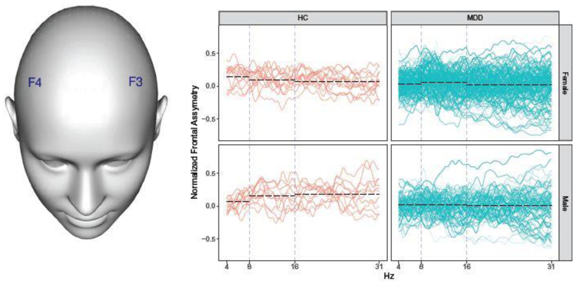
Left: Locations of F3 and F4 electrodes. Right: Normalized frontal asymmetry curves. HC = healthy control, MDD = major depressive disorder. Blue vertical dashed lines separate the theta (4 – 8 Hz), alpha (8 – 16 Hz), and beta (16 – 31 Hz) frequency bands. Black dashed lines show mean values within a frequency band.

The right panels of Figure 1 show the FA curves over the θ, α, and β frequency bands for MDD and HC subjects in the EMBARC study stratified by gender. The FA curves are computed as $\frac{F4(t)-F3(t)}{F4(t)+F3(t)}$ for t ∈[4,31.75] Hz where F4(t) and F3(t) are the CSD power values at frequency t for the F4 and F3 electrodes, respectively. FA values are available at 112 frequencies ranging from 4 to 31.75 Hz in 0.25 Hz increments. An analysis on the scalar summary FαA values similar to that in van der Vinne et al. (2017) is equivalent to comparing the group-mean values corresponding to the dashed black lines over the 8 to 16 Hz band. We propose to fit a functional regression model with the FA curve as the response and diagnostic status as the primary predictor, adjusting for gender, age, and other relevant factors.

Unfortunately, some of the EEG data collected in the EMBARC study were flagged during quality control assessment as being “Unacceptable” or “ Marginal” and therefore should not be used in our analysis. Still others were wholly missing. In fact, Figure 1 displays only those FA curves for subjects with “Acceptable” or “Good” quality control designations. In addition, some of the values for the covariates that we wish to adjust for are missing for some subjects. Instead of throwing out observations from subjects with incomplete data and conducting a complete case analysis, we have developed a multiple imputation (MI) procedure (Rubin 1987; Schafer 1997) for imputing the missing scalar and functional data and propose an approach for pooling estimates derived from the multiply imputed data sets.

MI methods for scalar data have been broadly developed and research in this area remains active, particularly in employing machine learning methods (Doove et al. 2014; Xu et al. 2016; Zhao and Long 2016). Furthermore, there are many user-friendly software packages that perform MI when the data consist only of scalar quantities, including software developed for r (R Development Core Team 2018) such as mice (Buuren and Groothuis-Oudshoorn 2011) and Amelia (Honaker et al. 2011) and procedures developed for sas (SAS Institute Inc 2011) such as PROC MI and PROC MIANALYZE. Similar methods and software should be available for handling functional data. To our knowledge, approaches for MI of functional data have not been investigated in the literature nor has software been developed to perform MI with functional data.

The rest of the paper is structured as follows. In Section 2 we provide an overview of our target analysis models: functional regression models with either functional or scalar outcomes. In Section 3 we extend the missing data framework to include functional data. In Section 4 we present a method for performing MI via chained equations with scalar and functional data. Section 5 presents the results of a simulation study, showing the performance of the proposed imputation and pooling procedures. Section 6 illustrates the proposed method using data from the EMBARC trial. We conclude in Section 7 with a discussion and comments on possible directions for future research. A supplementary appendix includes further detail on fitting functional regression as well as additional simulation and application results.

Throughout, we use the following notational conventions: upper-case bold letters for matrices or collections of functions (distinction should be obvious by context), lower-case bold variables represent vectors, upper-case non-bold Roman letters for functions, lower-case non-bold Roman letters for scalars. Non-bold Greek letters are used for both scalar and functional parameters but the distinction should be obvious by context.

2. Review of Functional Regression Models

Functional regression refers to a broad category of models. If the response is a function and the predictors are functions, scalars, or both, then we refer to these as functional response models (FRMs). If the response is a scalar and the predictors are functions or both functions and scalars, then we refer to these as scalar response models (SRMs). Here, we briefly outline broad classes of FRMs and SRMs and methods for fitting them.

2.1. Functional Response Models (FRMs)

Suppose we collect a sample of n independent observations from a population of interest. For each observation, we have a function designated as the response, denoted by Y_i, p scalar variables, denoted by the p-dimensional vector z_i = (z_i,1, …, z_i,p)^⊤, and q functional variables, denoted by the q-element set of functions X_i ={X_i,1, …, X_i,q } for i = 1, …, n. Assume that Y_i is a one-dimensional functional random variable that is square integrable on a compact support $I_Y\subset ℝ$ (i.e, ${\int }_{I_Y}{Y}_i^2(t)dt<\infty$). Similarly, assume that X_i,1, …, X_i,q are one-dimensional functional random variables that are each square integrable on a compact support $I_k\subset ℝ$ (i.e, ${\int }_{I_k}{X}_{i,k}^2(t)dt<\infty$, k = 1, …, q). For clarity, we assume that the functional predictors are observed without error.

We can model the relationship between the functional response and predictors as:

$$\begin{gathered} Y_i(t)~EF\left({\mu }_i(t),\eta \right),\text{ such that } \\ g\left\{{\mu }_i(t)\right\}={\beta }_0(t)+\sum _{j=1}^p{z}_{i,j}{\beta }_j(t)+\sum _{k=1}^q\int X_{i,k}(s){\rho }_k(s,t)ds. \end{gathered}$$ (1)

In (1), EF(μ_i (t),η) corresponds to an exponential family distribution with mean μ_i(t) and a set of nuisance parameters given by the vector η, g(·) is a link function, β₀(t) is the intercept function, β_j(t) for j = 1, …, p are the coefficient functions corresponding to the functional effects of the scalar predictors on the functional response, and ρ_k (s, t) for k = 1, …, q are the functional effects of the functional predictors on the functional response.

With complete data, there are several methods available for estimating the coefficients in (1). In subsequent sections, we employ a fitting approach described in (Ivanescu et al. 2015) for settings where Y_i(t) are normally distributed and more generally in Scheipl et al. (2016) where Y_i(t) can be from any exponential family distribution. These fitting methods are referred to as penalized function-on-function regression (PFFR).

2.2. Scalar Response Models (SRMs)

Suppose that we observe z_i and X_i for i = 1, …, n as above, but have a scalar response, y_i. We can assume that the model of interest is the generalized functional linear model (McCullagh and Nelder 1989; Cardot et al. 1999):

$$y_i~EF\left({\mu }_i,\eta \right),\text{ such that }g\left({\mu }_i\right)={\theta }_0+z_i\theta +\sum _{j=1}^q\int X_{i,j}(t){\beta }_j(t)dt.$$ (2)

In (2), EF(μ_i, η) corresponds to an exponential family distribution with mean μ_i and dispersion parameter η, g(·) is a link function, θ₀ is the intercept, θ is a p-vector of scalar coefficients, and β_j(t), j = 1, …, q, are square integrable on a compact support.

As with FRMs, there are several methods for estimating SRMs. In the following sections, we consider penalized functional regression (PFR) (Goldsmith et al. 2011) since it is able to handle both scalar and functional predictors as well as generalized scalar outcomes. A brief overview of both the PFFR and PFR fitting procedures is provided in Section 1 of the online Appendix.

3. Missing Scalar and Functional Data

Missing data mechanisms and models have been discussed extensively elsewhere (e.g., Rubin (1987); Little and Rubin (2002); van Buuren (2012)). Here we provide an overview of these concepts in settings with both scalar and functional data as well as an overview of multiple imputation.

3.1. Notation and Missingness Mechanisms

We start by relabeling the scalar and functional variables. If the response of interest is a scalar, then we let y_i = w_i,1, z_i,1 = w_i,2, …, z_i,p = w_i,p+1, and X_i,1 = w_i,p+2, …, X_i,q = w_i,p+q+1. If the response of interest is a function, then we let z_i,1 = w_i,1, …, z_i,p = w_i,p, Yi = w_i,p+1, and X_i,1 = w_i,p+2, …, X_i,q = w_i,p+q+1. Either way, the p + q + 1 variables can be gathered into an n × (p + q + 1) matrix of components, which are a mix of scalars and functions, W = (w₁, …, w_p+q+1). w_i = (w_i,1, …, w_i,p+q+1)^⊤ represents a random draw from a multivariate distribution having a set of unknown parameters denoted by ξ. Let R = (r₁, …, r_p+q+1) be an n × (p + q + 1) indicator matrix with entries r_i,j such that r_i,j =1 if w_i,j is observed and r_i,j = 0 if w_i,j is missing. Let W^obs and W^mis denote the observed and missing components of W, respectively. The expression for the missing data model is P(R|W^obs, W^mis, ψ), where ψ is the collection of model parameters.

The classification of missing data given in Little and Rubin (2002) can be extended to include functional data. Data are missing completely at random (MCAR) if P(R = r|W^obs, W^mis, ψ) = P(R = r|ψ), missing at random (MAR) if P(R = r|W^obs, W^mis, ψ) = P(R = r|W^obs, ψ), or missing not at random (MNAR) if P(R = r|W^obs, W^mis, ψ) does not simplify.

Under MCAR and some MNAR settings (Bartlett et al. 2014), a complete case analysis (CCA) yields unbiased estimates for the model parameters. However, these estimates may be inefficient since incomplete cases are being discarded. When there are many predictors, each prone to missing values, the number of complete cases can be much smaller than the full set of observations. This can greatly limit one’s ability to extract information from data with complex associations.

When data are MAR, a CCA can yield both inefficient and biased parameter estimates in some settings (e.g., if missingness in covariates depends on the value of the response (White and Carlin 2010)). Under MAR mechanism, missing data can be imputed using imputation models that provide predictions for the missing values. The assumption that data are MAR is not testable with available data, but previous work suggests that the MAR assumption is approximately valid if the imputation model includes enough relevant variables (Schafer 1997; Collins et al. 2001; Harel and Zhou 2007; White et al. 2011; Perkins et al. 2018). In the following sections, we assume that the data are MAR. In addition, we also assume that the parameter spaces for ψ and ξ are distinct (i.e., the joint parameter space is equivalent to the product of the individual parameter spaces). The combination of MAR and parameter distinctness allows us to ignore the missingness indicators, R, in likelihood or Bayes-type inferences (Little and Rubin 2002).

3.2. Joint and Imputation Models

Rubin (1987) gives a general framework to conduct imputation of missing data: imputation should follow from the specification of a joint model for [W, R]. Correct specification of such a model can be a complex task in settings with purely scalar data of mixed types (e.g., continuous, categorical, etc.) and is made even more complex here with functional data. Fortunately, we propose that values can be imputed without directly specifying this joint distribution. Instead, one can specify an imputation model, f (W^mis|W^obs, R), that describes how missing values are generated. In MI, one draws from this distribution multiple times to create multiple complete data sets.

Conceptually, MI in settings with both scalar and functional data is similar to MI of purely scalar data. The goal is to use the distribution of the observed data to fill in plausible values for the missing data. As with purely scalar data, here MI can be justified using a Bayesian framework.

Under MAR and ignorability assumptions (and also under the stricter MCAR assumption) the posterior predictive distribution for W^mis is independent of R and given by

$$f\left(W^{mis}\mid W^{obs}\right)=\int f\left(W^{mis}\mid W^{obs},\xi \right)f\left(\xi \mid W^{obs}\right)d\xi ,$$ (3)

where f (W^mis |W^obs, ξ) is the predictive distribution of W^mis given W^obs and ξ,

$$f\left(\xi \mid W^{obs}\right)\propto f(\xi )\int f\left(W^{mis},W^{obs}\mid \xi \right)d{W}^{mis},$$ (4)

is the observed-data posterior distribution for ξ, and f (ξ) is the prior distribution. Together, (3) and (4) point to a two-step method for MI: in the m-th imputation (m = 1, …, M), first make a random draw for ξ from its posterior distribution, denoted by ξ^(m), then impute the missing values in W_mis by a random draw from f (W^mis|W^obs, ξ^(m)) to obtain W ^mis(m).

4. Multiple Imputation for Scalar and Functional Data

4.1. Imputation Procedures

4.1.1. Simplified Case

For the sake of clarity, we begin by considering settings in which all but one variable, w_·j (here the ·j subscript indicates column j of matrix W), are completely observed. Without loss of generality, assume that the first r values in w_·j are observed, denoted by $w_{\cdot j}^{obs}={\left(w_{1,j},\dots ,w_{r,j}\right)}^{\top }$, and the last n – r values in w_·j are missing, denoted by $w_{\cdot j}^{mis}={\left(w_{r+1,j},\dots ,w_{n,j}\right)}^{\top }$. Define the complement data set to w·j by $W_{-j}=\left(w_1,\dots ,w_{\cdot j-1},w_{\cdot j+1},\dots ,w_{\cdot p+q+1}\right)={\left[W_{-j}^{obs\top },W_{-j}^{mis\top }\right]}^{\top }$.

The observed data are $W^{obs}=\left\{w_j^{obs},W_{-j}^{obs},W_{-j}^{mis}\right\}$ and the missing data are $W^{mis}=w_{\cdot j}^{mis}$ so that there are r complete observations and n – r incomplete observations that are missing values for w_·j. In this setting, the imputation model in (3) can be expressed as $f\left(w_{\cdot j}^{mis}\mid w_{\cdot j}^{obs},W_{-j}\right)=\int f\left(w_{\cdot j}^{mis}\mid W_{-j}^{mis},{\xi }_j\right)f\left({\xi }_j\mid w_{\cdot j}^{obs},W_{-j}^{obs}\right)d{\xi }_j$. In order to obtain the posterior distribution $f\left({\xi }_j\mid w_{\cdot j}^{obs},W_{-j}^{obs}\right)$, we can specify and fit a regression model with $w_{\cdot j}^{obs}$ as the response and $W_{-j}^{obs}$ as the predictors.

When w_·j is one of the scalar variables (e.g., w_i,j = z_i,j or y_i when the analysis model is a SRM), we can employ a suitable SRM. For example, we use the model z_i,j ~ EF(μ_i,j, η_j) such that,

$$\begin{gathered} h_j\left({\mu }_{i,j}\right)={\gamma }_{j,0}+\sum _{\ell \ne j}{z}_{i,\ell }{\gamma }_{j,\ell }+{\alpha }_j{y}_i+\sum _{k=1}^q\int X_{i,k}(t){\omega }_{j,k}(t)dt\text{ or } \\ {h}_j\left({\mu }_{i,j}\right)={\gamma }_{j,0}+\sum _{\ell \ne j}{z}_{i,\ell }{\gamma }_{j,\ell }+\int {\alpha }_j(t)Y_i(t)dt+\sum _{k=1}^q\int X_{i,k}(t){\omega }_{j,k}(t)dt, \end{gathered}$$ (5)

depending on whether the response for the analysis model is a scalar (top) or a function (bottom). The components of (5) are similar to those in analysis model (2) where the collection of parameters is ξ_j ={γ _j,0, γ _{j,ℓ(ℓ ≠ j)}, α_j, ω_j,1, …, ω_j,q}, which can be estimated using PFR or any other suitable approach. When the error function corresponds to either the binomial or Poisson distributions, the ith subject’s missing value for the jth variable is imputed with a random draw from either distribution, using the predicted value of μ_i,j. When the error function is normal, the missing value is imputed with the predicted value of μ_i,j with a random error term added. This error term is drawn from the $N\left(0,{\widehat{\sigma }}_j^2\right)$ distribution, where ${\widehat{\sigma }}_j^2$ is estimated from the residuals under model (5).

When w_·j is a functional variable (e.g., w_i,j = X_i,j or Y_i when the analysis model is a FRM), we can employ a suitable FRM. For example, we use the model X_i,j (t) ~ EF(μ_i,j (t), η_j) such that,

$$\begin{array}{l}{h}_j\left\{{\mu }_{i,j}(t)\right\}={\gamma }_{j,0}(t)+\sum _{\ell =1}^p{z}_{i,\ell }{\gamma }_{j,\ell }(t)+y_i{\alpha }_j(t)+\sum _{k\ne j}\int X_{i,k}(s){\omega }_{j,k}(s,t)ds\text{ or }\\ h_j\left\{{\mu }_{i,j}(t)\right\}={\gamma }_{j,0}(t)+\sum _{\ell =1}^p{z}_{i,\ell }{\gamma }_{j,\ell }(t)+\int Y_i(s){\alpha }_j(s,t)ds+\sum _{k\ne j}\int X_{i,k}(s){\omega }_{j,k}(s,t)ds,\end{array}$$ (6)

depending on whether the response for the analysis model is a scalar (top) or a function (bottom). The components of (6) are similar to those in analysis model (1) and the collection of parameters ξ_j = {γ_j,0, γ_j,1, …, γ_j,p, α_j, ω_{j,k(k ≠ j)}} can be estimated using PFFR or any other suitable approach. When the error function corresponds to either the binomial or Poisson distribution, the ith subject’s missing value for the jth variable at domain value t can be filled in with a random draw from either distribution, using the predicted value of μ_i,j (t). When the error function is normal then the ith subject’s missing value for the jth covariate at domain value t can be filled in with the predicted value of μ_i,j (t) with a functional error term added to it. This functional error term is generated as follows. First, we compute estimates of the leading principal component basis functions $\left\{{\widehat{\psi }}_1,\dots ,{\widehat{\psi }}_K\right\}$ (accounting for at least 99% of the variance), the corresponding score variances, $\lambda ={\left({\widehat{\lambda }}_1,\dots ,{\widehat{\lambda }}_K\right)}^{\top }$, and mean function, ${\widehat{\mu }}_r$, from a functional principal components decomposition of the collection of residual curves derived from fitting (6) on the observations for which the jth covariate is observed. Then we generate subject-specific principal component loadings, c_i = (c_1,i, …, c_K,i)^⊤, from c_i ~ N(0,diag(λ)), and let $r_i(t)={\widehat{\mu }}_r(t)+\sum _{k=1}^K{c}_{ki}{\widehat{\psi }}_k(t)$ be the functional error term for the ith subject.

In order to account for uncertainty in the imputation model parameters, we propose to select a bootstrap sample from the complete data and obtain parameter estimates from fitting (5) or (6) on the bootstrap sample. The use of a bootstrap sample is suggested in van Buuren (2012) Section 3.1. The complete procedure is repeated M times to obtain M imputed data sets. Both (5) and (6) can be made more flexible by the addition of various interaction terms or by allowing for less restrictive functional forms for the coefficient functions. These modifications may increase the computational complexity of the imputation procedure.

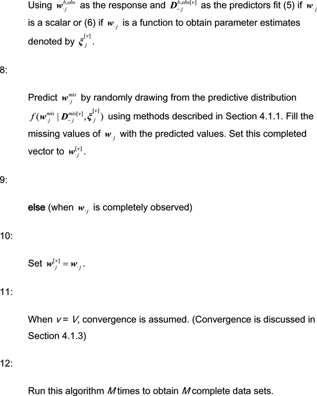
4.1.2. General Missing Patterns and the fregMICE Algorithm

When more than one variable are incomplete, we propose to employ an extension of multiple imputation by chained equations (MICE) (van Buuren and Oudshoorn 1999) that incorporates functional variables. MICE is conducted in a variable-by-variable manner via specification of a conditional model for each w_·j (j = 1, …, p + q + 1) given by f (w_·j| W_−j, R, ξ_j). The proposed functional regression MICE (fregMICE) algorithm is provided in Algorithm 1. We assume that the variables are arranged such that those with the least missing data have lower index values (j) and those with more missing data have higher index values. As with the original MICE procedure, any pattern of missingness in the variables can be accommodated. The fregMICE Algorithm can be run in parallel with M streams yielding M imputed data sets after V iterations.

4.1.3. Convergence and Diagnostics for the fregMICE Procedure

In settings with only scalar data, it is common to assess convergence of the MICE procedure via inspection of plots of selected parameters that summarize the imputed data (e.g., mean or standard deviation of the imputed values) vs. iteration number for each of the M parallel sequences. When the specified values for the parallel sequences are plotted together, the streams should overlap and be free of trend in order to diagnose convergence (van Buuren and Oudshoorn 1999). If a stream trails off, away from the other streams, or shows systematically different variation from the other streams, then this would suggest convergence issues for that stream. We propose to use the same assessment techniques for imputations of scalar values generated from our fregMICE procedure and similar techniques for the imputations of functional values. Specifically, for the imputed function values, we propose to plot point-wise summary parameters (e.g., mean or standard deviation) for each iteration of each parallel sequence. We will diagnose convergence if the plots are free of trend and show adequate overlap across the streams. As with scalar imputation, if a sequence of curves in a stream trails off (either the entire function or over a restricted domain) relative to the other streams or the sequence of curves shows systematically different variation from the other streams, then this would suggest convergence issues for that stream.

Aside from assessing convergence, one may also want to assess the fidelity of the imputed values to those observed in the data set. One way to do this is to create strip-plots. For imputed scalar data, these plots show the observed and imputed values from each imputed data set in contrasting colors. This allows one to easily identify whether imputed values are realistic and can help the analyst decide if the imputation model needs to be adjusted. Strip plots can also be constructed for imputed functional data and can be used to make similar assessments. We illustrate these strip plots and convergence plots in our application in Section 6 and in the supplementary Appendix.

4.2. Analysis of Multiply Imputed Datasets

The generation of multiple data sets accounts for the inherent uncertainty in the prediction of the missing values. Once the imputed data sets are constructed, we analyze each one using a method designed for complete data. Most methods for estimating functional regression models, including the PFFR and PFR approaches that we employ in subsequent sections, represent the coefficient functions using judiciously selected sets of basis functions and then estimate the corresponding basis coefficients. Specifically, for model (1), we let ${\beta }_j(t)=B_j^{\top }(t)b_j$ for j =0, …, p, where $B_j(t)={\left(B_{j,1}(t),\dots ,B_{j,L_j}(t)\right)}^{\top }$ is a vector of basis functions for β_j(t) and $b_j={\left(b_{j,1},\dots ,b_{j,L_j}\right)}^{\top }$ is the corresponding vector of unknown basis coefficients. Similarly, we let ${\rho }_k(s,t)=U_k^{\top }(s,t)u_k$, for k = 1, …, q, where $U_k(s,t)={\left(U_{k,1}(s,t),\dots ,U_{k,L_k}(s,t)\right)}^{\top }$ is a vector of bivariate basis functions (e.g., bivariate thin-plate splines) selected for ρ_k(s,t) and $u_k={\left(u_{k,1},\dots ,u_{k,L_k}\right)}^{\top }$ is the corresponding vector of unknown basis coefficients. The coefficient functions in (2) can be represented similarly.

The fitted models from the M imputed data sets can be pooled to provide coefficient and variance estimates that account for both within and between imputation variability. We will use the variance estimates to construct approximate confidence intervals for the scalar coefficients and point-wise confidence bands for the coefficient functions.

Rubin’s Rules (Rubin 1987) provide a method for combining scalar and multivariate estimates after MI and can be extended to settings involving functional data. For clarity, we illustrate the pooling approach for estimating the univariate functional coefficient parameters in model (1).

Let ${\widehat{\beta }}_j^{(m)}(t)=B_j^{\top }(t)b_j^{(m)}$ be the estimate of β_j (t) from the m^th imputed data set. The pooled point estimate for β_j (t) is given by ${\overline{\beta }}_{j,M}(t)=\frac{1}{M}\sum _{m=1}^M{B}_j^{\top }(t)b_j^{(m)}=B_j^{\top }(t)\left\{\frac{1}{M}\sum _{m=1}^M{b}_j^{(m)}\right\}=B_j^{\top }(t){\overline{b}}_{j,M}$. The total variance of ${\overline{\beta }}_{j,M}(t)$ should incorporate both within and between-imputation variability. Let ${\widehat{V}}_j^{(m)}(t)=var\left\{{\widehat{\beta }}_j^{(m)}(t)\right\}=var\left\{B_j^{\top }(t)b_j^{(m)}\right\}=B_j^{\top }(t)var\left(b_j^{(m)}\right)B_j(t)=B_j^{\top }(t){\widehat{\Lambda }}_{b_j}^{(m)}{B}_j(t)$, where ${\widehat{\Lambda }}_{b_j}^{(m)}$ is the estimated covariance matrix of $b_j^{(m)}$. With ${\widehat{V}}_j^{(m)}\left(t\right)$ defined, we have the mean within-imputation variance given by ${\overline{V}}_{j,M}(t)=\frac{1}{M}\sum _{m=1}^M{\widehat{V}}_j^{(m)}(t)=\frac{1}{M}\sum _{m=1}^M{B}_j^{\top }(t){\widehat{\Lambda }}_{b_j}^{(m)}{B}_j(t)=B_j^{\top }(t)\left\{\frac{1}{M}\sum _{m=1}^M{\widehat{\Lambda }}_b^{(m)}\right\}{B}_j(t)=B_j^{\top }(t){\overline{\Lambda }}_{b_j,M}{B}_j(t)$, and between-imputation variability given by $B_{j,M}(t)=\frac{1}{M-1}\sum _{m=1}^M{\left\{{\widehat{\beta }}_j^{(m)}(t)-{\overline{\beta }}_{j,M}(t)\right\}}^2=\frac{1}{M-1}\sum _{m=1}^M{\left\{B_j^{\top }(t)\left(b_j^{(m)}-{\overline{b}}_{j,M}\right)\right\}}^2$ where ${\overline{\Omega }}_{j,M}=B_j^{\top }(t)\left\{\frac{1}{M-1}\sum _{m=1}^M{\left(b_j^{(m)}-{\overline{b}}_{j,M}\right)}^{\top }\left(b_j^{(m)}-{\overline{b}}_{j,M}\right)\right\}{B}_j(t)=B_j^{\top }(t){\overline{\Omega }}_{j,M}{B}_j(t)$ is the covariance matrix quantifying the variability in the estimated basis coefficients between imputations. The total variance of ${\overline{\beta }}_{j,M}(t)$ is then given by ${\overline{V}}_{j,M}(t)+\left(1+\frac{1}{M}\right)B_{j,M}(t)$, comprising contributions from variability within and between the imputed data sets. We propose to construct an approximate 95% confidence interval for β_j (t₀) using ${\overline{\beta }}_{j,M}\left(t_0\right)\pm 1.96\sqrt{{\overline{V}}_{j,M}\left(t_0\right)+\left(1+\frac{1}{M}\right)B_{j,M}\left(t_0\right)}$.

It is straightforward to construct pooled estimators and corresponding variances for the bivariate coefficient functions, ${\rho }_k^{(m)}(s,t)$ for k = 1, …, q, in model (1). One can also use these procedures to obtain estimators and corresponding variances for coefficient functions in model (2) and use the standard methods proposed in Rubin (1987) for the scalar coefficients.

5. Simulation Study

Here we investigate the performance of fregMICE algorithm and evaluate the characteristics of the pooled estimators and approximate confidence intervals proposed in the previous section. The simulation settings were designed to be similar to those encountered in the EMBARC data. As there are no other methods in the literature to deal with these settings, we compare our fregMICE algorithm to mean imputation and CCA.

5.1. Data Generation

Our simulation study focuses on settings with a functional response, Y, and its association with three scalar predictors, z₁, z₂, and z₃. We generated z_1i ~ Bin(1,0.4) and (z_2i, z_3i) ~ N((2,0), $\left(\begin{array}{cc}1& 0.6\\ 0.6& 1\end{array}\right)$) for i = 1, …, 350. We selected n = 350 since this is close to the number of subjects in our application. (Results for n = 100 are provided in Appendix Section 2.) The functional outcome is observed on a grid $\left\{t_g=\frac{g}{10}:g=0,1,\dots ,100\right\}$ on the interval [0,10] and related to the scalar predictors via the equation,

$$Y_i(t)={\beta }_0(t)+{\beta }_1(t)z_{1i}+{\beta }_2(t)z_{2i}+{\beta }_3(t)z_{3i}+{\epsilon }_i(t),$$ (7)

where we consider two sets of true coefficient functions. For the first set, which we refer to as “Parameter Set 1,” we have ${\beta }_0(t)=0.25t$, ${\beta }_1(t)=\text{sin}\left(\frac{\pi t}{10}\right)$, ${\beta }_2(t)=0.3e^{t/5}$, and ${\beta }_3(t)=-0.2sin\left(\frac{\pi t}{10}\right)$. For the second set, which we refer to as “Parameter Set 2,” we have ${\beta }_0(t)=0.25t$, ${\beta }_1(t)=\text{sin}\left(\frac{\pi t}{5}\right)$, ${\beta }_2(t)=\frac{2}{\sqrt{2\pi }}{e}^{-{(t-2)}^2/2}$, ${\beta }_3(t)=\frac{-1}{\sqrt{2\pi }}\left\{e^{-{(t-2)}^2/2}+e^{-{(t-8)}^2/2}\right\}$. β₁, β₂, and β₃ in Parameter Set 2 have more localized features relative to Parameter Set 1 and are therefore more challenging to estimate using the PFFR approach. In each setting, ε_i(t) is simulated from a Gaussian process with mean zero and covariance V (s,t) = 4·0.15^|s−t| + 0.05² · I(s = t) where I (s = t) is 1 if s = t and 0 otherwise. Figure 2 shows simulated responses generated under Parameter Sets 1 and 2.

Fig. 2.

50 simulated responses from Parameter Set 1 with three highlighted observations (Left). 50 simulated responses from Parameter Set 2 with three highlighted observations (Right).

For each set of parameters, we consider two scenarios. In Scenario (a), only z₂ has missing values and in Scenario (b), both z₂ and Y have missing values. In both Scenarios (a) and (b), z₁ and z₃ are fully observed and the probability that z₂ is observed is given by $\mathit{\text{logit}}\left\{P\left(R_{z_{2i}}=1\right)\right\}={\alpha }_0-20I\left\{s_i>{\alpha }_1\right\}+{\alpha }_2\frac{1}{1+e^{-z_{1i}}}+{\alpha }_3\frac{1}{1+e^{-z_{3i}}}$ for observation i where $s_i=\sum _{g=0}^{100}{Y}_i\left(t_g\right)$. In Scenario (a), where Y is always observed, we set α₀ = 10, α₂ = α₃ =0, and let α₁ be the 90th, 80th, or 70th percentile of {s₁, …, s₃₅₀} so as to achieve exactly 10%, 20%, or 30% missingness in z₂ respectively. In Scenario (b), whether z₂ is observed depends only upon the values of z₁ and z₃ such that α₁ = max{s₁, …, s₃₅₀} (so that missingness is independent of Y), α₂ = 1, α₃ = −1 and α₀ = 2.1,1.3, or 0.8 to achieve about 10%, 20%, or 30% missingness in z₂ respectively. Also for Scenario (b), the probability that Y is observed is given by $\mathit{\text{logit}}\left\{P\left(R_{Y_i}=1\right)\right\}={\psi }_0+{\psi }_1\frac{1}{1+e^{-z_{1i}}}+{\psi }_2\frac{1}{1+e^{-z_{3i}}}$ where ψ₁ = −1, ψ₂ = 1, and ψ₀ = 2.3,1.5, or 0.9 to achieve about 10%, 20%, or 30% missingness in Y respectively. The mean (sd) proportions of missing values and complete cases realized in the simulation study are provided in Section 2 of the Appendix. We note that the proportion of complete cases in the EMBARC application is about 61%, while the proportions of complete cases in our simulation studies range from 49% to 90%. We generated 500 data sets under each parameter set, scenario, and missingness combination.

In Scenario (a), z₂ values are MAR with missingness depending on the response, Y, in such a way that observations with missing data have functional responses that tend to have larger values across the domain [0,10]. In this scenario, it is expected that CCA will yield biased estimates. In Scenario (b), z₂ values are MAR with missingness depending only on the other covariates, but not the response. The response, Y, is also MAR. In this scenario, CCA is not expected to be biased.

5.2. Procedures Compared and Performance Measures

For each simulation setting, we fit the correctly specified model for Y using PFFR where each coefficient function was represented via 20 cubic B-splines and smoothness in the estimated coefficient functions was achieved via a penalty on the magnitude of the second derivative. Smoothing parameters were estimated via restricted maximum likelihood estimation.

As a benchmark, we used all of the data, prior to imposing missingess on any of the variables to fit model (7). In the results, we refer to this as “all no missing” (ANM). For mean imputation, we filled in missing z₂ values with the mean of the observed z₂ values and for missing Y functions, we filled in the point-wise mean function of the observed Y functions. We then used the mean-imputed dataset to fit model (7). For CCA, the analysis model was fit on observations with complete data. For our fregMICE procedure, the imputation model for z₂ was E(z₂|z₁, z₃, Y) = γ₀ + γ₁z₁ + γ₂z₃ + ∫Y(t)ω(t)dt. To estimate this model, we used PFR. In the PFR fitting procedure, functional observations were represented using functional principal components (FPCs) by smoothed covariance (Yao et al. 2003) where the number of FPCs was selected to be the minimum number of components explaining at least 99% of the variance in the functional observations. The coefficient function, ω, was represented using a basis of 30 thin-plate regression splines and the fitting procedure penalized the magnitude of the second derivative. In scenarios where Y had missing values, the imputation model for Y was the same as (7). To estimate this model, we used the correctly specified analysis model fit via PFFR, using 20 cubic B-splines to represent each coefficient function and penalized the magnitude of the second derivative. We ran the fregMICE procedure for 20 iterations and constructed 5 imputed data sets. We fit model (7) on each imputed data set and used the extension of Rubin’s rules described in Section 4.2 to pool estimates from the 5 data sets. Regardless of the method used to handle missing data, we used the pffr function from the refund package (Goldsmith et al. 2018) to fit the analysis model. This function provides different estimates for the covariance matrix that are useful for constructing confidence intervals. In our simulations and application, we employ the Bayesian posterior covariance matrix (Ruppert et al. 2003) which was also used in Ivanescu et al. (2015).

For each coefficient function (β_j (t) for j = 0,1,2, and 3), we show point-wise standardized bias (pwSB) plots. The pwSB was calculated as $SB\left(t_g\right)=\frac{{\overline{\widehat{\beta }}}_j\left(t_g\right)-{\beta }_j\left(t_g\right)}{sd\left\{{\widehat{\beta }}_j\left(t_g\right)\right\}}$, where ${\overline{\widehat{\beta }}}_j\left(t_g\right)$ is the average of the 500 estimates of β_j (t_g) and $sd\left\{{\widehat{\beta }}_j\left(t_g\right)\right\}$ is the Monte-Carlo standard deviation of the estimates. We also provide plots of across-the-function mean point-wise coverage (pwCov) and mean point-wise width (pwWidth) for the estimated 95% confidence bands for each coefficient function by taking the mean coverage and width, respectively, over all t_g values and then averaging over the 500 simulation runs. Additional results are presented in Appendix Section 2.

5.3. Results

Parameter Set 1 Results:

Figure 3 (Top) shows that, for Scenario (a), pwSB for fregMICE and ANM estimates are similar while estimates based on CCA and mean imputation show considerable bias for each coefficient function. The degree of bias is considerably greater for mean imputation. Bias for both mean imputation and CCA increases as the amount of missing data increases, whereas bias is relatively stable for fregMICE. Mean pwCov and pwWidth, for Scenario (a), are shown in the top left of Figure 4. Mean pwCov for fregMICE and ANM are similar, though the intervals tend to be slightly wider for fregMICE, especially as the amount of missing data increases. Coverage decreases substantially and width increases slightly for intervals for β₂ from CCA and mean imputation as the amount of missing data increases. Coverage is poor for intervals derived via the mean imputation procedure.

Fig. 3.

Point-wise standardized bias curves in Setting 1 Scenario (a) (Top) and Setting 1 Scenario (b) (Bottom). Columns (left to right) correspond to 10, 20, and 30% missing data. Rows (top to bottom) correspond to functional parameters β₀, β₁, β₂, and β₃.

Fig. 4.

Across-the-function mean point-wise 95% confidence interval coverage and width for all combinations of Parameter Settings 1 & 2, Scenarios (a) & (b), and missingness. Error bars are ± Monte Carlo standard deviation.

Figure 3 (Bottom) shows that, for Scenario (b), pwSB for fregMICE and ANM estimates are similar. CCA estimates also perform similarly to ANM. This is expected since missingness in both Y and z₂ depends on the completely observed covariates, z₁ and z₃. pwSB is large for estimates based on mean imputation. Mean pwCov and pwWidth, for Scenario (b), are shown in the top right of Figure 4. ANM, fregMICE, and CCA are similar with respect to pwCov but both fregMICE and CCA have greater pwWidths that increase with larger amoutns of missing data. Again, coverage is poor for intervals based on mean imputed data.

Parameter Set 2 Results:

Figure 5 (Top) shows that, for Scenario (a), pwSB for fregMICE and ANM estimates are similar with slight increases for fregMICE with increasing amounts of missing data. CCA and mean imputation-based estimates show considerable bias for each coefficient function across all amounts of missingness. Mean pwCov and pwWidth, for Scenario (a), are shown in the bottom left of Figure 4. Mean pwCov for fregMICE and ANM are similar, though the intervals tend to be wider for fregMICE, especially as the amount of missing data increases. Mean pwCov of β₁ for CCA is similar to ANM, but coverage of the other functional coefficients is lower, especially for β₂ and β₃. Coverage is poor for intervals based on mean imputed data.

Fig. 5.

Point-wise standardized bias curves in Setting 2 Scenario (a) (Top) and Setting 2 Scenario (b) (Bottom). Columns (left to right) correspond to 10, 20, and 30% missing data. Rows (top to bottom) correspond to functional parameters β₀, β₁, β₂, and β₃.

Figure 5 (Bottom) shows that, for Scenario (b), pwSB for fregMICE and ANM estimates are similar. CCA estimates also perform similarly to ANM. As noted above, this is expected since missingness in both Y and z₂ depends only on the completely observed covariates, z₁ and z₃. pwSB is large for estimates based on mean imputation. Mean pwCov and pwWidth, for Scenario (b), are shown in the bottom right of Figure 4. While coverage is similar for ANM, CCA, and fregMICE, the mean pwWidths for CCA and fregMICE are larger and increase with larger amounts of missing data. Again, coverage is poor for intervals based on mean imputed data.

Results Summary:

The fregMICE procedure performs simialrly to the best case scenario where all data are available. It also performs at least as well as or much better than CCA and mean imputation. Though CCA should be unbiased in settings where missingness is independent of the outcome, fregMICE still tends to perform as well or slightly better on the reported performance measures. Across all settings, mean imputation performs poorly in all respects and we recommend against its use. We provide additional results for these settings, as well as for settings where n = 100, in Appendix Section 2. There, we also discuss results from a different set of simulations where the analysis model has a scalar outcome and functional and scalar predictors.

6. Assessing the Association between FA and Depression

In Section 1, we stated that our goal is to use the EMBARC data to characterize the association between FA and MDD status. van der Vinne et al. (2017) suggest that analysis of FA should adjust for both age and gender and consider their potential modifying effects. Kaiser et al. (2018) suggest controlling for handedness (left vs. right) and cognition (mental ability). We follow these suggestions in formulating the functional response analysis model:

$$F{A}_i(t)={\beta }_0(t)+AG{E}_i{\beta }_1(t)+EH{I}_i{\beta }_2(t)+\mathit{\text{WASI}}{V}_i{\beta }_3(t)+MD{D}_i{\beta }_4(t)+SE{X}_i{\beta }_5(t)+MD{D}_i\times SE{X}_i{\beta }_6(t)+MD{D}_i\times AG{E}_i{\beta }_7(t)+{\epsilon }_i(t),$$ (8)

where ε_i (t) ~ N(0, σ²). In model (8), FA_i is the normalized CSD asymmetry curve (see Figure 1) for subjects having EEG data with “Good” or “Acceptable ” quality designations. AGE_i is the mean-cetered age in years (i.e., AGE_i = 0 corresponds to the mean age in the sample of 37.16 years), EHI_i is the Edinburgh Handedness Inventory score (ranging from −100 to 100; completely left to right-handed, respectively), WASIV_i is the raw score for the verbal component of the Wechsler Abbreviated Scale of Intelligence (a measure of cognitive ability with higher values indicating better performance; values range from 20 to 80), MDD_i indicates disease status (1 = MDD, 0 = HC), and SEX_i indicates sex (1 = Female, 0 = Male). (Note that we are breaking with our notation convention and using words with non-bold capital letters to represent scalar quantities.)

Table 1 shows summary statistics by diagnostic group. WASIV is missing for 49 subjects. EEG data are missing for 11 subjects. Among the remaining 324 subjects with EEG data available, 88 have data that are “Marginal” or “ Unacceptable.” We treat these EEG data as missing.

Table 1.

Summary statistics for variables in the analysis model by disease status.

	HC (n = 40)		MDD (n = 295)
Variable	n Available	Mean (SD) or n (%)	n Available	Mean (SD) or n (%)
AGE	40	37.62 (14.85)	295	37.10 (13.29)
EHI	40	70.76 (51.43)	295	71.58 (48.23)
WASIV	35	67.40 (7.29)	251	63.62 (9.59)
QIDS	40	1.40 (1.30)	295	18.08 (2.81)
SEX (Female)	40	25 (62.5)	295	193 (65.4)
FA	39		285
Good		17 (42.5)		126 (42.7)
Acceptable		5 (12.5)		88 (29.8)
Marginal		14 (35.0)		44 (14.9)
Unacceptable		3 (7.5)		27 (9.2)
Missing		1 (2.5)		10 (3.4)

A CCA approach for fitting model (8) uses 204 (60.9%) complete observations. As an alternative, we used our fregMICE method to impute the missing WASIV scores and FA functions. To allow for interaction between diagnostic group and each covariate in the imputation models, we imputed the missing values separately within the HC (n_HC = 40) and MDD (n_MDD = 295) groups, thus making the imputation models more general than the analysis model. The imputation model for the WASIV variable had the same form given in (5) with age, sex, EHI, diagnostic status, and FA curves as predictors as well as QIDS score, a measure of depressive symptomatology available for all subjects. We employed PFR to fit the WASIV imputation model with settings similar to those outlined in Section 5.2. The only difference is that we chose to represent the unknown coefficient functions with a set of 30 B-spline basis functions. The imputation model for the FA variable was similar to model (8) with the additional QIDS score predictor. We employed PFFR to fit this model and used the same settings outlined in Section 5.2. We generated 20 imputed data sets, running the fregMICE Algorithm for 20 iterations to obtain each imputed data set.

Diagnostic convergence and strip plots are provided and discussed in Appendix Section 3. Overall, we saw no reason to doubt the adequacy of the imputed FA curves for either the HC or MDD groups. There were several instances in which the imputed WASIV scores were higher than the maximum possible score of 80. These scores were set to 80 prior to fitting the analysis model.

We combined the m^th imputed data sets for the HC and MDD subsets for m=1,…20 to obtain 20 complete data sets. We fit model (8) on each of the 20 complete imputed data sets via PFFR using the same settings as the imputation model for the FA curves described above. Results were pooled and approximate 95% point-wise confidence bands were calculated according to Section 4.2. As in Section 5.2, we used the Bayesian posterior covariance matrix of the estimated basis coefficients to obtain point-wise standard errors for the estimated coefficient functions.

Figure 6 shows the pooled functional coefficient estimates and corresponding 95% point-wise confidence bands for model (8) as well as estimates and confidence bands derived from CCA and from the mean-imputed data. Most fregMICE coefficient estimates are similar to those derived from CCA, but with considerably wider point-wise confidence bands. Coefficient estimates from the mean-imputed data tend be closer to 0 across most functions in comparison to the fregMICE and CCA estimates. Inspection of the estimates from each of the 20 imputed data sets (not shown here) reveals that the wide widths of the confidence bands around the fregMICE estimates are due to the relatively large amount of between imputation variance. This is not surprising considering the HC sample was small with only 22 subjects having “Good” or “Acceptable” quality EEG data.

Fig. 6.

Coefficient function estimates from CCA, fregMICE, and mean imputation.

From the coefficient plots in Figure 6 we see evidence of differences in the FA curves between the MDD and HC groups that depend on both sex and age. The dependence on sex and age is more pronounced with the CCA estimates whose point-wise confidence bands are narrower. To better understand how the differences between the MDD and HG groups depend on both sex and age, we constructed plots of the model-based mean FA curves for different combinations of the predictor values. We provide a Shiny app, available in the Supplementary Materials, to do this.

Figure 7 shows one set of plots in which the mean FA curves for MDD and HC subjects are stratified by sex for three different age values corresponding to the mean age in the sample (37.16), one standard deviation below (23.70), and one standard deviation above (50.62). For all plots, EHI and WASIV were set to their sample mean values of 71.48 and 64.08 respectively. Both the CCA and fregMICE estimates show that, among females, HC subjects tend to have greater FA than MDD subjects at a younger age across most frequency values, but that the difference between the groups decreases with age and ultimately the difference reverses direction with older female MDD subjects having greater FA, primarily in the θ and α frequency bands. For males, the plots for both the CCA and fregMICE estimates show that HC subjects tend to have greater FA than MDD subjects at a younger age and that difference persists, though slightly diminished, in the late α and β frequency bands at older ages. In the θ and early α bands, the difference diminishes with increasing age and ultimately reverses with older male MDD subjects showing greater FA in the θ and early α bands than older male HC subjects. In contrast to CCA and fregMICE, the coefficient estimates derived from mean imputation show similar patterns of difference between the HC and MDD groups for both males and females and across different ages. This follows from the fact that the coefficient estimates for the interaction terms (${\widehat{\beta }}_6$ and ${\widehat{\beta }}_7$) based on mean imputation are closer to zero than estimates from either CCA or fregMICE.

Fig. 7.

Model-based mean FA curves from CCA, fregMICE, and mean imputation. Curves are given for three AGE values (mean age in the sample (37.16), one standard deviation below (23.70), and one standard deviation above (50.62)) with EHI = 71.48 and WASIV = 64.08 (the sample means for each variable).

7. Discussion

In this article, we make two main contributions. First, we have provided a more complete examination of the relationship between frontal power asymmetry and MDD than is currently available in the clinical literature. We employ a functional data analytic approach that allows for differential association with age and sex, while accounting for cognitive ability and handedness. Few previous studies have had sample sizes that were large enough to allow for estimation of these age and sex-specific associations. By employing a functional response model, we were able to investigate differences in frontal asymmetry over a range of frequency values, thus providing a richer characterization of differences between healthy control subjects and those with MDD than is typically available when scalar summary values are used to quantify frontal asymmetry. While most previous studies have focused on using frontal α asymmetry (a scalar value corresponding to the average asymmetry over the α frequency band), our results suggest that frequency values outside of the α-band may hold promise in serving as biomarkers for MDD. For example, our results showed relatively large differences in frontal power asymmetry over the θ frequency band for younger females and over the β frequency band for males across a wide range of ages. It may prove valuable to investigate whether these differences appear in other samples of MDD and healthy control subjects.

Secondly, we have extended the MICE algorithm and Rubin’s rules so that they can be applied in settings that involve both scalar and functional data. Research on handling missing data in FDA is extremely limited (Preda et al. 2009; He et al. 2011; Febrero-Bande et al. 2019). To our knowledge, CCA is the current state-of-the-art when entire functional values are missing. As in the purely scalar setting, CCA is not a universally acceptable approach. Our simulations show that, in some settings, CCA leads to greater bias in parameter estimates and correspondingly poor coverage for point-wise confidence bands when compared to the fregMICE procedure. Our proposed extensions to existing multiple imputation methods do have several limitations. First, as in the completely scalar case, the MAR assumption should hold in order for the proposed methods to yield unbiased estimates of the parameters of interest. Potthoff et al. (2006) discuss this issue and propose techniques for assessing the MAR assumption. For MNAR cases, more complex imputation models, which include joint modeling of data and missingness, are needed. Second, it is clear that the imputation models should be specified so as to provide high-quality imputations. This becomes a complex task in settings with many scalar and functional variables. New robust methods will need to be developed to handle missing data in such settings. Third, the fregMICE procedure is computationally intensive. Though the computational burden does not prohibit its use in settings with a handful of variables (e.g., 5 to 10 scalar and functional variables), it may require more advanced computing capacity in settings with many scalar and functional variables with high rates of missingness. Such settings will likely arise as biomedical and public health research studies collect greater amounts of both scalar and functional variables. New approaches that increase computational efficiency will need to be developed. Fourth, as we noted in Section 4.1.3, checking convergence of the standard MICE procedure tends to rely on ad hoc approaches like inspection of various convergence plots of summary measures. While we employed a similar approach in our application via plotting the point-wise mean of the imputed functions at each iteration, it may be instructive to consider other summary measures (e.g., cross-covariance, measures of smoothness, etc.) or methods to assess convergence.

References

- American Psychiatric Association (2013). Diagnostic and statistical manual of mental disorders (5th ed.) American Psychiatric Association, Washington, DC. [Google Scholar]
- Bartlett J, Carpenter J, Tilling K, and Vansteelandt S (2014). Improving upon the efficiency of complete case analysis when covariates are mnar. Biostatistics 15:719–730. [DOI] [PMC free article] [PubMed] [Google Scholar]
- Buuren S and Groothuis-Oudshoorn K (2011). mice: Multivariate imputation by chained equations in r. Journal of Statistical Software 45:1–67. [Google Scholar]
- Cardot H, Ferraty F, and Sarda P (1999). Functional linear model. Statistics & Probability Letters 45:11–22. [Google Scholar]
- Collins L, Schafer J, and Kam C (2001). A comparison of inclusive and restrictive strategies in modern missing data procedures. Psychological Methods 6:330–351. [PubMed] [Google Scholar]
- Doove L, van Buuren S, and Dusseldorp E (2014). Recursive partitioning for missing data imputation in the presence of interaction effects. Computational Statistics and Data Analysis 72:92–104. [Google Scholar]
- Febrero-Bande M, Galeano P, and González-Monteiga W (2019). Estimation, imputation and prediction for the functional linear model with scalar response with responses missing at random. Computational Statistics and Data Analysis 131:91–103. [Google Scholar]
- Gertheiss J, Goldsmith J, Crainiceanu C, and Greven S (2013). Longitudinal scalar-on-functions regression with application to tractography data. Biostatistics 14:447–461. [DOI] [PMC free article] [PubMed] [Google Scholar]
- Goldsmith J, Bobb J, Crainiceanu C, and Reich D (2011). PenaliZed functional regression. Journal of Computational and Graphical Statistics 20:830–851. [DOI] [PMC free article] [PubMed] [Google Scholar]
- Goldsmith J, Scheipl F, Huang L, Wrobel J, Gellar J, HareZlak J, McLean M, Swihart B, Xiao L, Crainiceanu C, and Reiss P (2018). refund: Regression with Functional Data. R package version 0.1–17 [Google Scholar]
- Harel O and Zhou X-H (2007). Multiple imputation: Review of theory, implementation and software. Statistics in Medicine 26:3057–3077. [DOI] [PubMed] [Google Scholar]
- HareZlak J, Wu M, Wang M, SchwartZman A, Christiani D, and Lin X (2008). Biomarker discovery for arsenic exposure using functional data. analysis and feature learning of mass spectrometry proteomic data. Journal of Proteome Research 7:217–224. [DOI] [PubMed] [Google Scholar]
- He Y, Yucel R, and Raghunathan TE (2011). A functional multiple imputation approach to incomplete longitudinal data. Statistics in Medicine 30:1137–1156. [DOI] [PMC free article] [PubMed] [Google Scholar]
- Henderson B (2006). Exploring between site differences in water quality trends: a functional data analysis approach. Environmetrics 17:65–80. [Google Scholar]
- Honaker J, King G, and Blackwell M (2011). Amelia II: A program for missing data. Journal of Statistical Software 45:1–47. [Google Scholar]
- Hutchinson R, McLellan P, Ramsay J, Sulieman H, and Bacon D (2004). Investigating the impact of operating parameters on molecular weight distributions using functional regression. Macromoiecuiar Symposia 206:495–508. [Google Scholar]
- Ikeda T, Dowd M, and Martin J (2008). Application of functional data analysis to investigate seasonal progression with interannual variability in plankton abundance in the bay of fundy, canada. Estuarine, Costal and Shelf Science 78:445–455. [Google Scholar]
- Ivanescu AE, Staicu A-M, Scheipl F, and Greven S (2015). Penalized function-on-function regression. Computational Statistics 30:539–568. [Google Scholar]
- Ramsay JO, R. B (2002). Functional data analysis of the dynamics of the monthly index of nondurable goods production. Journal of Econometrics 107:327–344. [Google Scholar]
- James G, Wang J, and Zhu J (2009). Functional linear regression that’s interpretable. Annals of Statistics 37:2083–2108. [Google Scholar]
- Jank W and Shmueli G (2006). Functional data analysis in electronic commerce research. Statistical Science 21:155–166. [Google Scholar]
- Kaiser A, Gnjezda M, Knasmüller S, and Aichhorn W (2018). Electroencephalogram alpha asymmetry in patients with depressive disorders: current perspectives. Neuropsychiatric Disease and Treatment 14:1493–1504. [DOI] [PMC free article] [PubMed] [Google Scholar]
- Little R and Rubin D (2002). Statistical Analysis with Missing Data. Wiley. [Google Scholar]
- McCullagh P and Nelder J (1989). Generalized Linear Models. Chapman and Hall/CRC. [Google Scholar]
- Morris J and Carroll R (2006). Wavelet-based functional mixed models. Journal of the Royal Statistical Society, Series B 68:179–199. [DOI] [PMC free article] [PubMed] [Google Scholar]
- Perkins N, Cole S, Harel O, Tchetgen ET, Sun B, Mitchell E, and Schisterman E (2018). Principled approaches to missing data in epidemiologic studies. American Journal of Epidemiology 187:568–575. [DOI] [PMC free article] [PubMed] [Google Scholar]
- Potthoff R, Tudor G, Peiper K, and Hasselblad V (2006). Can one assess whether missing data are missing at random in medical studies? Statistical Methods in Medical Research 15:231–234. [DOI] [PubMed] [Google Scholar]
- Preda C, Saporta G, Hedi M, and Mbarek BH (2009). The NIPALS algorithm for missing functional data. In Proceedings of the 6th International Conference on Partial Least Squares and Related Methods. [Google Scholar]
- R Development Core Team (2018). R: A language and environment for statistical computing. R Foundation for Statistical Computing. Vienna, Austria. [Google Scholar]
- Ramsay JO and Silverman BW (2005). Functional Data Analysis, Second Edition. Springer, New Kork. [Google Scholar]
- Reiss P and Ogden R (2007). Functional principal component regression and functional partial least squares. Journal of the American Statistical Association 102:984–996. [Google Scholar]
- Rubin D (1987). Multiple Imputation in Nonresponse Surveys. John Wiley & Sons, Ltd. [Google Scholar]
- Ruppert D, Wand M, and Caroll R (2003). Semiparametric Regression. Cambridge University Press, Cambridge. [Google Scholar]
- SAS Institute Inc (2011). Sas/stat software version 9.3 http://www.sas.com/.
- Schafer J (1997). Analysis of Incomplete Multivariate Data. Chapman & Hall, London. [Google Scholar]
- Scheipl F, Gertheiss J, and Greven S (2016). Generalized functional additive mixed models. Electronic Journal of Statistics 10:1455–1492. [Google Scholar]
- Scheipl F, Staicu A, and Greven S (2015). Functional additive mixed models. Journal of Computational and Graphical Statistics 24:477–501. [DOI] [PMC free article] [PubMed] [Google Scholar]
- Sørensen H, Goldsmith J, and Sangalli L (2013). An introduction with medical applications to functional data analysis. Statistics in Medicine 32:5222–5240. [DOI] [PubMed] [Google Scholar]
- Tenke C, Kayser J, Manna C, Fekri S, Kroppmann C, Schaller J, Alschuler D, Stewart J, McGrath P, and Bruder G (2011). Current source density measures of electroencepholographic alpha predict antidepressant treatment response. BiologicalPsychiatry 70:388–394. [DOI] [PMC free article] [PubMed] [Google Scholar]
- Tenke C, Kayser J, Pechtel P, Webb C, Dillon D, Goer F, Murray L, Deldin P, Kurian B, McGrath P, Parsey R, Trivedi M, Fava M, Weissman M, McInnis M, Abraham K, Alvarenga J, Alschuler D, Cooper C, Pizzagalli D, and Bruder G (2017). Demonstrating test-retest reliability of electrophysiological measures for healthy adults in a multisite study of biomarkers of antidepressant treatment response. Psychophysiology 54:34–50. [DOI] [PMC free article] [PubMed] [Google Scholar]
- Torres J, Nieto PG, Alejano L, and Reyes A (2011). Detection of outliers in gas emissions from urban areas using functional data analysis. Journal of Hazardous Materials 186:144–149. [DOI] [PubMed] [Google Scholar]
- van Buuren S (2012). Flexible Imputation of Missing Data. CRC Press. [Google Scholar]
- van Buuren S and Oudshoorn K (1999). Flexible multivariate imputation by MICE. Technical report, TNO Prevention Center, Leiden, The Netherlands. [Google Scholar]
- van der Vinne N, Vollebregt M, van Putten M, and Arns M (2017). Frontal alpha asymmetry as a diagnostic marker in depression: Fact or fiction? A meta-analysis. Neuroimage: Clinical 16:79–87. [DOI] [PMC free article] [PubMed] [Google Scholar]
- White I and Carlin J (2010). Bias and efficiency of multiple imputation compared with complete-case analysis for missing covariate values. Statistics in Medicine 29:2920–2931. [DOI] [PubMed] [Google Scholar]
- White I, Royston P, and Wood A (2011). Multiple imputation using chained equations: Issues and guidance for practice. Statistics in Medicine 30:377–399. [DOI] [PubMed] [Google Scholar]
- Xu D, Daniels M, and Winterstein A (2016). Sequential BART for imputation of missing covariates. Biostatistics 17:589–602. [DOI] [PMC free article] [PubMed] [Google Scholar]
- Yao F, Mäller H, and Wang J (2005). Functional linear regression for longitudinal data. Annals of Statistics 33:2873–2903. [Google Scholar]
- Yao F, Müller H, Clifford A, Dueker S, Follett J, Lin Y, Buchholz B, and Vogel J (2003). Shrinkage estimation for functional principal component scores with application to the population. Biometrics 59:676–685. [DOI] [PubMed] [Google Scholar]
- Zhao Y and Long Q (2016). Multiple imputation in the presence of high dimensional data. Statistical Methods in Medical Research 25:2021–2035. [DOI] [PubMed] [Google Scholar]
Associated Data
This section collects any data citations, data availability statements, or supplementary materials included in this article.