Deep learning for the classification of cervical maturation degree and pubertal growth spurts: A pilot study

Abstract

Objective

This study aimed to present and evaluate a new deep learning model for determining cervical vertebral maturation (CVM) degree and growth spurts by analyzing lateral cephalometric radiographs.

Methods

The study sample included 890 cephalograms. The images were classified into six cervical stages independently by two orthodontists. The images were also categorized into three degrees on the basis of the growth spurt pre-pubertal, growth spurt, and post-pubertal. Subsequently, the samples were fed to a transfer learning model implemented using the Python programming language and PyTorch library. In the last step, the test set of cephalograms was randomly coded and provided to two new orthodontists in order to compare their diagnosis to the artificial intelligence (AI) model’s performance using weighted kappa and Cohen’s kappa statistical analyses.

Results

The model’s validation and test accuracy for the six-class CVM diagnosis were 62.63% and 61.62%, respectively. Moreover, the model’s validation and test accuracy for the three-class classification were 75.76% and 82.83%, respectively. Furthermore, substantial agreements were observed between the two orthodontists as well as one of them and the AI model.

Conclusions

The newly developed AI model had reasonable accuracy in detecting the CVM stage and high reliability in detecting the pubertal stage. However, its accuracy was still less than that of human observers. With further improvements in data quality, this model should be able to provide practical assistance to practicing dentists in the future.

INTRODUCTION

In addition to choosing the best orthodontic treatment modality and biomechanics, the timing of treatment delivery is crucial for treatment success. In orthodontics, quantifying the facial growth stage, mainly mandibular growth, affects the diagnosis, prognosis, treatment planning, and outcomes.¹ If the treatment procedure is initiated at the optimal development phase, orthodontic intervention might produce more favorable outcomes. Otherwise, the treatment time will be longer or surgical intervention might become necessary to correct the jaw deformity.^2,3

Several indicators of skeletal maturation have been proposed as a guide for treatment timing, i.e., dental development and eruption times,⁴ maturation of the hand and wrist,⁵ and cervical vertebral maturation (CVM) and morphology.¹ Among these, the CVM degree is the most utilized by orthodontists. This popularity is because CVM degree assessment is possible through conventional lateral cephalograms.³ However, the CVM degree method has shown suboptimal intraobserver agreement.^6,7 This may indicate the difficulty in proper CVM assessment, which can be resolved using the qualitative assessment approach or intelligent systems.⁸

Over the years, different technologies have been utilized in dentistry. One of the latest tools, which has shown great promise in providing more precise diagnosis and more efficient treatment planning, is artificial intelligence (AI).⁹ AI refers to a machine’s ability to perform cognitive tasks similar to human intelligence.¹⁰ Deep learning is a branch of AI that uses a multilayered structure of algorithms to process complex data.¹¹ Deep learning displays increasing promise in its ability to automate medical image interpretation, enhance clinical decision-making, identify novel phenotypes, and select better treatment pathways in complex diseases.^12,13 In orthodontics, deep learning has been used for various purposes, including landmark detection on lateral cephalometry, skeletal classification, and indication for orthognathic surgery.¹⁴ Transfer learning is an approach that uses the knowledge of a previously trained model and transfers it to different domains. This is helpful when the availability of labeled data is limited.¹⁵

However, only a few studies have used AI approaches for the classification of CVM degree. Most of these studies extracted handcrafted features, e.g., landmarks, and then fed them to their algorithm.^8,10,16 Moreover, none of them employed transfer learning approaches.

Taking a cue from all these studies, we sought to introduce and assess a new deep learning model for determining skeletal age by analyzing lateral cephalometric radiographs. Furthermore, since one of the leading clinical applications of the CVM degree is detecting growth spurts, we also explored the use of a model to detect various stages of puberty.

MATERIALS AND METHODS

Study design

Two transfer learning models based on ResNet-101 were independently fine-tuned for the purpose of determining the CVM degree and growth spurts based on the analysis of lateral cephalograms. The Ethics Committee of the Shahid Beheshti University of Medical Sciences approved this study (IR.SBMU.DRC.REC.1400.007). The study was conducted and the results were reported in accordance with the Checklist for Artificial Intelligence in Medical Imaging.¹⁷

Dataset and data preparation

A total of 890 lateral cephalograms were considered for this study on the basis of the following criteria. The images used in this study were selected from a comprehensive selection of available images from patients who visited the orthodontic department of Shahid Beheshti University of Medical Sciences. Lateral cephalograms in which cervical vertebrae (C2 to C4) were visible were included. If a patient’s pretreatment and posttreatment cephalograms were available, one of them was chosen randomly. Images of patients wearing items such as orthodontic appliances, retainers, or necklaces, as well as non-standard images (e.g., images acquired using incorrect head positions or those showing signs of patient movement during radiography) and low-quality images (e.g., blurry or noisy images) were excluded.

All the images were acquired using ProMax Dimax 3 Digital Pan/Ceph device (Planmeca, Helsinki, Finland). Thereafter, the images were exported to the JPEG format with a resolution of 2,143 × 2,300 pixels. To deal with the small amount of data at this stage, 400 lateral cephalograms from the IEEE International Symposium on Biomedical Imaging 2015 grand challenge were obtained and added to the pool.¹⁸ Before feeding the images to the models, the region of interest (ROI) around the C2, C3, and C4 cervical vertebrae were manually cropped. Then images were resized to 75 × 110 pixels so that the ratio of the cervical vertebrae did not change.

Ground truth annotations

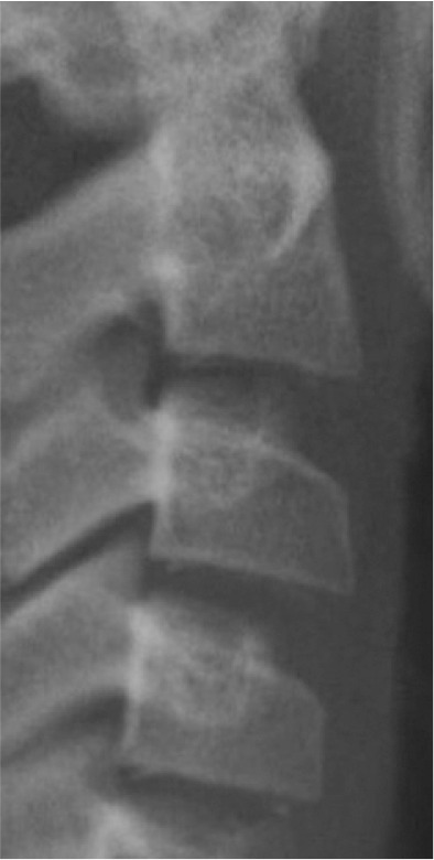
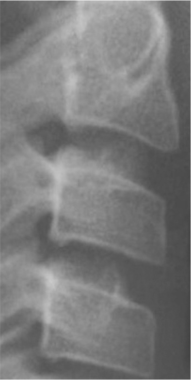
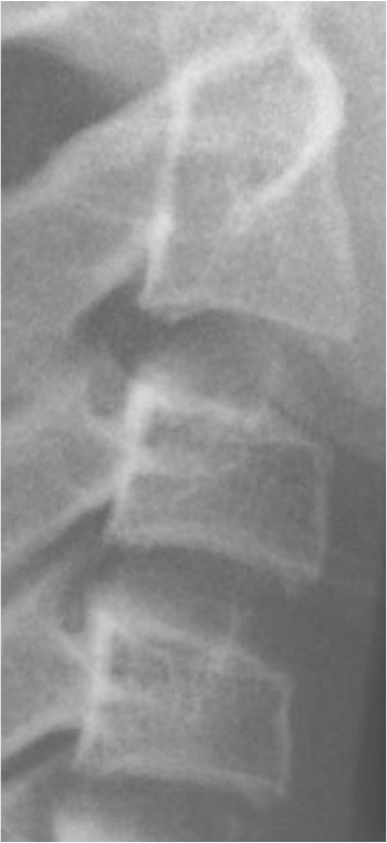
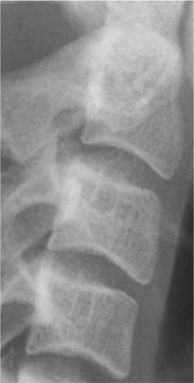
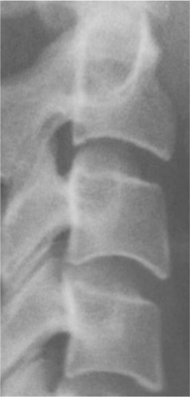
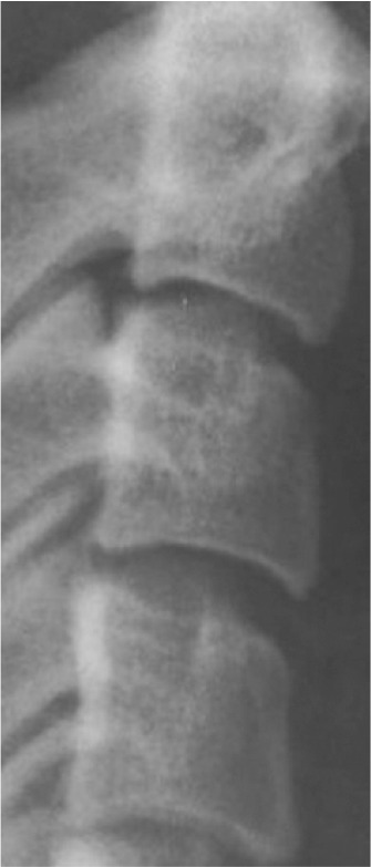
Classification of vertebral maturation degree was based on the guide proposed by McNamara and Franchi.³ The approach used in this study is briefly presented in Table 1. Using this approach, samples were divided into six cervical stage (CS) classes from CS1 to CS6 (Model A). Furthermore, the images were classified according to the CVM degrees based on the growth spurt (Model B), which was as follows:

Table 1.

Characteristics of various classes of cervical maturation degree

Stages		CS1	CS2	CS3	CS4	CS5	CS6
Inferior border concavity*	Vertebra
	C2	Absent	Present	Present	Present	Present	Present
	C3	Absent	Absent	Present	Present	Present	Present
	C4	Absent	Absent	Absent	Present	Present	Present
Body form†	C3	Trapezoid	Trapezoid	Trapezoid orHorizontal-rhomboid	Horizontal-rhomboid	Square‡ orHorizontal-rhomboid	Vertical-rhomboidor Square‡
	C4	Trapezoid	Trapezoid	Trapezoid orHorizontal-rhomboid	Horizontal-rhomboid	Square‡ orHorizontal-rhomboid	Vertical-rhomboidor Square‡

CS, cervical stage.

*Inferior border concavity is assessed by measuring the distance between the central point of the concavity and the line drawn from the outer endpoint of the inferior border, which is tangent to the most inferior point of the inferior border. A concavity characterizes a concave inferior border in the middle of the inferior vertebral border that is at least 7% of the length of the line connecting the two endpoints of the inferior border with an error range of 0.2% (based on the measurements conducted on the radiographic samples presented by McNamara et al.³).

^†In stages CS3, CS5, and CS6, the morphology of at least one of the vertebrae, either C3 or C4, must be characteristic (the bolded body form).

^‡A square morphology is characterized by equal length and width with an error range of 10%. The vertebra’s length is assessed by measuring the distance between the middle point of the superior border and the middle point of the line connecting the two end points of the inferior border. The width of the vertebra is assessed by measuring the distance between the middle points of the lateral borders.

1. Pre-pubertal: Including CS1 and CS2 (Class I),

2. Growth spurt: Including CS3 and CS4 (Class II), and

3. Post-pubertal: Including CS5 and CS6 (Class III).

Annotation was performed using cropped images and before preprocessing to avoid any possible biases. All radiographic images were classified independently by two orthodontists. Before the labeling procedure, a calibration session using 50 cephalograms was conducted for these orthodontists in order to ensure they reached a consensus on image classifications. In case of any disagreements, the final decision was made through agreement.

Data partitions

Finally, 890 images were divided randomly into the training, validation, and test sets. The number of samples in each class and each set is presented in Table 2. There were no overlaps between these sets.

Table 2.

Distribution of samples in the various classes

Data splitting set	CS1	CS2	CS3	CS4	CS5	CS6	Total
Training set	43	81	71	143	228	126	692
Validation set	5	10	6	25	35	18	99
Test set	5	10	6	25	35	18	99
Total	53	101	83	193	298	162	890
New augmentated samples in training set	641	603	613	541	456	558	3,412
Training set + oversampling + augmentation	684	684	684	684	684	684	4,104

CS, cervical stage.

The samples of classes with a lower number of images in the training set were oversampled to 228 images per category to solve the class imbalance challenge. Then data were augmented to increase the number of samples three times. The augmentation techniques were as follows:

1. Random crop (with the size of 60 × 100 pixels),

2. Random color jitter (e.g., random changes in brightness, contrast, saturation, and hue),

3. Random affine (e.g., random rotation [in the range of –20 to +20 degree], translating, and scaling [in the range of 0.8 to 1.1]), and

4. Random Gaussian noise.

All the augmentations applied with the probability of 0.5 only on the training samples. Before feeding the model, zero-padding was performed to change the input image’s size to 224 × 224 pixels.

Model architecture

In this section, we tried to evaluate the performance of various transfer learning models, all of which were pretrained on the ImageNet dataset, including ResNet-18, ResNet-50, ResNet-101, ResNet-152, VGG19, DenseNet, ResNeXt-50, ResNeXt-101, MobileNetV2, and InceptionV3.

To implement the deep learning model, the Python programming language and PyTorch library were used. In all the models, all the convolutional layers were frozen. However, the batch normalization layers were kept trainable because our dataset samples were very different from the ImageNet samples. However, one or two layers of trainable, fully connected layers were added to the output of the convolutional layers. The cross-entropy loss function was used as the objective loss in the last layer.

Training details

The training procedure was performed on a GeForce GTX 1050 graphic processor unit (Nvidia Corporation, Santa Clara, CA, USA). For each labeling approach (six-class and three-class), the models were trained separately. All the models were trained for 50 epochs. Training was performed using cross-entropy loss as the loss function. To further avoid overfitting, the early stopping strategy was used, in which the best model weights based on their performance (accuracy) on the validation set were saved. The grid search strategy was used for hyperparameter tuning of batch size, learning rate, and the optimizer.

Evaluation

We used the test set to evaluate our model performance on unseen data. Classification accuracy of all the trained models were presented. Details of the performance of the best-trained model based on the test set were also presented. Precision, recall, and F1-score of each class and each set based on the best model were also presented. These metrics are defined as follows:

$$\mathit{\text{classification Accuracy}}=\frac{TP+TN}{\#\mathit{\text{All Samples}}}$$

$$\mathit{\text{Precision}}=\frac{TP}{TP+FP}$$

$$\mathit{\text{Recall}}=\frac{TP}{TP+FN}$$

$$F1-\mathit{\text{score}}=\frac{2*\mathit{\text{Precision}}*\mathit{\text{Recall}}}{\mathit{\text{Precision}}\mathit{\text{Recall}}}$$

Where TP, TN, FP, and FN are the number of true-positive, true-negative, false-positive, and false-negative samples, respectively. The confusion matrices of the training, validation, and test sets were also presented.

In the final step, the test set of cephalograms was coded randomly and provided to two new orthodontists (N.M. and E.B.). Thereafter, the diagnoses of the AI model and orthodontists were compared to each other.

Statistical analysis

To compare AI diagnosis with that of human observers, weighted kappa and Cohen’s kappa statistical analyses were performed using SPSS for Windows, Version 15.0 (SPSS Inc., Chicago, IL, USA). The results of the weighted kappa and Cohen’s kappa analyses were interpreted as follows: kappa less than 0.2 indicated a slight agreement; kappa between 0.21 to 0.4 indicated a fair agreement; kappa between 0.41 to 0.6 indicated a moderate-to-fair agreement; kappa between 0.61 to 0.8 indicated a substantial agreement; and kappa more than 0.81 indicated an almost perfect agreement.¹⁹ Furthermore, interobserver percentage agreements were calculated as the number of agreements divided by the total number.

RESULTS

Data

The included data showed severe imbalance. As presented in Table 2, the lowest sample size was for CS1 (53; 5.96%), and the highest was for CS5 (298; 33.48%).

Model performance

The classification accuracy of all the trained models is presented in Table 3. ResNet-101 showed the best performance on the test set for both the six-class and three-class classifications. Following hyperparameter tuning, the batch size and learning rate were set to 4 and 0.001, respectively. Moreover, the Adam optimizer with a weight decay of 0.0001 was selected as the model optimizer.

Table 3.

Classification accuracy of various trained models on the validation and test sets

Trained model	Six-class			Three-class
	Validation set accuracy	Test set accuracy		Validation set accuracy	Test set accuracy
ResNet-101	62.63	61.62		75.76	82.83
ResNet-18	54.55	44.44		82.83	64.65
ResNet-50	65.66	50.51		82.83	79.8
VGG19	63.64	59.6		82.83	79.8
DenseNet	64.65	59.6		82.83	78.79
ResNeXt-50	65.66	55.56		82.83	65.66
ResNeXt-101	68.69	52.53		83.84	74.75
MobileNetV2	65.66	48.49		83.84	78.79
InceptionV3	54.55	51.52		77.78	69.7
ResNet-152	62.63	45.45		77.78	70.71

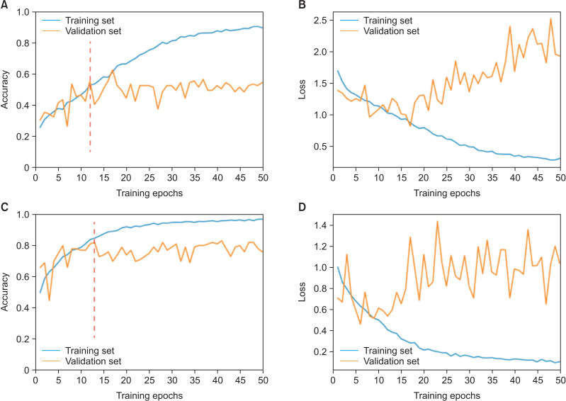
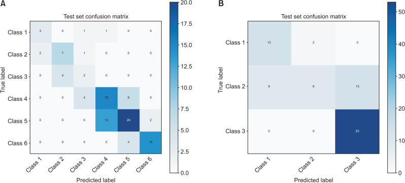
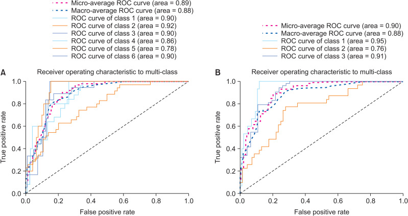
The accuracy and loss of 50 epochs of both the ResNet-101 model training processes are presented in Figure 1. As previously mentioned, we saved the models on the basis of their performance on the validation set. Regarding the six-class CVM diagnosis, the model’s validation and test accuracy were 62.63% and 61.62%, respectively. However, in the three-class classification, the model’s validation and test accuracy were 75.76% and 82.83%, respectively. The confusion matrix and receiver operating characteristic (ROC) curve of various classes in the test set are presented in Figures 2 and 3. Moreover, the precision, recall, and F1-score of each class in the training, validation, and test sets are reported in Table 4.

Figure 1.

Fifty epochs of ResNet-101 training. A, Changes in accuracy during training in both the validation and training sets in the six-class classification. B, Changes in loss during training in both the validation and training sets in the six-class classification. C, Changes in accuracy during training in both the validation and training sets in the three-class classification. D, Changes in loss during training in both the validation and training sets in the three-class classification. The epochs used for the early stopping strategy (to avoid overfitting) are shown as red dotted lines.

Figure 2.

A, Confusion matrix of the test set in the six-class classification of ResNet-101. B, Confusion matrix of the test set in the three-class classification of ResNet-101.

Figure 3.

A, Receiver operating characteristic (ROC) curve and the area under the ROC curve (AUC) score in the test set in the six-class classification of ResNet-101. B, ROC curve and the AUC score in the test set in the three-class classification of ResNet-101.

Table 4.

Precision, recall, and F1-score of the ResNet-101 model in the training, validation, and test sets in both the six-class and three-class classifications

Classification	Class	Training set				Validation set				Test set
		Precision	Recall	F1-score		Precision	Recall	F1-score		Precision	Recall	F1-score
Six-class	CS1	0.84	0.72	0.78		0.60	0.60	0.60		0.60	0.60	0.60
	CS2	0.52	0.58	0.55		0.55	0.60	0.57		0.64	0.70	0.67
	CS3	0.64	0.61	0.62		0.50	0.67	0.57		0.25	0.33	0.29
	CS4	0.75	0.80	0.77		0.67	0.72	0.69		0.52	0.60	0.56
	CS5	0.69	0.71	0.70		0.65	0.57	0.61		0.67	0.57	0.61
	CS6	0.83	0.81	0.82		0.65	0.61	0.63		0.88	0.78	0.82
Three-class	Class I	0.97	0.95	0.99		0.78	0.93	0.85		0.59	0.87	0.70
	Class II	0.90	0.87	0.94		0.82	0.58	0.68		0.82	0.29	0.43
	Class III	0.94	0.99	0.88		0.85	0.94	0.89		0.80	1.0	0.89

CS, cervical stage.

Model A performed the best in detecting CS6 with F1-scores of 0.82 and 0.63 on the test and validation sets, respectively. However, among the classes, the area under the ROC curve (AUC) score for CS2 was the best (AUC = 0.92). On the other hand, Model A showed the least accuracy in detecting the CS3 class. Model B had an F1-score of 0.89 on both the validation and test sets and was the best at detecting Class III.

Intraobserver agreement

The results regarding the intraobserver agreement are summarized in Table 5. The intraobserver agreements between the two orthodontists as well as that between the orthodontist N.M. and the AI models were classified as being substantial on the basis of weighted kappa and the abovementioned criteria.

Table 5.

Intraobserver agreement between the artificial intelligence (AI) model and two orthodontists (E.B. and N.M.)

Observer	Six-class CVM classification		Three-class CVM classification
E.B. & N.M.	Kappa	0.50	Kappa	0.59
	Weighted-kappa	0.70	Weighted-kappa	0.66
	Percentage agreement	60.60%	Percentage agreement	73.73%
AI & N.M.	Kappa	0.40	Kappa	0.47
	Weighted-kappa	0.65	Weighted-kappa	0.61
	Percentage agreement	53.53%	Percentage agreement	68.68%
AI & E.B.	Kappa	0.34	Kappa	0.40
	Weighted-kappa	0.59	Weighted-kappa	0.53
	Percentage agreement	48.48%	Percentage agreement	59.59%

CVM, cervical vertebral maturation.

DISCUSSION

The evaluation of CVM on lateral cephalograms is a common procedure used in orthodontic treatment for determining the optimal treatment initiation time. However, the nature of CVM analysis is subjective; moreover, it yields low reproducibility and is highly associated with the practitioner’s experience.^6,7 Studies have shown that using AI will lead to more accurate and reliable diagnoses.²⁰ The present study aimed to propose a deep learning model for skeletal maturation classification.

The challenge in conventional CVM stage evaluation is its poor reproducibility.⁷ Since the changes in stages are gradual, accurate classification of some CVM stages is difficult.²¹ Zhao et al.⁶ reported 40.7% to 79.1% interobserver agreement with weighted kappa values of 0.53 to 0.86. The interobserver agreement reported in this study was also in this range (60.60% agreement with a weighted kappa value of 0.70).

In this study, other than the six-class CVM degree approach, a new approach was applied that divides patients into three classes. In this approach, the six classes of CVM were further divided into three classes, each comprising two CVM classes. The justification for this approach is that one of the main applications of CVM classification is determining the optimal treatment timing for mandibular deficiencies. Therefore, on this basis, CS1 and CS2 present slow growth, CS3 and CS4 present increased growth velocity, and CS5 and CS6 present almost no substantial growth of the craniofacial region.²¹ Moreover, CS3 and CS4 can be considered as representing the optimal period for the treatment of skeletal Class II malocclusion.¹ When using this three-class approach, the interobserver agreement increased to 73.73%. Moreover, the model’s classification accuracy increased from 61.62% to 82.83% on unseen data.

The model reached an average classification accuracy of 61.62% in CVM degree classification using a transfer learning model. The best and worst performances were observed for CS6 and CS3, respectively. Moreover, the model showed an average classification accuracy of 82.83% in detecting pubertal stages. A few studies used artificial neural network models for CVM degree classification.^8,10,16 Amasya et al.¹⁰ obtained better classification accuracy (86.93%) than that of the current study, but they fed their models features extracted from manually identified landmarks. Although low-level features improved the classification, their approach still required manual marking of landmarks by a human, which is time-consuming and error-prone.²² However, as an advantage of the present study, only images were used as model inputs. Compared to a study by Kök et al.,¹⁶ who also used manually identified features, our model showed better performance in classifying CS4, CS5, and CS6. The weaker performance of other classes in our study is probably due to the lower number of samples in the training set, which considering data augmentation and oversampling, the model still overfitted on the training set.

Another study by Amasya et al.²³ assessed interobserver agreement between their previously developed model¹⁰ and human observers. That study reported an average interobserver agreement of 58.3% among the model and practitioners. However, the result of this study demonstrated an agreement of 51.01% between orthodontists and the model. The reason for the lower agreement in this study can be justified by the difference in the nature of the models; while our model was fed raw images, Amasya et al.²³ used handcrafted features.

The approach used in the present study is named “transfer learning,” which has been widely used in medical imaging.²⁴ In transfer learning, model knowledge, which has been gained by training on huge datasets, can be transferred for use on a new task. It is useful in medical imaging studies where a large amount of labeled medical data is inaccessible.¹⁵

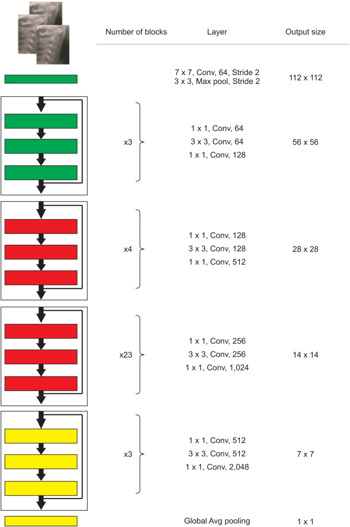
A fine-tuned ResNet pretrained on the ImageNet dataset architecture was used in this study. ResNet was introduced as a residual learning framework by He et al.²⁵ in 2015. This network can be used in specific tasks such as classification, segmentation, and object detection. The authors claimed that adding stack layers does not lead to better performance because of vanishing gradients. In contrast, to identify complex patterns, the network needs to be deeper. This problem has been solved by adding skip connections, and the skipped connections perform identity mapping. The network can be optimized easier with lower complexity than a plain network. The architecture shown in Figure 4 is a ResNet consisting of several residual blocks, and each block is made by convolution and batch normalization layers followed by the rectified linear unit activation function. Successful applications of pretrained ResNet have been widely reported in medical imaging tasks.²⁶

Figure 4.

The structure of ResNet-101.

Conv, convolution; Avg, average.

Data imbalance, which is defined as a skewed distribution in a study’s classes, is a common phenomenon in medical data.²⁷ An imbalanced dataset was one of the challenges faced in this study as there were only 43 samples in CS1, but there were 228 samples in CS5. Different techniques were employed, including oversampling and data augmentation, to overcome this challenge. The problem with imbalanced data in deep learning is that owing to the increased prior probability of classes with more samples, the samples of minority groups will be misclassified more often.²⁸ Oversampling minority groups and undersampling majority groups is a common approach used to overcome this challenge at the data level.²⁹

One of the main shortcomings of this study is that cropped images of ROIs were used for the classification. Future works should try to propose an end-to-end framework. This can be achieved through a two-stage network that detects ROIs and then classifies samples. The other approach can be the classification of whole cephalograms using a single model. The classification accuracy of the model can be increased by feeding more labeled data. Furthermore, few-shot image classification approaches, which require only a few examples of each class, may help further improve the performance of such models.

CONCLUSION

In the current study, an AI model was developed, and it had fair accuracy in detecting the CVM stages and desirable accuracy in detecting the pubertal stages. Feeding more labeled data and using state-of-the-art approaches may enhance the model’s performance. Nevertheless, the current model still needs improvement to enable its use in the clinical settings. Given the ongoing enhancement in data quality, we believe that AI will provide efficient assistance to practicing dentists in the future.

References

- 1.Baccetti T, Franchi L, McNamara JA., Jr The cervical vertebral maturation (CVM) method for the assessment of optimal treatment timing in dentofacial orthopedics. Semin Orthod. 2005;11:119–29. doi: 10.1053/j.sodo.2005.04.005. [DOI] [Google Scholar]
- 2.Hunter CJ. The correlation of facial growth with body height and skeletal maturation at adolescence. Angle Orthod. 1966;36:44–54. doi: 10.1043/0003-3219(1966)036<0044:TCOFGW>2.0.CO;2. [DOI] [PubMed] [Google Scholar]
- 3.McNamara JA, Jr, Franchi L. The cervical vertebral maturation method: a user's guide. Angle Orthod. 2018;88:133–43. doi: 10.2319/111517-787.1. [DOI] [PMC free article] [PubMed] [Google Scholar]
- 4.Franchi L, Baccetti T, De Toffol L, Polimeni A, Cozza P. Phases of the dentition for the assessment of skeletal maturity: a diagnostic performance study. Am J Orthod Dentofacial Orthop. 2008;133:395–400. quiz 476.e1–2. doi: 10.1016/j.ajodo.2006.02.040. [DOI] [PubMed] [Google Scholar]
- 5.Flores-Mir C, Nebbe B, Major PW. Use of skeletal maturation based on hand-wrist radiographic analysis as a predictor of facial growth: a systematic review. Angle Orthod. 2004;74:118–24. doi: 10.1043/0003-3219(2004)074<0118:UOSMBO>2.0.CO;2. [DOI] [PubMed] [Google Scholar]
- 6.Zhao XG, Lin J, Jiang JH, Wang Q, Ng SH. Validity and reliability of a method for assessment of cervical vertebral maturation. Angle Orthod. 2012;82:229–34. doi: 10.2319/051511-333.1. [DOI] [PMC free article] [PubMed] [Google Scholar]
- 7.Nestman TS, Marshall SD, Qian F, Holton N, Franciscus RG, Southard TE. Cervical vertebrae maturation method morphologic criteria: poor reproducibility. Am J Orthod Dentofacial Orthop. 2011;140:182–8. doi: 10.1016/j.ajodo.2011.04.013. [DOI] [PubMed] [Google Scholar]
- 8.Makaremi M, Lacaule C, Mohammad-Djafari A. Deep learning and artificial intelligence for the determination of the cervical vertebra maturation degree from lateral radiography. Entropy. 2019;21:1222. doi: 10.3390/e21121222. [DOI] [Google Scholar]
- 9.Khanagar SB, Al-Ehaideb A, Maganur PC, Vishwanathaiah S, Patil S, Baeshen HA, et al. Developments, application, and performance of artificial intelligence in dentistry - a systematic review. J Dent Sci. 2021;16:508–22. doi: 10.1016/j.jds.2020.06.019. [DOI] [PMC free article] [PubMed] [Google Scholar]
- 10.Amasya H, Yildirim D, Aydogan T, Kemaloglu N, Orhan K. Cervical vertebral maturation assessment on lateral cephalometric radiographs using artificial intelligence: comparison of machine learning classifier models. Dentomaxillofac Radiol. 2020;49:20190441. doi: 10.1259/dmfr.20190441. [DOI] [PMC free article] [PubMed] [Google Scholar]
- 11.LeCun Y, Bengio Y, Hinton G. Deep learning. Nature. 2015;521:436–44. doi: 10.1038/nature14539. [DOI] [PubMed] [Google Scholar]
- 12.Schwendicke F, Samek W, Krois J. Artificial intelligence in dentistry: chances and challenges. J Dent Res. 2020;99:769–74. doi: 10.1177/0022034520915714. [DOI] [PMC free article] [PubMed] [Google Scholar]
- 13.Mohammad-Rahimi H, Nadimi M, Ghalyanchi-Langeroudi A, Taheri M, Ghafouri-Fard S. Application of machine learning in diagnosis of COVID-19 through X-ray and CT images: a scoping review. Front Cardiovasc Med. 2021;8:638011. doi: 10.3389/fcvm.2021.638011.3d26d1f99b334befa87fe1bafca467c0 [DOI] [PMC free article] [PubMed] [Google Scholar]
- 14.Mohammad-Rahimi H, Nadimi M, Rohban MH, Shamsoddin E, Lee VY, Motamedian SR. Machine learning and orthodontics, current trends and the future opportunities: a scoping review. Am J Orthod Dentofacial Orthop. 2021;160:170–92.e4. doi: 10.1016/j.ajodo.2021.02.013. [DOI] [PubMed] [Google Scholar]
- 15.Ravishankar H, Sudhakar P, Venkataramani R, Thiruvenkadam S, Annangi P, Babu N, et al. Understanding the mechanisms of deep transfer learning for medical images. Springer International Publishing; Cham: 2016. pp. 188–96. [DOI] [Google Scholar]
- 16.Kök H, Acilar AM, İzgi MS. Usage and comparison of artificial intelligence algorithms for determination of growth and development by cervical vertebrae stages in orthodontics. Prog Orthod. 2019;20:41. doi: 10.1186/s40510-019-0295-8.9e00597c2a594eeeac0d562615036f6b [DOI] [PMC free article] [PubMed] [Google Scholar]
- 17.Mongan J, Moy L, Kahn CE., Jr Checklist for Artificial Intelligence in Medical Imaging (CLAIM): a guide for authors and reviewers. Radiol Artif Intell. 2020;2:e200029. doi: 10.1148/ryai.2020200029. [DOI] [PMC free article] [PubMed] [Google Scholar]
- 18.Wang CW, Huang CT, Lee JH, Li CH, Chang SW, Siao MJ, et al. A benchmark for comparison of dental radiography analysis algorithms. Med Image Anal. 2016;31:63–76. doi: 10.1016/j.media.2016.02.004. [DOI] [PubMed] [Google Scholar]
- 19.Landis JR, Koch GG. The measurement of observer agreement for categorical data. Biometrics. 1977;33:159–74. doi: 10.2307/2529310. [DOI] [PubMed] [Google Scholar]
- 20.Tajmir SH, Lee H, Shailam R, Gale HI, Nguyen JC, Westra SJ, et al. Artificial intelligence-assisted interpretation of bone age radiographs improves accuracy and decreases variability. Skeletal Radiol. 2019;48:275–83. doi: 10.1007/s00256-018-3033-2. [DOI] [PubMed] [Google Scholar]
- 21.Graber LW, Vanarsdall RL, Jr, Vig KWL, Huang GJ. Orthodontics: current principles and techniques. 6th ed. Elsevier; St. Louis: 2016. [Google Scholar]
- 22.Yu HJ, Cho SR, Kim MJ, Kim WH, Kim JW, Choi J. Automated skeletal classification with lateral cephalometry based on artificial intelligence. J Dent Res. 2020;99:249–56. doi: 10.1177/0022034520901715. [DOI] [PubMed] [Google Scholar]
- 23.Amasya H, Cesur E, Yıldırım D, Orhan K. Validation of cervical vertebral maturation stages: artificial intelligence vs human observer visual analysis. Am J Orthod Dentofacial Orthop. 2020;158:e173–9. doi: 10.1016/j.ajodo.2020.08.014. [DOI] [PubMed] [Google Scholar]
- 24.Yu Y, Lin H, Meng J, Wei X, Guo H, Zhao Z. Deep transfer learning for modality classification of medical images. Information. 2017;8:91. doi: 10.3390/info8030091. [DOI] [Google Scholar]
- 25.He K, Zhang X, Ren S, Sun J. Deep residual learning for image recognition. Paper presented at: 2016 IEEE Conference on Computer Vision and Pattern Recognition; 2016 Jun 27-30; Las Vegas, USA. Piscataway: Institute of Electrical and Electronics Engineers; 2016. pp. 770–8. [DOI] [Google Scholar]
- 26.Wang W, Liang D, Chen Q, Iwamoto Y, Han XH, Zhang Q, et al. Medical image classification using deep learning. In: Chen YW, Jain LC, editors. Deep learning in healthcare: paradigms and applications. Springer; Cham: 2020. pp. 33–51. [DOI] [Google Scholar]
- 27.Shin HC, Tenenholtz NA, Rogers JK, Schwarz CG, Senjem ML, Gunter JL, et al. Medical image synthesis for data augmentation and anonymization using generative adversarial networks. Springer International Publishing; Cham: 2018. pp. 1–11. [DOI] [Google Scholar]
- 28.Johnson JM, Khoshgoftaar TM. Survey on deep learning with class imbalance. J Big Data. 2019;6:27. doi: 10.1186/s40537-019-0192-5.d7c13b2130ee4ee68add6580cabd608c [DOI] [Google Scholar]
- 29.Ramentol E, Caballero Y, Bello R, Herrera F. SMOTE-RSB*: a hybrid preprocessing approach based on oversampling and undersampling for high imbalanced data-sets using SMOTE and rough sets theory. Knowl Inf Syst. 2012;33:245–65. doi: 10.1007/s10115-011-0465-6. [DOI] [Google Scholar]