Spectral Wavelet-feature Analysis and Classification Assisted Denoising (SWANCAD) for Enhancing Magnetic Resonance Spectroscopy

Abstract

Magnetic resonance spectroscopy (MRS) is capable of revealing important biochemical and metabolic information of tissues non-invasively. However, the low concentrations of metabolites often lead to poor signal-to-noise ratio (SNR) and long acquisition time. Therefore, applications of MRS in detection and quantitative measurements of metabolites in vivo remain to be limited. Reducing or even eliminating noise can improve SNR sufficiently to obtain high quality spectra in addition to increasing the number of signal averaging (NSA) or the field strength, both of which are limited in clinical applications. We present a Spectral Wavelet-feature Analysis and Classification Assisted Denoising (SWANCAD) approach to differentiate signal and noise peaks in magnetic resonance spectra based on their respective wavelet features, followed by removing the identified noise components to improve SNR. The performance of this new denosing approach was evaluated by measuring and comparing SNRs and quantified metabolite levels of the low NSA spectra (e.g., NSA = 8) before and after denoising using the SWANCAD approach or conventional spectral fitting and denoising methods, such as LCModel and wavelet threshold methods as well as the high NSA spectra (e.g., NSA = 192) recorded in the same sampling volumes. The results demonstrated that SWANCAD offers a more effective way to detect the signals and improve SNR by removing noise from the noisy spectra collected with low NSA or in the sub-minute scan time (e.g., NSA = 8 or 16 seconds). The potential applications of SWANCAD include using low NSA to accelerate MRS acquisition while maintaining adequate spectroscopic information for detection and quantification of the metabolites of interest when a limited time is available for an MRS exam in the clinical setting.

1. Introduction

Magnetic resonance spectroscopy (MRS) is one of the few non-invasive imaging tools capable of revealing biochemical and metabolic processes of tissue in vivo by directly detecting and measuring concentrations of biochemical substances and metabolites¹. Since MRS detectable endogenous chemicals are typically at the concentration range of millimolar levels or slightly higher, MRS signal is orders of magnitude lower than the signal of water, which is the source of signal in conventional magnetic resonance imaging (MRI). To overcome the intrinsic limitation of low signal-to-noise ratio (SNR) of MRS, data acquisition is performed using large sample volumes and a high number of signal averages (NSA), in which both signal and noise are summed over repeated acquisitions and subsequently averaged². However, both of these options have inevitable limitations; while the former causes low spatial resolution and loss of specificity when sampling the heterogeneous tissue, the latter leads to long data acquisition time and spectral artifacts from time-varying signal contaminations, such as patient motion and field drift. The inherent low sensitivity along with long acquisition time are the major impeding factors in integrating MRS into clinical applications, even though the metabolic changes and metabolite biomarkers have been increasingly recognized as critical diagnostic information in individualized medicine³.

The efforts to accelerate MRS includes the development of ultrafast acquisition methods⁴ to obtain high-resolution MRSI, utilization of ultra-high field system or parallel data acquisition, and implementation of data-driven reconstructions⁵. On the other hand, one of the strategies to improve the sensitivity of MRS with existing instrumentation capabilities at the current clinical field strength (i.e., 3T) is to improve SNR by reducing the noise level or even completely removing noise while retaining the signal as part of the post-processing step. While the noise can be mitigated by applying a smoothing filter, such as Gaussian filter, in either spatial or spectral domains, filtering causes loss of a portion of the signal as it is impossible to completely differentiate noise from the signal⁶. Furthermore filtering also leads to spectral linewidth broadening, therefore compromising spatial resolution⁷. It should be noted that a smoothing filter assumes that the distribution of the random noise has a mean of zero; this assumption fails, however, in the acquisition scenario of using phased array coils with a non-uniform noise distribution⁸. Other denoising approaches that have been investigated include: the wavelet thresholding method which separates signal and noise wavelets based on a preset threshold value^9–13 and the wavelet shrinkage method which uses specific wavelet coefficients to distinguish the signal from the noise¹⁴.

The wavelet based denoising algorithms have been shown to retain the spectral line shape across the spectral domain of mass spectroscopy data¹⁵ or MRS data¹⁶. Specifically, a spectrum can be decomposed to its wavelet components; these components can subsequently be used to differentiate signals and noise. By treating signal peaks as low rank subspace raw data¹⁶, singular value decomposition and principal component analysis can be applied to find wavelet components representing the signals. Using the data-driven low rank component analysis approach to minimize the approximation error within the subspace of spectroscopic data can improve SNR and spectral quality, regardless of the frequency content of a signal and discontinuities of the shrinkage function¹⁷. The simple wavelet shrinkage can minimize the empirical wavelet coefficients towards zero, thereby removing noise from the input spectra¹⁸. In addition, the signal peaks from a given metabolite should appear at the distinctive frequencies or chemical shifts, which provide frequency features of each metabolite based on its unique chemical structure. Furthermore, it is conceivable that signals and noise in the spectrum should have different types of wavelet shapes. Therefore, they can be differentiated based on the characteristics or features of their spectral segments identified by the wavelet transformation process. Thus, identification of spectral wavelet features should enable machine or deep learning-based approaches for enhancing the SNR of MRS data.

In this work, we present a data-driven Spectral Wavelet-feature Analysis and Classification Assisted Denoising (SWANCAD) method for characterizing and differentiating signal and noise peaks in MRS data and subsequently removing noise without compromising the signal peaks to obtain high SNR spectra. Source wavelets which are the waveforms with specific shapes or patterns found in the library of wavelets in the literature were used to scan across the spectral domain using continuous wavelet transform (CWT) to identify and extract specific characteristics of wavelet presentations for each signal and noise, henceforth referred to as spectral wavelets. To improve the accuracy of the spectral wavelet classification, 29 features characterizing these wavelets were selected and then fed into a support vector machine (SVM)¹⁹ to classify the signal and noise peaks of MRS data. We demonstrate that the SWANCAD approach can effectively reduce the noise level of low NSA spectra collected in the short acquisition time of 16 seconds, obtaining comparable metabolite signals to those from long scans, e.g., ~6-7 minutes used as an example in this work. We further demonstrated the potential clinical application of this approach to retain and recover diagnostic information from low SNR data from patients.

2. Method

2.1. Theory

Wavelets are particularly suitable for isolating abrupt changes in signal. A wavelet is a function $\phi (t)$ in $\mathcal{L}$ ²(R) such that $\phi (t)$ satisfies the following equation (Eq. 1)^20,21:

$${\int }_{-\infty }^{+\infty }\phi (t)dt=0$$ Eq. 1

Compared to the discrete wavelet transform previously used by others for denoising Raman spectra²², CWT is capable of detecting local changes in a spectrum. The basic CWT is a step by step process, starting with selecting source wavelets from a library of different wavelets based on its resemblances to the signal and noise patterns of the spectrum. The selected source wavelets are then used to compare each part of the original spectrum, respectively, by calculating the correlation coefficient between each source wavelet representing signal or noise and the pairing part of the spectrum. Subsequently, each source wavelet is shifted to the next part of the spectrum until covering the entire spectral domain to find the spectral wavelets in the spectrum that have distinctive waveform characteristics that closely match the source wavelets determined by the analysis of correlations between the pairing source wavelets and parts of the spectrum (described in 2.6). These unique wavelets from each input spectrum, i.e., spectral wavelets, are used to characterize signal and noise in the spectroscopic data. The CWT operation is repeated iteratively with different source wavelets that describe signals or noise. Thus CWT described in Eq. 2 is an operation whereby the continuous shifting and scaling of source wavelets result in the calculation of wavelet coefficients, $X_{wt(\tau ,s)}$ which yields characteristics of upward and downward slopes of a signal peak^{23, 24}:

$$X_{wt(\tau ,s)}={\int }_{-\infty }^{+\infty }x(t){\phi }_{\tau ,s}(t)dt$$ Eq. 2

In Eq. 2, $x(t)$ is the input spectrum, while $\tau$ represents a shift away from or towards the source wavelet, s is the scale parameter that allows for shape manipulation of the source wavelet. While CWT, much like discrete WT, is a digital operation, the former uses a single sample shifting at each increment (i.e., $\tau =1$), whereas the latter often skips one or more samples with each shift step (i.e., $\tau \ge 2$); as such CWT results in a finer characterization of the correlation between the input signal and the wavelet. ${\phi }_{\tau ,s}\left(t\right)$ is described by Eq. 3.

$${\phi }_{\tau ,s}(t)=\frac{1}{\sqrt{\left|s\right|}}\phi \left(\frac{t-\tau }{s}\right)$$ Eq. 3

The resulting wavelet coefficients can be used to efficiently extract spectral features²⁵. Specifically, these coefficients contain characteristics of peaks and troughs that can be used to detect the position and amplitude of peaks in $x(t)$. In the current study, the CWT was applied to the data in the spectral domain using two source wavelets with 6 and 20 vanishing moments selected from Daubechies wavelets (db6 and db20)²⁶. Spectral wavelets were identified from each input spectrum, which were used to characterize signal and noise in the spectrum later. At a $s$ in ${\phi }_{\tau ,s}$, all peaks in $x\left(t\right)$ can be detected²⁷. The maximum number of spectral wavelets (N_m) needed to represent an input signal can be calculated with Eq. 4, using N, which is the number of data points across the entire spectrum and N_s, which corresponds to the number of selected source wavelets²⁸.

$$N_m=Round\left({\mathit{log}}_2\left(\frac{N}{N_s}-1\right)\right)$$ Eq. 4

After using the SVM classification algorithm to select spectral wavelets of signals, the inverse continuous wavelet transform was then applied to reconstruct the final denoised spectrum. Only the selected spectral wavelets of signals were used to reconstruct each denoised spectrum. The inverse continuous wavelet transform is expressed by Eq. 5 as:

$$x(t)={\int }_{-\infty }^{+\infty }{\int }_{-\infty }^{+\infty }{X}_{wt(\tau ,s)}\phi \left(\frac{t-\tau }{s}\right)d\tau \frac{ds}{s^2}$$ Eq. 5

To analyze the spectral data included in this study, the scale factor s was set at 1 while the source wavelet applied was shifted over each data point cross the spectral domain (e.g., 1024 data point).

2.2. MRS data from the brain phantom

A phantom (Model 2152220, GE Healthcare, Chicago, IL) containing selected brain metabolites with known concentrations, including N-acetylaspartate (NAA, 12.5 mM), creatine (Cre, 10 mM), choline (Cho, 3 mM), lactate (Lac, 15 mM), glutamate (Glu, 12.5 mM) and myo-inositol (MI, 7.5 mM) was placed in a 20-channel phase-array head coil positioned at the iso-center of a 3T MR scanner (MAGNETOM Prisma, Siemens Healthcare, Erlangen, Germany).

T₁-weighted magnetization-prepared rapid acquisition gradient echo (MPRAGE) images were first acquired using parameters of TR of 500 ms; TE of 8.7 ms; flip angle of 90°, matrix of 180×240 mm², field of view (FOV) of 192×256 pixels, slice thickness of 2 mm, to assist localization of the sampling voxel (20×20×20 mm³). The standard shimming method implemented on the scanner was applied. Chemical shift selected pre-saturation scheme was used for water suppression²⁹ in all MRS acquisitions. Single-voxel proton (¹H) spectroscopy (SVS) data were collected using a point resolved spectroscopy sequence (PRESS) with echo time (TE) of 30 ms, repetition time (TR) of 2000 ms, acquisition bandwidth of 1200 Hz and vector size of 1024.

SVS data acquisitions were performed on the phantom at different sampling locations, i.e., one voxel at the iso-center of the phantom followed by three additional locations, each (same volume) shifted 30 mm away from the initial iso-center position to the anterior, right, and feet direction, respectively. In each session, two spectral datasets with NSA of 192 (henceforth referred to as the high NSA spectra) and 8 (henceforth referred to as the low NSA spectra) were acquired at the same voxel locations and volumes. The data acquisition was repeated 5 times in separate scan sessions in order to generate sufficient training data for the classification algorithm of SVM, resulting in a total of 20 high NSA spectra and 20 low NSA spectra. For the low NSA data, each single acquisition was saved individually, allowing for processing the single acquisition spectra as well as the averaged result from each acquisition. The representative voxel locations and their corresponding spectra are shown in Figure 1. The total MRS acquisition times, excluding pre-acquisition shimming and water suppression, were 24 seconds for the low NSA spectra, including 4 preparation scans and 6 minutes and 40 seconds for the high NSA spectra, including 8 prescans. Phase cycling of 4 was used for both low and high NSA data acquisition.

Figure 1.

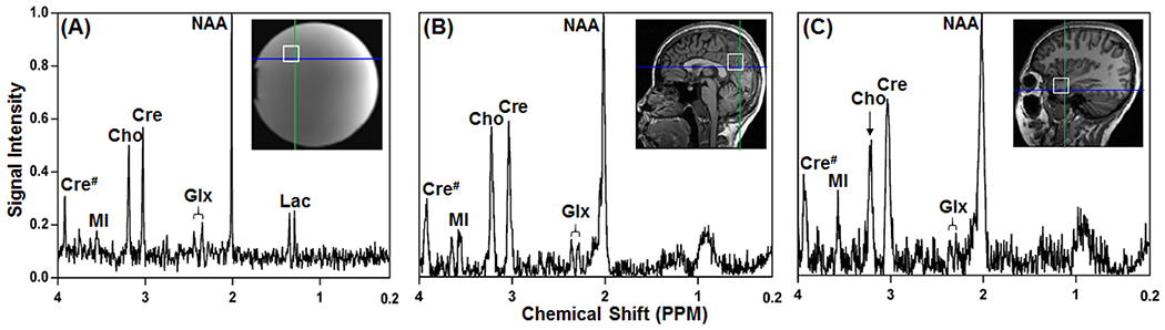
Examples of single voxel locations selected in a brain spectroscopy phantom (A), parietal (B) and temporal (C) regions of a healthy human brain and corresponding spectra acquired with NSA= 8. Peaks of NAA, Cre, Cho and Lac are found at chemical shifts of 2.02, 3.05, 3.22 and 1.33 ppm, respectively. Glx is composed of Glu and Gln which may partially overlap at the field strength of 3 Tesla. Abbreviations: Cho, choline; Cre and Cre^#, creatine; NAA, Nacetylaspartate; Lac, lactate; MI, myo-inositol; Glu, glutamate and Gln, glutamine; # indicates the methylene group (~3.95 ppm) from Cre. N-methyl group Cre appears at ~3.05 ppm.

To further characterize and test the proposed denoising classifier (described in detail in sections 2.6), a “noise-only” scan was performed at the iso-center voxel location as described above. For this experiment, the radiofrqunency (RF) power of the excitation pulse was turned off, leaving protons from metabolites and water in the phantom not excited. Therefore, recorded spectra contain only noise and possible signal contamination from the imperfect 180° refocusing pulse. The recorded noise-only data were subsequently pre-processed and denoised with the different methods.

2.3. MRS data from healthy volunteers

We collected brain SVS data from healthy subjects (N = 5, four females, age range: 29-41 years) with the same acquisition protocol used for the phantom scan. The voxels of 20 x 20 x 20 mm³ were selected in parietal and temporal regions as shown in Figure 1. Similar to data collection from the phantom, two spectral datasets, one high NSA spectrum (i.e., NSA of 192) and one low NSA spectrum (i.e., NSA of 8), were acquired from the same voxel under the same shimming and water suppression conditions. The human subject study was done in accordance with the institutional review board and written consents were obtained from all of participants.

2.4. MRS data from brain tumor patients

To demonstrate and evaluate the performance of the reported SWANCAD approach for a clinically relevant application, we retrospectively extracted several individual spectra from the multivoxel chemical shift imaging (CSI) data collected from four high grade glioblastoma patients (3 male and 1 female, age between 48 – 57 years old). The data collection on these patients was approved by the institutional review board with the written consents obtained from all these patients.

CSI, which is also called multi-voxel spectroscopic imaging of a selected region of interest (ROI), was performed on these patients using a stimulated-echo acquisition mode (STEAM) sequence on the same 3T MRI scanner with a 20-channel head coil array. A multi-slice T₂ weighted flow attenuated inversion recovery (FLAIR) sequence was used to reveal the tumors based on the hyperintense T₂ signals and anatomic structures of the brain. FLAIR imaging parameters included: TR of 9600 ms; TE of 93 ms; inversion time of 2566 ms; flip angle of 130°; FOV of 240 x 240 mm, matrix of 408 x 512 and slice thickness of 5 mm. FLAIR images were then used to place the ROI covering the tumor and the normal contralateral brain tissue for CSI data collection using the following parameters: TR/TE of 1800/68 ms, slice thickness of 20 mm, FOV of 140 x 140 mm with a matrix size of 8 x 8 interpolated to 16 x 16, which yielded each single voxel in the multi-voxel setting with a voxel size of 8.8 x 8.8 x 20 mm³. The total CSI acquisition time was approximately 7 minutes and 12 seconds with elliptical phase encoding and NSA of 8. Four spectra from individual voxels of each tumor, well within the T₂ enhanced tumor areas based on the overlaid FLAIR images, and four from the normal regions in the contralateral hemisphere were extracted from each CSI data for analysis with different post-processing methods. A total of 16 individual spectra from the tumor regions and 16 spectra from the normal regions of four patients were used.

2.5. Spectral preprocessing

The raw time domain free induction decay (FID) data were first converted to the frequency domain spectra after Fourier transformation using the function included in the program package of LCModel (version 6.3-1H)³⁰, a widely used MRS data processing software package. LCModel uses a spectral fitting approach based on templates of metabolites known in specific types of tissue or samples and frequency or chemical shift information to generate a spectrum with the signals matching those in the metabolite templates at the specific chemical shifts. After applying the phase correction using LCModel, spectral baseline correction was performed by fitting the spectrum with a sextic polynomial equation and subsequently subtracting it from the whole spectrum using an in-house program written in MATLAB (R2019a, The MathWorks Inc., Natick, MA) and the algorithm previously reported³¹. Finally each baseline-corrected spectrum was normalized over the entire spectral range for the subsequent analyses of denoising performances using NAA peak at the chemical shift of 2.02 ppm as the reference³².

2.6. Feature extraction and classification

The source wavelets from the Daubechies wavelet family were selected to seek wavelet features from high NSA MRS data. Daubechies wavelets have been used previously for denoising medical images, including MRI, ultrasound, x-ray, CT image³² and spectral data³³. For this proof-of-principal study, we used the Daubechies source wavelets with 6 and 20 vanishing moments, since they are representatives of the shapes of signal peaks, which are typically less oscillating, and noise peaks, which oscillate at higher frequencies³⁴. For each signal source wavelet, the length or window would cover 50 data points or a range of 0.24 ppm (50 x 0.0048 ppm = 0.24 ppm) based on the dataset collected in this study, while for the noise source wavelet, the length or window would cover 15 data points or a range of 0.072 pm (15 x 0.0048 ppm = 0.072 ppm). Using each source wavelet, the high NSA spectra were transformed into the wavelet space using the CWT to identify specific spectral wavelets representing metabolite signal or noise peaks in each spectrum based on their coefficients. Specifically, each selected source wavelet representing signals or noise, was used as the waveform window “scanning” through the input spectrum at one data point per step. The source wavelets were paired to each part of the spectrum and their match local maxima and local minima. Linear Pearson correlation was used to assess the fit of each source wavelet and each part of the spectrum using the first local minimum at the starting point and the last local minimum as the ending point. Statistically significant correlation (with p < 0.05 deemed significant) was used to determine the spectral wavelets which have the highest correlation coefficients (lowest p-values). Based on Eq. 4, 8 spectral wavelets with the highest correlation coefficients (lowest p-values) derived from two source wavelets were sufficient in describing the spectra acquired in this study for denoising. The spectral wavelets were obtained first from the input high NSA spectrum.

To characterize various types of spectral profiles, spectral wavelets are typically described with features, such as the magnitude or intensity of peak, chemical shift, the range of spectral peaks, skewness, maximum to minimum difference, entropy, wavelet energy, spectral centroids, spectral slope, peak to root-mean-square, and spectral flatness^35–37. In the current study, 29 features describing or measuring the properties of the spectral wavelets were used to classify signal and noise based on the ealier reports^35–37. A list of all 29 features can be found in Table 1. In order to identify the features with the most significant contribution to the accuracy of signal and noise classification, these 29 features extracted from signal and noise spectral wavelets were input into the SVM classification algorithm³⁸ implemented with a wrapped-forward approach³⁹. While any classifier could be optimized and tested for the SWANCAD approach, SVM classifier was chosen because of its superior performance in handling high dimensional data while being robust despite a relatively small set of training data¹⁸. We split our initial data of 16 high NSA spectra (i.e., 6 high NSA spectra collected from the phantom, 10 high NSA spectra collected from the parietal and temporal lobes of five healthy volunteers) into the training dataset (N = 15) and a testing dataset. The training set and testing set were randomly partitioned using leave-one-out approach⁴⁰ with a grid search⁴¹ to tune and select the parameters. This process was performed with 100 times repetition and then averaged 100 results to produce a single estimation of classification performance. Moreover we used the radial basis function (RBF) kernel and polynomial kernel functions in the configuration of the SVM classification to improve the performance of SVM classifier as demonstrated by others in earlier studies⁴². The contributions of each of the 29 spectral wavelet features were evaluated individually based on the resulting classification accuracy in differentiation of signal and noise. The spectral wavelets and the wavelet features resulting in the highest classification accuracy were extracted for subsequent denoising of the low NSA data.

Table 1.

Features in spectral wavelets of spectra derived from the training datasets

Feature	Name
F1	Chemical shift
F2	Area under the curve
F3	Full width at half maximum
F4	Amplitude
F5	Kurtosis
F6	Range of frequency fluctuation
F7	Skewness
F8	Square root of the amplitude
F9	Spectral slope
F10	Maximum-to-minimum difference
F11	Wavelet energy
F12	Root-mean-square
F13	Spectral flatness
F14	Spectral centroid
F15	Peak to Root-mean-square
F16	Entropy
F17	Spectroscopy envelope
F18	Mean spectral
F19	Standard of spectral
F20	Power bandwidth
F21	Total harmonic distortion
F22-F29	Mel-Frequency cepstral coefficient

2.7. Spectral denoising and performance evaluation

Signal-to-noise ratio was used as a metric to evaluate denoising performance of the trained SWANCAD algorithm. SNR was calculated as follows:

$$SNR=\frac{I}{\sigma }$$ Eq. 6

where I is the maximum intensity of selected metabolite peaks (e.g., NAA, Cho, Cre, MI, Lac, Glu or Glx) in the spectra and σ is the standard deviation of noise-only region of the spectra, measured from the last 100 points of the spectrum in the up-field region where there is no known metabolite peaks⁴³

For this proof-of-concept study, we only include brain metabolites well documented in the literature as they are clearly detected in the spectra and commonly used for clinical diagnosis. The baseline corrected spectra were used to calculate the SNRs of selected metabolites. The performance of the SWANCAD denoising approach was evaluated by comparing the SNRs of low NSA spectra (N = 10) processed by SWANCAD and two other commonly used MRS data post-processing methods; LCModel spectral fitting approach with the convolution range adjusted to obtain a more accurate line shape estimation⁴⁴ and the wavelet threshold denoising approach with updated semisoft threshold⁴⁵. In addition, the same metrics, i.e., SNR, were used to evaluate the denoising efficiency of the individual spectra extracted from CSI data collected from brain tumor patients.

Furthermore, we investigated whether denoising spectral data with different denoising approaches may affect the metabolite quantification. In this case, we used the data from the spectroscopic phantom and from the parietal region of healthy subjects, given the much less influence of the field inhomogeneity on the accuracy of metabolite quantification compared to the data collected from the temporal lobe. The quantification of the metabolites detected in the spectra was performed by calculating definite integrals of the selected peaks from the metabolites of interest (i.e., NAA, Cre, Cho, MI, Lac and combined Glu and Gln or (Glx) using an in-house Matlab program, as the integral of the peak in relation to the number of protons in the structure of the molecules is directly correlated to the metabolite concentration. Briefly, the local maximum and local minima were found first based on the signal intensity in the region of the selected peak using the first derivative test. The integration of the single signal peak then was performed following the curve between the two boundaries defined by the pair of local minima, assuming a unimodal distribution⁴⁶ in which the local maximum is located between two local minima. For integrating the metabolite signal with multiple local maxima, e.g., the doublet of Lac and Glx, a bimodal distribution was used⁴⁷. The integral can be approximated by using the trapezoidal rule, which works by approximating the region under the curve of the function as a trapezoid. Finally, the integrals calculated from the peaks of the methyl protons in the -CH₃ group of the selected metabolites are used as the measurement of metabolite levels. For the comparison of spectra processed using different methods, the concentrations calculated from the high NSA (NSA = 192) spectra (in the same sampling volume) was used without application of denoising. The results were averaged from multiple measurements of the same sampling volumes in the phantom (N = 3) or human parietal and lobes (N = 5). In addition, ratios of metabolites, i.e., integrals of methyl proton peaks of NAA, Cho, MI, and Lac divided by the integral of the methyl protons peak of Cre were obtained for comparison as well⁴⁸.

2.8. Statistical analysis

Statistical analyses are performed using the statistics toolbox included in MATLAB (R2019a, the MathWorks Inc., Natick, MA). The pairwise t-test was used to compare the SNR metric of original low NSA spectra from the phantom and corresponding denoised spectra for a total of 80 data. Denoised low NSA phantom spectra were also compared to the high NSA spectra collected in the same voxel. The SNR metric of human subject data were used to compare the denoised low NSA spectra and high NSA spectra (N = 10) using pairwise t-test. The comparison of the SNR improvement by SWANCAD, LCModel, and wavelet threshold denosing approaches was performed using one-way analysis of variance (one-way ANOVA) with Student Newman Keuls test using SPSS Statistics (version 24.0, IBM, Armonk, NY). The p-value (P < 0.05) was used to determine the statisitical significance of the difference in the comparison. One-way ANOVA with Student Newman Keuls test was also used to determine the differences in the metabolite ratios obtained from the spectra denoised with different algorithms and the spectrum collected with high NSA which serves as a reference for more accurate metabolite ratios due to its high SNR without any denoise influence.

3. Results

3.1. Signal and noise spectral wavelet feature extraction and classification

Eight spectral wavelets, as shown in Figure 2, were identified based on CWT coefficients from the correlation analyses applied to the high NSA spectra in the training stage. Table 2 summarizes correlation values and the corresponding p-values reflecting the significant correlation in the two groups of wavelets (each one resulting from the two source wavelets). Specifically, four spectral wavelets found at specific frequencies or chemical shifts correspond to signal peaks. They have well-defined curvatures with sharp, high amplitude (intensity), which stand above lower-amplitude ones. On the other hand, four spectral wavelets, which are dominated by the noise peaks with no obvious sharply rising patterns, have relatively random phases without clear match to known chemical shift information to indicate a metabolite.

Figure 2.

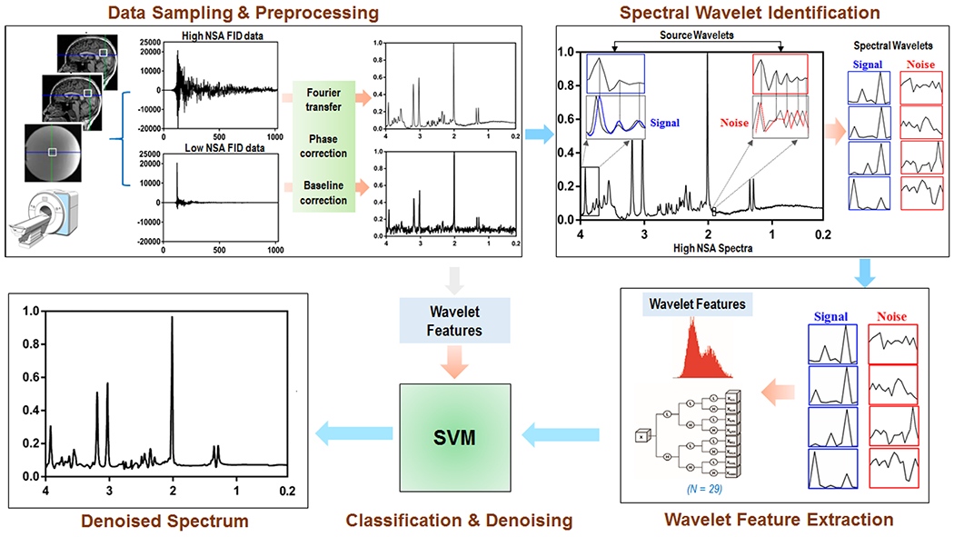
The flowchart illustrating the SWANCAD approach. Steps of the process include: pre-processing raw spectroscopy data, including Fourier transformation, phase and baseline correction; identifying the spectral wavelets from the input high NSA spectra based on source wavelets with specific waveforms or wavelets of spectral features representing noise and signal peaks for training the classification algorithm; extracting the spectral wavelets representing signals and noise from low NSA spectral data; using features of spectral wavelets of signals and noise and trained algorithm to classify the signal and noise peaks in the input low NSA spectral data; and removing noise while preserving the signal peaks when reconstructing the noise-removed spectrum.

Table 2.

Correlation coefficients of source wavelets and extracted spectral wavelets

Source Wavelets	Spectral Wavelet*	Correlation Coefficients R (p value)
		Phantom	Parietal Lobe	Temporal Lobe
Signal	1	0.94±0.01 (<0.01)	0.91±0.03 (<0.01)	0.89±0.05 (<0.01)
	2	0.96±0.02 (<0.01)	0.91±0.05 (<0.01)	0.90±0.06 (<0.01)
	3	0.95±0.01 (<0.01)	0.92±0.04 (<0.01)	0.88±0.07 (<0.01)
	4	0.96±0.01 (<0.01)	0.93±0.05 (<0.01)	0.87±0.06 (<0.01)
Noise	5	0.78±0.04 (<0.05)	0.68±0.06 (<0.05)	0.67±0.07 (<0.05)
	6	0.74±0.05 (<0.05)	0.66±0.07 (<0.05)	0.66±0.08 (<0.05)
	7	0.73±0.06 (<0.05)	0.67±0.06 (<0.05)	0.67±0.07 (<0.05)
	8	0.76±0.05 (<0.05)	0.65±0.05 (<0.05)	0.64±0.07 (<0.05)

^*The shape of each spectral wavelet presenting signals (blue, 1-4) and noise (red, 5-8) are presented in Figure 2.

Figure 3 shows the comparison of the contributions from 29 wavelet features of the spectral wavelets of the signals and noise. Among them, six were identified by SVM to have significant contributions to classification of signals and noise, including frequency or chemical shift, the integral of the signal peak, full width at half maximum (FWHM), signal amplitude, kurtosis, and range of frequency fluctuation. Statistically, they were shown to improve classification accuracy at 92.5, 90.8, 88.5, 87.3, 85.2, and 83.6 with statistically significant p-values at 0.001, 0.003, 0.006, 0.007, 0.01, and 0.03 for chemical shift, AUC, FWHM, amplitude, kurtosis, and range of frequency fluctuation, respectively. The combined effect of these six wavelet features in classification of signals and noise resulted in an overall accuracy of 95.7% as assessed by the SVM classifier with a combined polynomial kernel and RBF kernel function compared to accuracies achieved with each individual feature alone. The performances of the SVM classifiers with different kernels are summarized in Supplementary Table S1.

Figure 3.

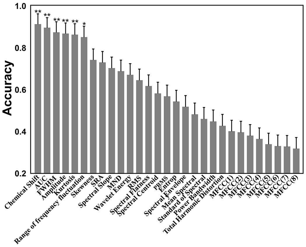
The accuracy of each wavelet feature in the spectral wavelets in contributing in the classification of signals and noises. *: p-value < 0.05, **: p< 0.01.

3.2. Denoising performance of the SWANCAD approach

Using the trained SWANCAD algorithm, low NSA spectra were processed to identify the signal and noise wavelets, which were then separated for subsequent denoising. As shown in the representative examples in Figure 4, the denoised spectra from temporal lobes of human brains exhibited improved spectral quality with clear enhancement in the conspicuity of the peaks from the metabolites of interest. These signal peaks match well with those of high NSA spectra collected in the same sampling volumes with same shimming and water suppression conditions but using much longer acquisition time.

Figure 4.

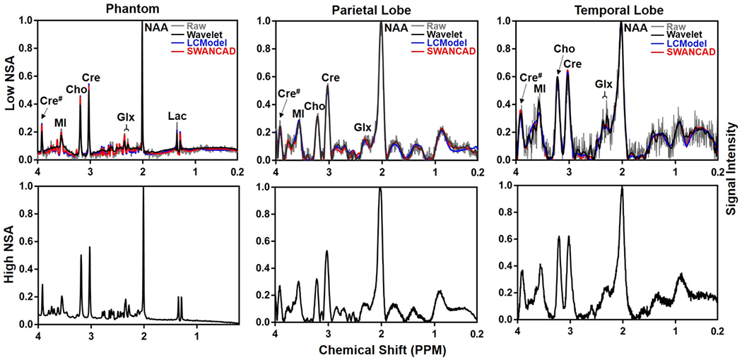
Comparisons of raw (grey) and denoised low NSA spectra (up row) with matching original high NSA spectra (low row) collected from the same sampling volumes of the phantom, parietal and temporal lobes of a healthy subject. Low NSA spectra were processed using LCModel (blue), SWANCAD (red), and wavelet threshold denoising (black) approaches, respectively

To quantitatively evaluate the denoising performance of the SWANCAD approach, SNRs were calculated for seven selected metabolite signals (i.e., NAA, Cre, Cho, MI, Lac and Glu+Gln or Glx) in all processed spectra. The plots in Figure 5 presents significant SNR improvements in low NSA spectra from both phantom and the parietal and temporal lobes of human brains before and after being denoised with the SWANCAD approach (p < 0.05). When comparing different denoising strategies using the same datasets, the SWANCAD approach exhibited slightly better performance than the LCModel, but a statistically significant improvement in SNR over that of the wavelet threshold method (Supplementary Table S2). In addition, the SWANCAD approach yielded better results than the wavelet threshold denoising algorithm in preserving the majority of prominent metabolites (i.e., NAA, Cre, Cho, Glx and MI) in the spectra of human parietal and temporal lobes.

Figure 5.

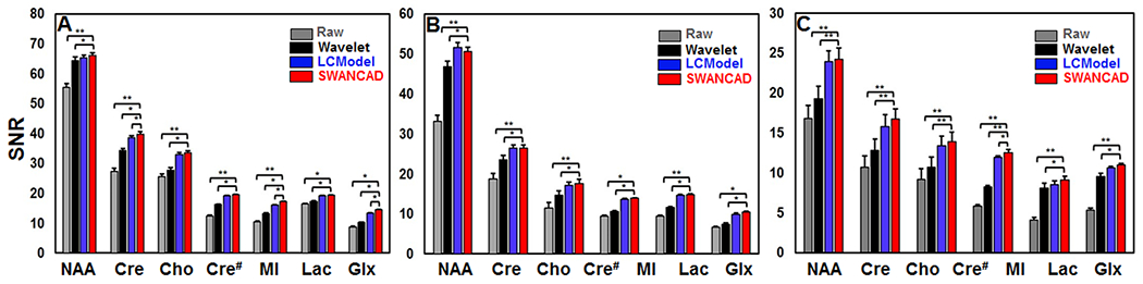
Comparison of SNRs of metabolites in spectra before and after being processed using LCModel, SWANCAD approach, and wavelet threshold denosing method. The spectra were recorded from phantom (A), parietal (B) and temporal (C) areas of human brains. *: p-value < 0.05, **: p-value < 0.01.

Importantly, when comparing the denoise performance of different denoising methods to the pure noise spectra, the SWANCAD approach was able to completely remove noise with an output baseline level of zero (Figure 6). As expected, the conventional wavelet threshold method only partially removed the noise. It is worth nothing that the “prior knowledge” based fitting process by LCModel effectively removed the noise in the areas where no metabolite peaks are expected. However, it also created unwanted “pseudo” metabolite peaks from the noise in the given chemical shifts where there may be anticipated common metabolites based on the prior knowledge. Adding the results from the denoise performance evaluation presented in Figure 5 and Table S2 together, the improved SNRs seen from applying the LCModel method may confound with artifacts from “undifferentiable” noise where the signals are expected from the prior knowledge.

Figure 6.

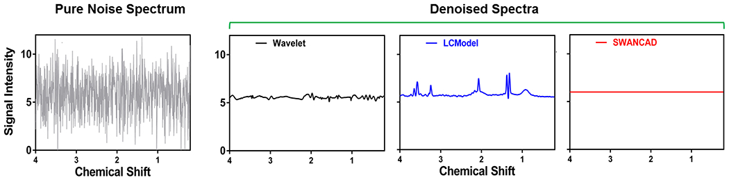
An example of a “noise-only” spectrum and the corresponding spectra fitted by LCModel and denoised by SWANCAD and wavelet threshold methods. The “noise-only” spectra were collected in a single voxel placed in the brain spectroscopy phantom. The “noise-only” spectra were recorded by turning off the RF power of the excitation pulse while other acquisition paramters and conditions remained the same during the run of the selected pulse sequence.

We then further tested whether denoising spectra affect the metabolite quantification based on the integrals of the methyl proton signal peak measured from seven selected metabolite signals (i.e., NAA, Cre, Cho, MI, Lac and the combined Glu and Gln or Glx) in all processed spectra and the metabolite concentration ratios calculated from the integral of methyl proton signal from a specific metabolite over that of Cre in the same spectra. Figure 7 summarizes the results from the measurement of integrals of methyl proton peaks of each selected metabolites in the high NSA spectra without applying any denoising process and low NSA spectra fitted or denoised by different methods. Specifically, in both data from the phantom (Figure 7A) and human parietal (Figure 7B) and temporal (Figure 7C) lobes, there was no statistically significant difference in measured metabolite levels between the non-denoised high NSA spectra and low NSA spectra denoised by the SWANCAD algorithm, indicating that the metabolite quantification was not compromised after low NSA spectra were denosing by SWANCAD. In comparison, the conventional wavelet threshold denoising method yielded significantly low levels of metabolites than those of non-denoised high NSA spectra and low NSA spectra denoised by SWANCAD (p < 0.05). The negative effect of denoising by the wavelet thereshold method on the metabolite quantification for NAA, Cho, Cre and Lac is even more pronounced in denoised spectra from the human parietal and temporal lobes, likely due to their lower SNR than those from the phantom. Worth noting, under the comparison analysis used in this study, the widely accepted LCModel method did not affect the metabolite quantification based on the statistical analysis of comparing the results obtained from high NSA spectra and LCModel processed low NSA spectra recorded in the same sampling voxels. Similar observations were obtained when using metabolite ratios based on the integrals of the methyl proton peaks of each metabolite against that of Cre (Figure S1).

Figure 7.

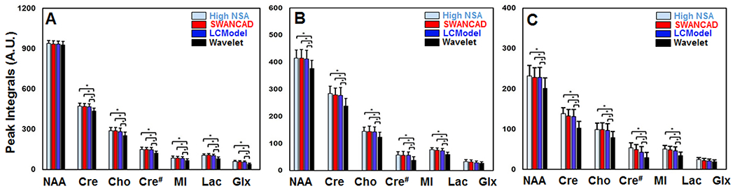
Comparisons of the results on the level of the selected metabolites measured by the integrals of selected –CH₃ methyl protons of each metabolite in different spectra obtained from the brain spectroscopy phantom (A), parietal lobe (B) and temporal lobe (C). Data from averaged high NSA spectra without denoising were used as the references. Low NSA spectra were processed and denoised using different methods as noted. No statistically significant difference between the non-denoised high NSA spectra and low NSA spectra denoised by the SWANCAD algorithm was found in measured metabolite levels. *: p-value < 0.05.

3.3. Application in Clinical Data

To demonstrate the potential benefit of the SWANCAD approach in the clinical applications of MRS, we tested its utility in denoising the single voxel spectra extracted from the individual voxels of CSI obtained from brain tumor patients. Because CSI exams were performed with NSA of 8 and FOV of 140 with the matrix of 16 x 16, the spectra extracted from a voxel of 8.8 x 8.8 x 20 mm³ from the CSI data is much smaller than the 20 x 20 x 20 mm³ voxel size used in the typical single voxel MRS exam. To evaluate the performance of denoising, we only selected the voxel well within the ROI of the CSI matrix of 16 x 16 as shown in Figure 8A. Given such small sampling volume and limited scan time, these spectra extracted from individual voxels in the CSI data usually have poor SNR. After applying the SWANCAD approach, the denoised spectra exhibited significantly improved SNRs (p < 0.01) in comparison with the original spectra (Figure 8B, C) when analyzing NAA, Cho and Cre, MI, and Lac, Glx signals. It is worth noting that after denoising, the noise-covered signal peaks in the region of 2.2-2.5 ppm, which are likely from Glx (i.e., overlapping glutamine and glutamate), become clearly distinguishable, further demonstrating the potential of the SWANCAD in recovering the signal peaks apparently overwhelmed by noise. In addition, SWANCAD significantly improve SNR (p < 0.05) in all selected metabolites when compared to that processed with LCModel and wavelet threshold denoising approach (Figure 8C). Although we observed the similar improvement in SNR after applying the SWANCAD and LCModel methods in processing low NSA spectra from the phantom and healthy brains using the same settings and processes as those used in analyzing data collected from the single voxels, SNR improvement by SWANCAD was significantly better (p < 0.05) than that by LCModel (p < 0.05) in processing metabolite peaks affected most by noise in the brain tumor patients.

Figure 8.

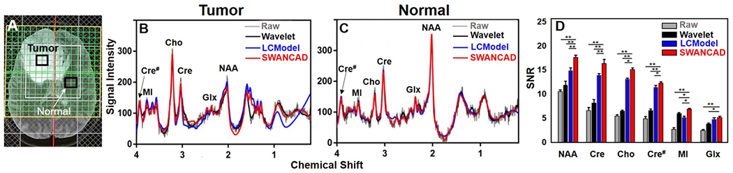
An example of applying SWANCAD to the individual spectra from the selected voxels of multi-voxel CSI data collected from a brain tumor patient. (A) ROI of the multi-voxel matrix overlapped on the axial T₂-wighted images showing a hyper-enhanced tumor in the left frontal area. Four individual spectra from the selected voxels (arrow pointed) in the tumor and four from the normal region were sel extracted for testing different denosing methods. Original and processed spectra from the tumor region (B) and from the normal region (C) after being spectral fitted by LCModel or denoised by SWANCAD or wavelet threshold denoising approaches, respectively. (D) Comparison of SNRs of metabolites in spectra before and after being processed using LCModel, SWANCAD and wavelet threshold approaches. Measurements were done and analyzed from a total of 16 spectra extracted from the tumor regions and 16 spectra from the normal regions of 4 patients. *: p-value < 0.05, **: p-value < 0.01.

4. Discussion

In this work, we presented the SWANCAD approach, a data-driven method employing a machine-learning classifier to distinguish the wavelet features of spectral wavelets representing noise and signal peaks in MR spectra. Using these wavelet features, the classification algorithm was able to effectively differentiate signal from noise, thereby enabling the removal of noise from the low NSA spectra to significantly improve SNR. Compared to traditional wavelet-based denoising methods⁴⁹, the reported SWANCAD approach uses much more parameters or features to evaluate and differentiate signal and noise, leading to improved denoising performance while retaining the metabolite peaks.

It was observed that the performance of denoising with SWANCAD generally dropped in going from the phantom data to those obtained from voxels in the parietal region and then the temporal region of human subjects. This is somewhat expected as the level of noise varies between the phantom and humans in which the tissue heterogeneity in the sampled volume and intrinsic physiological motions are inevitable^50,51. Despite this observation, the performance of the denoising approach was found to be consistent on data acquired from different subjects and voxel locations as indicated in Figure 5, which further validates the robustness of the SWANCAD when applied to the data collected in a variety of acquisition scenarios.

Compared to the conventional LCModel method widely used in MRS data analysis, the SWANCAD approach appears to have an advantage of differentiating and excluding noise, thus not “over estimating” metabolite signals, as LCModel, albeit a spectral fitting and not a denoising approach, may label and fit noise peaks at chemical shifts where metabolites are expected as “signals”. While this is not obvious in the denoised spectra containing brain metabolites, it is clearly demonstrated in processing pure noise spectra (Figure 6). Since the SWANCAD approach is data-driven rather than dependent on prior knowledges of metabolites, which is the basis of spectral fitting with the LCModel method, it provides more reliable information for metabolite quantification and detecting new metabolite signals that may not be included in the prior knowledge database. Importantly, our analysis on the effect of denosing on the metabolite quantification showed that the SWANCAD algorithm has the least effect on the results compared to other two denoising approaches, highlighting the advantage of the data-driven approach implemented in SWANCAD.

While MRS is an attractive non-invasive approach capable of providing molecular and metabolic information of the selected tissue volume without using exogeneous tracers or probes, its inherently limitted sensitivity has always been the major obstacle in its clinical applications, in which prolonging the scan time to gain higher SNR is not only intolerable to patients but also impractical for the clinical workflow. With continuous emphasis on precision and quantification in diagnosis and treatment monitoring, sampling small volume or increasing spatial resolution with spectroscopic imaging is highly desirable to analyze small abnormalities or heterogeneous lesions to avoid the partial volume effect. Advanced pulse sequences with novel data encoding schemes^{4, 5} and parallel receiver arrays are important approaches for shortening the acquisition time. The data-driven spectral denoising methods such as the reported SWANCAD should be complementary and can provide further enhancement in SNR without adding burdens in the patient tolerance and long scanner time. Such benefit of the SWANCAD denoising approach are best observed on the patient data (Figure 8), where the substantial noise levels in the original spectra limit the quantification of known metabolites, such as NAA, Cho and Cre, and detection of the low concentration or partially overlapped metabolites, such as Glx. However, denoised spectra provide sufficient spectral quality to mitigate both problems to reveal the diagnostic information otherwise buried in the noise.

Given the increasing interest and emerging methods in artificial intelligence-based approaches for improving image data processing and extracting quantitative information, the current study suggests several areas of improvement needed in the future investigations. A standardized validation including the high integrity signal data and noise data or “gold standards” would be needed. We only used the spectra with a high number of signal averages, i.e., high NSA, thus high SNR, as the reference standard. In addition, the SWANCAD was implemented and tested with two source wavelets selected visually based on their representativeness to the signal peaks and noise in the typical spectra. These wavelet sources may not be the optimal choices. A more quantitative means of identifying source wavelets based on large datasets to represent noise and signals in MRS data should result in even better performance in denoising and preserving peaks of low concentration metabolites. Finally, while the significant improvement in SNR was only observed in comparison between the low NSA and the denoised data, it is important to note that the SNR was only evaluated for the prominent signal peaks from the selected known metabolites. As discussed earlier, the application of the proper denoising methods based on the accurate classification of noise may also benefit the preservation of the signals from the low concentration metabolites or small signal peaks. Using an effective denoising approach to uncover or discover noise-contaminated signals can be important. The potential clinical significance of this will be further evaluated in a future study involving a larger cohort of patients with various data acquisition protocols.

5. Conclusion

The presented SWANCAD strategy offers an effective and efficient denoising method for gaining improved spectral quality with increased SNR from the noisy spectra acquired with low signal averaging and a short acquisition time to match the SNR of spectra obtained with high NSA and longer acquisition time. In addition, this denoising approach may allow for detecting and distinguishing the low intensity signals with substantial noise contamination. The excellent denoising performance without compromising the metabolite quantification by the SWANCAD method is achieved by identifying and extracting wavelet features using the machine-learning classification approach to differentiate the signals and noise of the original data. The SWANCAD approach therefore may assist MRS with the more accurate and more sensitive detection and quantification of metabolic abnormalities. The immediate impact of the SWANCAD in clinical applications is to enable underutilized MRS to overcome major limitations of low sensitivity and long acquisition time.

Abbreviations

AUC

Area under the curve

Cho

Choline

Cre

Creatine

CSI

Chemical shift imaging

CWT

Continuous wavelet transform

FID

Free induction decay

FLAIR

Fluid-attenuated inversion recovery

FWHM

Full width at half maximum

Glx

Glutamine+glutamate

Lac

Lactate

MPRAGE

Magnetization-prepared rapid acquisition gradient echo

MRI

Magnetic resonance imaging

MRS

Magnetic resonance spectroscopy

NAA

N-acetylaspartate

NSA

Number of signal averages

PCA

Principal component analysis

PRESS

Point resolved spectroscopy sequence

SNR

Signal to noise ratio

SWANCAD

Spectral Wavelet-feature Analysis and Classification Assisted Denoising

STEAM

Stimulated-echo acquisition mode

SVD

Singular value decomposition

SVM

Support vector machine

SVS

Single voxel spectroscopy

TE

Echo time

TR

Repetition time

TSE

Turbo spin echo

Data availability statement

The data from this study will be made available upon request.

REFERENCES

- 1.Dienel GA. Brain glucose metabolism: Integration of energetics with function. Physiol Rev. 2018; 99(1):949–1045. [DOI] [PubMed] [Google Scholar]
- 2.Shokrollahi P, Drake JM, Goldenberg AA. Signal-to-noise ratio evaluation of magnetic resonance images in the presence of an ultrasonic motor. Biomed Eng. 2017; 16(1):45. [DOI] [PMC free article] [PubMed] [Google Scholar]
- 3.Considine EC. The search for clinically useful biomarkers of complex disease: a data analysis perspective. Metabolites. 2019; 9:126–138. [DOI] [PMC free article] [PubMed] [Google Scholar]
- 4.Lam F, Li Y, Guo R, Clifford B, Liang ZP. Ultrafast magnetic resonance spectroscopic imaging using SPICE with learned subspaces. Magn Reson Med. 2020; 83(2):377–390. [DOI] [PMC free article] [PubMed] [Google Scholar]
- 5.Lam F, Ma C, Clifford B, Johnson CL, Liang ZP. High-resolution 1H-MRSI of the brain using SPICE: data acquisition and image reconstruction. Magn Reson Med. 2016; 76(4):1059–1070. [DOI] [PMC free article] [PubMed] [Google Scholar]
- 6.Baum KG. Signal filtering: noise reduction and detail enhancement. Handb Vis Disp Tech. 2012; 5:325–343. [Google Scholar]
- 7.Zhang Y, Zhou J, Bottomley PA. Minimizing lipid signal bleed in brain 1H chemical shift imaging by post-acquisition grid shifting. Magn Reson Med. 2015; 74(2):320–329. [DOI] [PMC free article] [PubMed] [Google Scholar]
- 8.Martin-Vaquero P, Da Costa RC, Echandi RL, Tosti CL, Knopp MV, Sammet S. Magnetic resonance imaging of the canine brain at 3 and 7T. Vet Radiol Ultrasound. 2011; 52:25–32. [PubMed] [Google Scholar]
- 9.Donoho DL, Johnstone JM. Ideal spatial adaptation by wavelet shrinkage. Biometrika. 1994; 81(3):425–455. [Google Scholar]
- 10.Wang CL, Zhang CL. Denoising algorithm based on wavelet adaptive threshold. Phys Procedia. 2012; 24:678–685. [Google Scholar]
- 11.Niu MS, Han PG, Song Lk, Hao DZ, Zhang JH, Ma L. Comparison and application of wavelet transform and Kalman filtering for denoising in δ13 CO2 measurement by tunable diode laser absorption spectroscopy at 2.008 µm. Optics express. 2017; 25:A896–A905. [DOI] [PubMed] [Google Scholar]
- 12.Kaur L, Gupta S, Chauhan R. Image denoising using wavelet thresholding. Conf Proc: Indian Conference on Computer Vision, Graphics and Image Processing (ICVGIP). 2002. [Google Scholar]
- 13.Zhang B, Sun L, Yu H, Xin Y, Cong Z. A method for improving wavelet threshold denoising in laser-induced breakdown spectroscopy. Spectrochimica Acta Part B. 2015; 107:32–44. [Google Scholar]
- 14.Cancino-De-Greiff HF, Ramos-Garcia R, Lorenzo-Ginori JV. Signal denoising in magnetic resonance spectroscopy using wavelet transforms. Concepts Magn Reson A. 2002; 14:388–401. [Google Scholar]
- 15.Ojanen J, Miettinen T, Heikkonen J, Rissanen J. Robust denoising of electrophoresis and mass spectrometry signals with minimum description length principle. Febs Lett. 2004; 570:107–113. [DOI] [PubMed] [Google Scholar]
- 16.Abdoli A, Stoyanova R, Maudsley AA. Denoising of MR spectroscopic imaging data using statistical selection of principal components. Magn Reson Mater Phy. 2016; 29:811–822. [DOI] [PMC free article] [PubMed] [Google Scholar]
- 17.Taswell C The what, how, and why of wavelet shrinkage denoising. Comput Sci Eng. 2000; 2(3):12–19. [Google Scholar]
- 18.Kasten J, Lazeyras F, Van De Ville D. Data-driven MRSI spectral localization via low-rank component analysis. IEEE Trans Med Imaging. 2013; 32:1853–1863. [DOI] [PubMed] [Google Scholar]
- 19.Komura D, Nakamura H, Tsutsumi S, Aburatani H, Ihara S. Multidimensional support vector machines for visualization of gene expression data. Bioinformatics. 2004; 21:439–444. [DOI] [PubMed] [Google Scholar]
- 20.Rivard B, Feng J, Gallie A, Sanchez-Azofeifa A. Continuous wavelets for the improved use of spectral libraries and hyperspectral data. Remote Sens Environ. 2008; 112:2850–2862. [Google Scholar]
- 21.Rafiee J, Tse P. Use of autocorrelation of wavelet coefficients for fault diagnosis. Mech Syst Signal PR. 2009; 23:1554–1572. [Google Scholar]
- 22.Silveira L Jr, Bodanese B, Zangaro RA, Pacheco MTT. Discrete wavelet transform for denoising Raman spectra of human skin tissues used in a discriminant diagnostic algorithm. Instrum Sci Technol. 2010; 38:268–282. [Google Scholar]
- 23.Du P, Kibbe WA, Lin SM. Improved peak detection in mass spectrum by incorporating continuous wavelet transform-based pattern matching. Bioinformatics. 2006; 22(17):2059–2065. [DOI] [PubMed] [Google Scholar]
- 24.Wee A, Grayden DB, Zhu Y, Petkovic Duran K, Smith D. A continuous wavelet transform algorithm for peak detection. Electrophoresis. 2008; 29(20):4215–4225. [DOI] [PubMed] [Google Scholar]
- 25.Qian F, Wu Y, Hao P. A fully automated algorithm of baseline correction based on wavelet feature points and segment interpolation. Opt Laser Technol. 2017; 96:202–207. [Google Scholar]
- 26.Rafiee J, Rafiee M, Prause N, Schoen M. Wavelet basis functions in biomedical signal processing. Exper Syst Appl. 2011; 38(5):6190–6201. [Google Scholar]
- 27.Tian D, Yang G. An automatic peak detection method for LIBS spectrum based on continuous wavelet transform. Spectrosc Spect Anal. 2014; 34(7):1969–1972. [PubMed] [Google Scholar]
- 28.Slavic J, Simonovski I, Boltezar M. Damping identification using a continuous wavelet transform: application to real data. J Sound Vib. 2003; 262:291–307. [Google Scholar]
- 29.Ogg RJ, Kingsley PB, Taylor JS. Wet, a T1- and B1-intensensitive water-suppression method for in vivo localized 1H NMR spectroscopy. J Magn Reson 1994; 104:1–10. [DOI] [PubMed] [Google Scholar]
- 30.Provencher SW. Estimation of metabolite concentrations from localized in vivo proton NMR spectra. Magn Reson Med. 1993; 30(6):672–679. [DOI] [PubMed] [Google Scholar]
- 31.Hu HB, Bai J, Xia G, Zhang W, Ma Y. Improved baseline correction method based on polynomial fitting for Raman spectroscopy. Photonic Sens. 2018; 8:332–340. [Google Scholar]
- 32.Sidhu KS, Khaira BS, Virk IS. Medical image denoising in the wavelet domain using Haar and DB3 filtering. Int J Eng Sci. 2012; 1:001–008. [Google Scholar]
- 33.Zhang X, Qi W, Cen Y, Lin H, Wang N. Denoising vegetation spectra by combining mathematical-morphology and wavelet-transform-based filters. J Appl Remote Sens. 2019; 13:016503. [Google Scholar]
- 34.Bayjja M, Boussouis M, Amar Touhami N. Studying the influence of the number vanishing moments of daubechies wavelets for the analysis of microstrip lines. Prog Electromagn Res. 2016; 62:57–64. [Google Scholar]
- 35.Caesarendra W, Tjahjowidodo T. A review of feature extraction methods in vibration-based condition monitoring and its application for degradation trend estimation of low-speed slew bearing. Machines. 2017; 5:21. [Google Scholar]
- 36.Muda L, Begam M, Elamvazuthi I. Voice recognition algorithms using mel frequency cepstral coefficient (MFCC) and dynamic time warping (DTW) techniques. ArXiv. 2010, 1003.4083. [Google Scholar]
- 37.Blagouchine IV, Moreau E. Analytic method for the computation of the total harmonic distortion by the Cauchy method of residues. IEEE T Commun. 2011; 59(9):2478–2491. [Google Scholar]
- 38.Chang CC, Lin CJ. LIBSVM: A library for support vector machines. ACM Trans Intell Syst Technol. 2011; 2:1–27. [Google Scholar]
- 39.Maldonado S, Weber R. A wrapper method for feature selection using support vector machines. Inf Sci. 2009; 179:2208–2217. [Google Scholar]
- 40.Sammut C, Webb GI. Leave-one-out cross-validation. Ency Mach Learn. 2010; 600–601. [Google Scholar]
- 41.Li S, Zhang Y, Xu J, et al. Noninvasive prostate cancer screening based on serum surface-enhanced Raman spectroscopy and support vector machine. Appl Phys Lett. 2014; 105(9):091104. [Google Scholar]
- 42.Xie T, Yao J, Zhou Z. DA-based parameter optimization of combined kernel support vector machine for cancer diagnosis. Processes. 2019; 7(5):263. [Google Scholar]
- 43.Fleischer CC, Zhong XD, Mao H. Effects of proximity and noise level of phased array coil elements on overall signal-to-noise in parallel MR spectroscopy. Magn Reson Imaging. 2018; 47:125–130. [DOI] [PMC free article] [PubMed] [Google Scholar]
- 44.Deelchand DK, Kantarci K, Öz G. Improved localization, spectral quality, and repeatability with advanced MRS methodology in the clinical setting. Magn Reson Med. 2018; 79:1241–1250. [DOI] [PMC free article] [PubMed] [Google Scholar]
- 45.Lu JY, Lin H, Dong Y, Zhang YS. A new wavelet threshold function and denoising application. Math Probl Eng. 2016; 2016:1–8. [Google Scholar]
- 46.Basu S, DasGupta A. The mean, median, and mode of unimodal distributions: a characterization. Theor Probab Appl. 1997; 41(2):210–223. [Google Scholar]
- 47.Dodge Y The concise encyclopedia of statistics. Springer Sci & Bus Media; 2008. [Google Scholar]
- 48.Kobus T, Wright AJ, Weiland E, Heerschap A, Scheenen TW. Metabolite ratios in 1H MR spectroscopic imaging of the prostate. Magn Reson Med. 2015; 73(1):1–12. [DOI] [PubMed] [Google Scholar]
- 49.Zhang L, Bao P, Pan Q. Threshold analysis in wavelet-based denoising. Electron Lett. 2001; 37(24):1485–1486. [Google Scholar]
- 50.Wang Y, Day SM. Seismic source spectral properties of crack-like and pulse-like modes of dynamic rupture. J Geophys Res. 2017; 122(8):6657–6684. [Google Scholar]
- 51.Dienel GA. Brain glucose metabolism: integration of energetics with function. Physiol Rev. 2019; 99(1):949–1045. [DOI] [PubMed] [Google Scholar]
Associated Data
This section collects any data citations, data availability statements, or supplementary materials included in this article.
Supplementary Materials