Length-biased semi-competing risks models for cross-sectional data: an application to current duration of pregnancy attempt data

Abstract

Cross-sectional length-biased data arise from questions on the at-risk time for an event of interest from those who are at-risk but have yet to experience the event. For example, in the National Survey on Family Growth (NSFG), women who were currently attempting to become pregnant were asked how long they had been attempting pregnancy. Cross-sectional survival analysis methods use the observed at-risk times to make inference on the distribution of the unobserved time-to-failure. However, methodological gaps in these methods remain such as how to handle semi-competing risks. For example, if the women attempting pregnancy had undergone fertility treatment during their current pregnancy attempt. In this paper, we develop statistical methods that extend cross-sectional survival analysis methods to incorporate semi-competing risks. They can be used to estimate the distribution of the length of natural pregnancy attempts (i.e., without fertility treatment) while correctly accounting for women that sought fertility treatment prior to being sampled using cross-sectional data. We demonstrate our approach based on simulated data and an analysis of data from the NSFG. The proposed method results in separate survival curves for: time-to-natural-pregnancy, time-to-fertility treatment, and time-to-pregnancy after fertility treatment.

1. Introduction

Cross-sectional studies of time-to-event outcomes occur when data are observed on the right-censored time for an event of interest, from those currently at-risk. Such length-biased cross-sectional survival data are seen in studies of time-to-pregnancy (TTP) (Weinberg and Gladen, 1986; Keiding et al., 2002; McLain et al., 2014), residential migration (Allison, 1985; Yamaguchi, 2003), length of hospitalization time after surgery (Mandel and Rinott, 2014; Mandel, 2015) and survival of dementia patients (Bergeron et al., 2008; Carone et al., 2014). The benefits of cross-sectional time-to-event designs include that it may be easier to sample people while they are currently at-risk (e.g., with hospitalization patients), are more cost and time effective then prospective studies and they will include subjects that never experienced the event (missing from some retrospective TTP studies, Scheike and Keiding, 2006). A difficulty with data arising from such studies is that the responses are length biased (subjects with longer event times are more likely to be at-risk) and entirely right censored since all subjects have not experienced the event of interest.

Cox (1969) originally developed the survival analysis theory for how to provide inference on the unobserved event of interest (see van Es et al., 2000, for a formal derivation). Parametric survival models have been considered by Allison (1985), Weinberg and Gladen (1986), Keiding et al. (2002) and Keiding et al. (2012), among others. It is possible that a time-dependent intermittent event occurs during some subjects’ at-risk periods. That is, between the start of the at-risk period and the sampling time the subject experienced an intermittent event that changed the failure rate. The semi-competing risks framework (also referred to as the illness-death model) can handle this type of data. Mandel and Fluss (2009) and Mandel (2010) considered a competing risks illness–death model under cross-sectional sampling to estimate the probability of illness and the rates of illness and death among hospitalized patients. Their methods, however, required follow-up on the total event time which will not be available in some cross-sectional studies. Keiding (1991) considered a situation very similar to that given here (see Section 6 therein) though he does not give a full treatment of the problem.

In this paper, we develop statistical methods that can be used to analyze cross-sectional length-biased survival data that are subjected to semi-competing risks. Our methods only require data available at the cross-sectional sampling time. We use a piecewise constant hazard model to estimate the underlying distribution of the event of interest and the semi-competing risk. We use a latent variable treatment of the semi-competing risks where the inference is based on the latent outcomes, which some have critiqued as lacking real world interpretability (Andersen and Keiding, 2012). An alternative approach is to model the cumulative incidence function or subdistribution, based on the joint probability of the outcome and event type (Fine and Gray, 1999; Fine et al., 2001). The motivation for using the latent variable framework is that the theoretical outcome of interest from this model coincides with TTP if fertility treatment were not an option. This outcome is representative of fecundity, the biologic ability to achieve pregnancy. Alternatively, the subdistribution of TTP and not entering fertility treatment has less biologic relevance. We do note that modeling the cumulative incidence function is more preferable for the other outcomes. For example, Duron et al. (2013) estimate the cumulative incidence function medical consultation for fecundity problems. TTP if fertility treatment were not an option is a counterfactual outcome, which calls for causal inference survival analysis methods. These methods have strong assumptions that may be hard to justify with the available data (discussed more in Section 7). As a result, in this paper we focus on estimating the distribution of TTP while correcting for the informative censoring caused by infertility treatment through a semi-competing risks model.

The outline of the paper is as follows. In Section 2, we introduce the motivating data set and the application of interest. In Section 3, we discuss the standard theory for cross-sectional length biased data, give the assumptions of the procedure, and derive the densities and likelihood when semi-competing risks are present. In Section 4, we present an approach to incorporate dependence between the latent variables. In Section 5, we present results from simulation studies. In Section 6, we apply our methods to data from the National Survey on Family Growth (NSFG) to estimate the distribution of TTP while correctly accounting for women that have undergone fertility treatment (the semi-competing risk) and compare our results to competing methods. We conclude with some discussion.

2. Motivating Data

Cross-sectional data on the length of pregnancy attempt are used in reproductive epidemiology to estimate the survival curve of TTP, a technique that has been referred to as the current duration approach (Keiding et al., 2002). The data arise when women are asked, “Are you currently trying to get pregnant” and if the woman said ‘yes,’ “How long have you been currently attempting pregnancy?” The responses to the latter question are referred to as the woman’s current duration of pregnancy attempt. In the NSFG, women are also asked to list the dates and types of fertility treatment, which complicates the analysis if fertility treatment occurred during the current attempt. That is, the moment a woman began fertility treatment, her ‘natural’ pregnancy attempt stopped and her pregnancy attempt on fertility treatment began.

The conceptual data model for a successful pregnancy attempt is presented in Figure 1 where T represents the time-to-natural-pregnancy, which we refer to TTNP, Y is the time-to-fertility treatment (TTFT) and Z the time-to-pregnancy after fertility treatment (TTPFT) where Z = 0 if T < Y. This is viewed as a semi-competing risks problem or through the illness-death model, since fertility treatment always occurs before pregnancy, but does not always occur. Here, TTP is used to denote time-to-pregnancy which could be aided by fertility treatments. We note that pregnancy attempts can be ‘unsuccessful’ and end for other reasons (e.g., giving up). That is, either a natural pregnancy attempt or a pregnancy attempt after fertility treatment can end without the women getting pregnant. The current duration approach provides inference on the end of attempts and cannot differentiate between ‘successful’ and ‘unsuccessful’ pregnancy attempts (Keiding et al., 2002, 2012).

Figure 1:

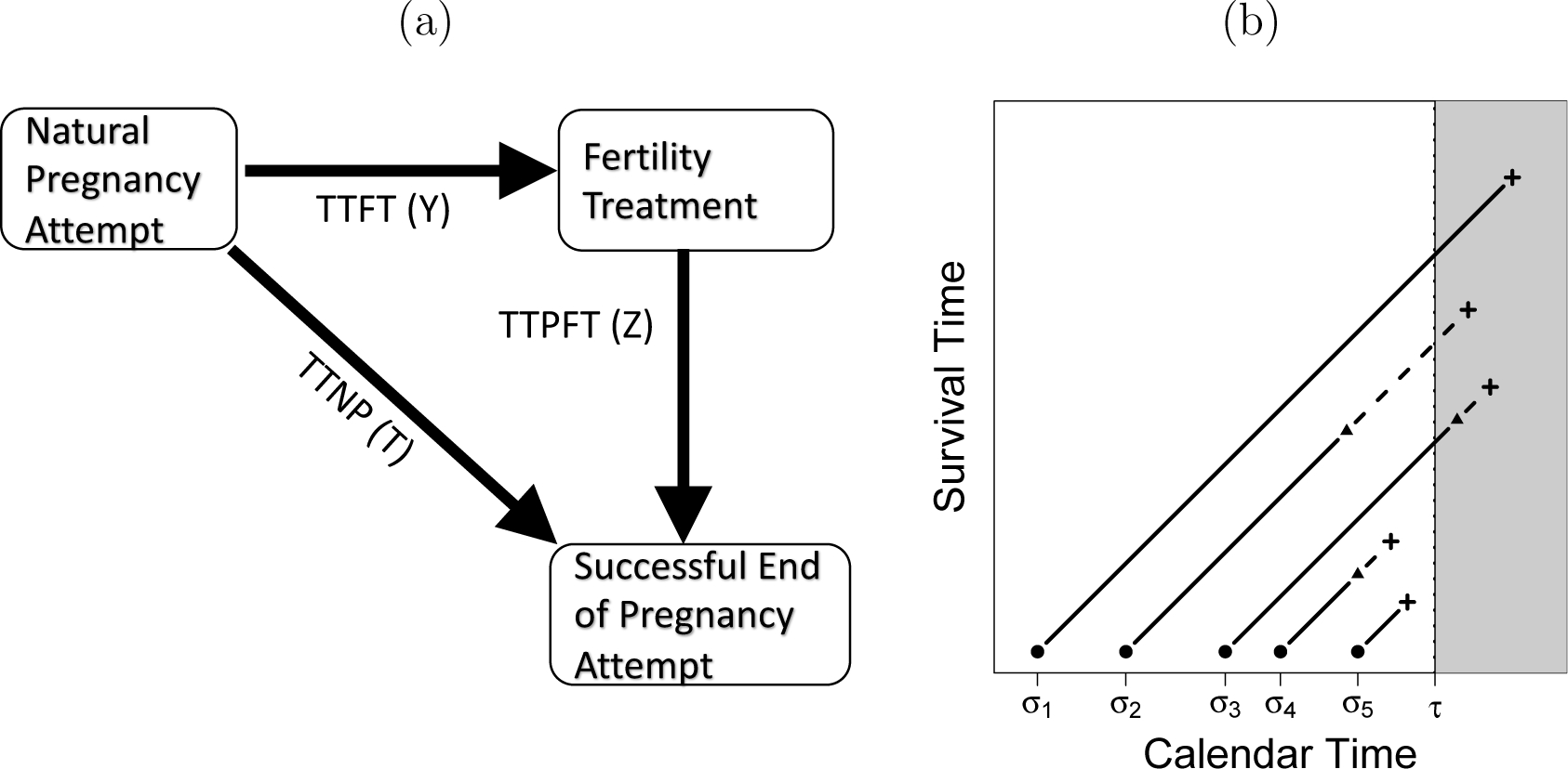
(a) Graphical representation of the illness-death model of a successful pregnancy attempt with time-to-natural-pregnancy (TTNP), time-to-fertility treatment (TTFT) and time-to-pregnancy on fertility treatment (TTPFT). (b) Lexis diagram for five subjects with their start of their at-risk period • (σ_i), time of their intermittent event ▲, time of the event of interest +, and the time of cross-sectional sampling τ. Events in the gray area of the figure are not observed.

As opposed to the standard semi-competing risks scenario, in a cross-sectional sample we observe the current at-risk period and the time (if any) that the intermittent event occurred. For example, let σ denote the time the woman’s pregnancy attempt begins and τ the sampling time. Without loss of generality, we assume that τ is equal across subjects. In cross-sectional data, we only observe what occurred before τ for subjects at risk at τ.

The observed data are displayed in Figure 1 for five hypothetical women as a Lexis diagram. Events that occur in the gray area of the figure are unobserved with cross-sectional data. For example, with women 1 and 3 we observed the current length of their natural pregnancy attempts. For woman 2, we observe the TTFT (Y) and the current duration of their fertility treatment. At τ it is not known that woman 1 will get pregnant naturally and woman 3 will enter fertility treatment. No data from women 4 or 5 are observed since they are not at-risk for pregnancy when surveyed. This is a unique feature that sets it apart from standard length-biased survival data where subjects are followed from τ to the event of interest or censoring.

3. Methods

This section begins with the data notation and an overview of the derivation of the likelihood function for a general dependence structure (full details are given in Section B of the Supplemental Materials). We then give simplifications of the likelihood under various dependence scenarios.

3.1. Notation, assumptions and likelihood

The observed data consist of independent realizations of ${\mathcal{D}}_i=\left\{X_i,Z_i^{*},{\delta }_i\right\}$ for i = 1, 2, … , n, where X_i is the observed time at risk (i.e., τ_i − σ_i in Figure 1), $Z_i^{*}$ is the time since the intermittent event where $Z_i^{*}=0$ if the intermittent event has not occurred, and $I(Z_i^{*}>0)$ for subject i. For ease of notation, let Y denote the time to the intermittent event. Note that Z^∗ is the observed time since the intermittent event (i.e., the at-risk time since the intermittent event), while Z is the (unobserved) full time from the intermittent event until failure. If δ_i = 0, then X_i represents the current duration of T_i ∧ Y_i where T ∧ Y = min(T, Y). If δ_i = 1, we observe Y_i and $Z_i^{*}$. We use f, F, $\overline{F}$ to denote a generic probability measure, distribution function and survival function, respectively, and subscript the appropriate random variable. Our derivation of the observed data likelihood extends results given by Dauxois et al. (2014) on length-biased competing risks data and arguments given by Vardi (1989). Most of the technical details of the derivation are given in the Supplemental Materials, here we outline the main concepts.

Our formation of the likelihood uses some important regularity conditions. Throughout we assume that (a) the beginning of the at-risk periods (σ_i) are governed by a homogeneous Poisson process with rate ψ, and (b) conditional on σ_i the distributions of T, Y and Z are independent of calendar time (we discuss these assumptions further in Section 6 and Section A of the Supplemental Materials).

For δ = 0 the derivation of the likelihood follows standard current duration results. Given δ = 0, the results of Cox (1969) can be used to derive the form of the distribution of X|δ = 0. Further, in the appendix we derive Pr(δ = 0). In total, for those with δ = 0 the likelihood contribution is

$$f_{X,\delta }(x,0)=\frac{{\overline{F}}_{T\wedge Y}(x)}{E(T\wedge Y+Z)}.$$ (1)

The forms for ${\overline{F}}_{T\wedge Y}$ and E(T ∧ Y + Z) are discussed below.

To derive the likelihood contribution for δ = 1, it is useful to first consider the case where Z is fully observed (i.e., if followup past τ were available) then use results on multiplicative censoring (Vardi, 1989) to obtain the density for the observed cross-sectional data at τ. In the Supplemental Material, we show that the likelihood of (Y, Z, δ = 1) is

$$f_{Y,Z,\delta }(y,z,1)=\frac{{\int }_y^{\infty }z{f}_{T,Y,Z}(u,y,z)du}{E(T\wedge Y+Z)}.$$ (2)

Since Z occurs last in the temporal ordering of the variables it is most natural to consider the distribution of Z|X, Y, and represent the integrand in (2) as zf_T,Y,Z(t, y, z) = zf_Z|T,Y (z)f_T,Y (t, y) where, for brevity, we use f_Z|T,Y(z) = f_Z|T=t,Y=y(z) throughout. Given the steady state assumptions, δ = 1 and Y, we were equally likely to observe the current duration of Z at any time point (van Es et al., 2000). As a result, the observed cross-sectional variable $Z^{*}\stackrel{d}{=}U\tilde{Z}$ where U ∼Uniform(0, 1), $\tilde{Z}\stackrel{d}{=}Z\mid (Y,\delta =1)$ and $\stackrel{d}{=}$ denotes equal in distribution. Following these results we obtain the likelihood contribution of (Y, Z^∗, δ = 1) as

$$f_{Y,Z*}{}_{,\delta (y,z,1)}=\frac{{\int }_y^{\infty }{\overline{F}}_{Z\mid T,Y}(z)f_{T,Y}(u,y)du}{E(T\wedge Y+Z)}$$ (3)

(see the Supplemental Materials for a formal derivation).

Combining the above results, and using the form for E(T∧Y+Z) given in the appendix, the full likelihood is given by

$$L\left({\mathcal{D}}_i\mid \theta \right)\propto \frac{{\overline{F}}_{T\wedge Y}{\left(X_i\right)}^{\left(1-{\delta }_i\right)}{\left\{{\int }_{Y_i}^{\infty }{\overline{F}}_{Z\mid T,Y}\left(Z_i^{*}\right)f_{T,Y}\left(u,Y_i\right)du\right\}}^{{\delta }_i}}{\int {\overline{F}}_{T\wedge Y}(u)du+{\iint }_u^{\infty }E(Z\mid T,Y)f_{TY}(v,u)dvdu},$$ (4)

with θ = {F_T, F_Y, F_Z, R} ⊂ Θ denoting the parameters where R denotes the dependence parameters (discussed further in Section 4). Performing maximum likelihood analysis of the complete data $\mathcal{D}=\left\{{\mathcal{D}}_1,{\mathcal{D}}_2,\dots ,{\mathcal{D}}_n\right\}$ amounts to maximizing $l(\theta \mid \mathcal{D})={\sum }_{i=1}^n\log \left\{L\left({\mathcal{D}}_i\mid \theta \right)\right\}$ with respect to θ such that θ ⊂ Θ.

3.2. Likelihood under various dependence assumptions

It is common that semi-competing risks will have dependence through direct relationships or unobserved covariates. Below we discuss how the form of the likelihood in (4) can be simplified under some independence assumptions. Under complete independence, i.e., T ⊥ Y, T ⊥ Z and Y ⊥ Z where ⊥ denotes independence, we have

$$L_C\left({\mathcal{D}}_i\mid \theta \right)\propto \frac{{\left\{{\overline{F}}_T\left(X_i\right){\overline{F}}_Y\left(X_i\right)\right\}}^{\left(1-{\delta }_i\right)}{\left\{{\overline{F}}_T\left(Y_i\right)f_Y\left(Y_i\right){\overline{F}}_Z\left(Z_i^{*}\right)\right\}}^{{\delta }_i}}{\int {\overline{F}}_T(u){\overline{F}}_Y(u)du+E(Z)\int {\overline{F}}_T(u)f_Y(u)du}.$$

A more realistic assumption is to assume that Z ⊥ (T, Y), but still model the dependence between T and Y. In this case, the likelihood is

$$L_Z\left({\mathcal{D}}_i\mid \theta \right)\propto \frac{{\overline{F}}_{T\wedge Y}{\left(X_i\right)}^{\left(1-{\delta }_i\right)}{\left\{{\overline{F}}_{T\mid Y}\left(Y_i\right)f_Y\left(Y_i\right){\overline{F}}_Z\left(Z_i^{*}\right)\right\}}^{{\delta }_i}}{\int {\overline{F}}_{T\wedge Y}(u)du+E(Z)\int {\overline{F}}_{T\mid Y}(u)f_Y(u)du}.$$ (5)

This assumption leads to a relatively computationally friendly likelihood (similar to complete independence), but Z ⊥ (T, Y) could be a strong assumption in practice.

Lastly, we considered two conditional independence assumptions. First, suppose T ⊥ Z|Y, that is T and Z are conditionally independent given Y. In this case, the likelihood is

$$L_{TZ\mid Y}\left({\mathcal{D}}_i\mid \theta \right)\propto \frac{{\overline{F}}_{T\wedge Y}{\left(X_i\right)}^{\left(1-{\delta }_i\right)}{\left\{{\overline{F}}_{T\mid Y}\left(Y_i\right)f_Y\left(Y_i\right){\overline{F}}_{Z\mid Y}\left(Z_i^{*}\right)\right\}}^{{\delta }_i}}{\int {\overline{F}}_{T\wedge Y}(u)du+\int E(Z\mid Y){\overline{F}}_{T\mid Y}(u)f_Y(u)du}.$$ (6)

Second, consider Y ⊥ Z|T, which results in

$$L_{YZ\mid T}\left({\mathcal{D}}_i\mid \theta \right)\propto \frac{{\overline{F}}_{T\wedge Y}{\left(X_i\right)}^{\left(1-{\delta }_i\right)}{\left\{{\int }_{Y_i}^{\infty }{\overline{F}}_{Z\mid T}\left(Z_i^{*}\right)f_{T,Y}\left(u,Y_i\right)du\right\}}^{{\delta }_i}}{\int {\overline{F}}_{T\wedge Y}(u)du+\int E(Z\mid T)F_{Y\mid T}(v)f_T(v)dv}.$$ (7)

Assuming forms for all conditional distributions and expectations are available, it is evident that assuming T ⊥ Z|Y adds a relatively small amount of computational intensity over the Z ⊥ (T, Y) or complete independence assumptions and has a more flexible dependence structure. The Y ⊥ Z|T assumption adds computational complexity due to the additional integral in the numerator. Both conditional independence assumptions have considerable computational advantage over the general dependence structure. Particularly, the denominator of (4) is computationally demanding due to the double integral of E(Z|T, Y) (which must be evaluated numerically). As a result, we focus on the Y ⊥ Z|T assumption which (as discussed in Section 6) is well-motivated by our motivating example.

4. Dependence and Distributional Specifications

Building on the results from the previous section, we wish to model the dependence of (T, Y, Z) such that forms for conditional distributions are available and flexible to various dependence assumptions. Further, in our motivating example, the hypothesized direction of the dependence between T and Y is negative, in that those with longer TTNP would have shorter TTFT. As a result, we consider a dependence structure that is amenable to positive or negative dependence. The Gaussian copula is particularly appealing since it incorporates negative dependence, has straightforward representations of conditional distributions and can incorporate conditional independence. The three-dimensional Gaussian copula is stated as

$$C_R\left(u_1,u_2,u_3\right)={\mathrm{\Phi }}_R\left\{{\mathrm{\Phi }}^{-1}\left(u_1\right),{\mathrm{\Phi }}^{-1}\left(u_2\right),{\mathrm{\Phi }}^{-1}\left(u_3\right)\right\},$$

where Φ⁻¹ is the inverse distribution function of a standard normal and Φ_R represents the distribution function of a multivariate Gaussian distribution with mean 0 and correlation matrix R with elements r_ij. The joint distribution function is given by Pr(T ≤ t, Y ≤ y, Z ≤ z) = C_R{F_T(t), F_Y(y), F_Z(z)}.

The conditional independence assumptions discussed in Section 3.2 can be made by setting specific portions of R⁻¹ to zero. To form the conditional distributions let W_T = Φ⁻¹{(F_T(T)}, similarly for W_Y and W_Z. The distribution function of W_Z|(W_T,W_Y) is given by

$$\mathrm{Pr}\left(W_Z\le w_z\mid {\mathit{W}}_{TY}={\mathbf{w}}_{TY}\right)=\mathrm{\Phi }\left(\frac{w_{j+1}-{\mathit{r}}_Z^{\prime }{\mathit{R}}_{TY}^{-1}{\mathit{w}}_{TY}}{{\sigma }_{Z\mid TY}}\right)$$ (8)

where W_TY = (W_T, W_Y), ${\mathit{R}}_{TY}^{-1}$ is the inverse correlation matrix of W_TY, r_Z = (r_TZ, r_YZ) are the correlations between (W_T, W_Y) and W_Z, and ${\sigma }_{Z\mid TY}^2=1-{\mathit{r}}_Z^{\prime }{\mathit{R}}_{TY}^{-1}{\mathit{r}}_Z$. The density and distribution functions of all the required conditional distributions can be formed following (8). For both simulations and real data analysis we assumed the direction of the dependence was known and appropriately modified the parameter space of the correlation parameters.

To model the marginal distributions of T, Y, and Z we seek a form that is flexible and amendable to the properties of the data in our motivating example. McLain et al. (2014) noted that data from the NSFG is subject to digit preference at 6, 12, 18, etc., months. They proposed a piecewise constant hazard model with knot selection designed to minimize the effect of digit preference. The cumulative hazard function for the piecewise constant hazard model states that $H(t\mid \mathbf{\alpha },\mathbf{t})={\sum }_{\left\{j:t_{j-1}<t\right\}}{\alpha }_j\left\{\left(t\wedge t_j\right)-t_{j-i}\right\}$, where t = (t₀, t₁, t₂, … , t_L) denote the knot locations with 0 ≡ t₀ < t₁ < … < t_L ≡ ∞, α = (α₁, … , α_L) and α_j is the hazard rate over [t_j−1, t_j). The survival functions for T, Y, and Z are given by $\overline{F}\left(\cdot \mid {\mathbf{\alpha }}_T,{\mathbf{t}}_T\right)$, $\overline{F}\left(\cdot \mid {\alpha }_Y,t_Y\right)$, and $\overline{F}\left(\cdot \mid {\mathbf{\alpha }}_Z,{\mathbf{t}}_Z\right)$ where $\overline{F}(t\mid \mathbf{\alpha },t)=\exp \{-H(t\mid \mathbf{\alpha },t)\}$.

The main computational challenges of the likelihood in (7) (which we mainly focus on) is computing the integrals in the numerator and in the later part of the denominator. Neither can be simplified outside of a full Gaussian assumption. A Taylor series approximation (up to fourth order) was attempted to simplify the E(Z|T) expectation but was found to be unsatisfactory. As a result, we considered two estimation strategies: i) a mixed quadrature approach with Legendre quadrature for the integral in the numerator and a mix of Legendre quadrature and adaptive quadrature in the denominator, and ii) full adaptive quadrature, which is much more computationally demanding. The accuracy of the likelihood approximation methods was compared to the Z ⊥ (T, Y) likelihood in (5) (where calculations are straightforward) for a variety of situations under the Z ⊥ (T, Y) assumption. This comparison showed that full adaptive quadrature was more accurate than mixed, particularly with skewed distributions. In our simulations, we use the mixed quadrature approach since it had satisfactory results and markedly shorter computation time. In the data analysis, we calculated the likelihood using the slower, more accurate full adaptive quadrature. All code was written in the R environment (R Core Team, 2020) and is available in the Supplemental Material and online at https://github.com/alexmclain/CDSCR.

Identifiability is an important issue in competing risk models. There is a well-known identifiability issue with dependent competing risks (Tsiatis, 1975), where multiple marginal distributions and dependence specifications can result in equivalent models. As a result, the estimated marginal distributions are reliant on a correct specification of the dependence structure. As discussed in Section A of the Supplementary Materials, the two main assumptions discussed in the beginning of Section 3.1 are needed to identify the parameters. Briefly, assumption (a) implies that the probability a subject was included in the sample is proportional to their total survival time, which relates the desired variable T to a length biased version of T (this assumption can be relaxed if data on the start of events are available). Further, assumption (b) is used to control for the censoring and implies multiplicative censoring by a uniform random variable. These assumptions are vital to relating the observed data to the random variables of interest.

5. Simulation Studies

To test the properties of the proposed method, numerous simulation studies were run. The simulation studies were run by simulating data for T, Y and Z using distributions designed to closely resemble their underlying biological processes in the motivating example. The current duration data were generated using methods described in McLain et al. (2014). The data were simulated using via two distributional assumptions. The first used the assumed piecewise constant hazard model discussed in Section 4, where t_T = {2, 5, 9, 14}, t_Y = {6, 9, 12}, and t_Z = {2, 10} with the following rates log(α_T) = (−2.5, −2.375, −2.25, −2.125, −2), log(α_Y) = (−3.5, −3.0, −2.0, −1.5) and log(α_Z) = (−1, −2, −3). The second setting used a Weibull(k, λ) distribution with mean λΓ(1 + 1/k) where (k, λ) were set to (3/4, 6), (4, 10) and (3/4, 2) for T, Y and Z, respectively. The data were generated using a Gaussian Copula with the following pairs of (ρ_TY, ρ_TZ): (−0.2, 0.2), (−0.4, 0.4), (−0.6, 0.6), (−0.2, 0.6), (−0.2, 0.4) and (−0.4, 0.6). Here, ρ_YZ = ρ_TY ρ_TZ under the Y ⊥ Z|T assumption. Additional simulations which considered a t Copula and other dependence scenarios are presented in the Section C of the Supplementary Material (conclusions were similar to below). All simulations used n = 1, 000 for 500 iterations.

The knot locations were set to the percentiles of the observed X_i, Y_i and $Z_i^{*}$ data. For the piecewise constant model the number of knots was equal to the true number of knots, while for the Weibull setting each distribution used 8 knots. Starting values of the parameters were obtained using a standard current duration approach applied to the X_i and Z_i data for α_T and α_Z, respectively, while α_Y was set such that it resulted in the percentiles observed from Y_i.

We compare our model a ‘standard’ piecewise constant current duration model which analyzes the data without correction (knots and starting values chosen the same way). That is, the observed X data are analyzed using McLain et al. (2014) ignoring the Z information. We also tested other approaches where subjects that experience the intermediate event were adjusted using a covariate or dropped. For the data simulated here, these resulted in estimates with markedly worse properties. We discuss these standard approaches more thoroughly in Section A of the Supplemental Material.

In Tables 1 and 2, we present the bias of the average estimated survival function along with Monte Carlo standard error (SE) for select values of t. For the piecewise constant data, the proposed method has relatively small bias when estimating the survival function of T, the main parameter of interest, regardless of the dependence parameters. This suggests that the proposed method can estimate the distribution of T with low bias and is robust to misspecification in the knot locations. The standard approach resulted in uniformly more bias than the proposed model. The bias for the standard approach at t = 12 (a point of interest in our application) ranged from −0.059 to −0.102. For the proposed model estimates of the distribution for Y and Z performed well overall, but there does appear to be some bias in the at t = 24 for Y and t = 3 for Z (see Section C of the Supplementary Materials for figures of the estimated and true survival curves). The results suggest the method has some difficulty estimating the correlation parameters, though all had bias less than SE/2.

Table 1:

Simulation results of the proposed procedure along with a standard approach for data simulated with a piecewise constant hazard and n = 1, 000. Displayed is the average bias (BIAS) and Monte Carlo standard error (SE) of ${\overline{F}}_T(t)$ (estimated for both approaches), along with ${\overline{F}}_Y(t)$, ${\overline{F}}_Z(t)$ and ρ_xy, ρ_xz (estimated with the proposed method only).

		ρTY = −0.2	ρTY = −0.4	ρTY = −0.6	ρTY = −0.2
		ρTZ = 0.2	ρTZ = 0.4	ρTZ = 0.6	ρTZ = 0.6
t	True	bias(se)	bias(se)	bias(se)	bias(se)
		Standard Method
		${\overline{F}}_T(t)$
3	0.773	−0.036 (0.081)	−0.028 (0.084)	−0.039 (0.079)	−0.025 (0.082)
6	0.578	−0.053 (0.059)	−0.054 (0.065)	−0.054 (0.058)	−0.042 (0.061)
12	0.294	−0.102 (0.021)	−0.076 (0.025)	−0.083 (0.022)	−0.059 (0.027)
24	0.060	0.013 (0.008)	0.037 (0.011)	0.028 (0.009)	0.045 (0.012)
		Proposed Method
		${\overline{F}}_T(t)$
3	0.773	−0.007 (0.097)	0.002 (0.098)	−0.003 (0.100)	0.010 (0.104)
6	0.578	−0.011 (0.074)	0.001 (0.076)	−0.006 (0.079)	0.003 (0.084)
12	0.294	−0.016 (0.063)	−0.013 (0.068)	−0.014 (0.058)	−0.002 (0.061)
24	0.060	−0.011 (0.026)	−0.023 (0.021)	−0.013 (0.024)	−0.012 (0.022)
		${\overline{F}}_T(t)$
3	0.913	0.005 (0.024)	−0.005 (0.024)	0.004 (0.023)	−0.002 (0.025)
6	0.834	0.009 (0.043)	−0.008 (0.044)	0.007 (0.041)	−0.003 (0.045)
12	0.479	0.032 (0.106)	−0.014 (0.113)	0.019 (0.094)	−0.003 (0.089)
24	0.033	0.035 (0.076)	0.023 (0.066)	0.025 (0.060)	0.012 (0.044)
		${\overline{F}}_T(t)$
3	0.419	0.092 (0.156)	0.025 (0.165)	0.101 (0.175)	0.087 (0.195)
6	0.279	0.033 (0.095)	−0.015 (0.088)	0.037 (0.109)	0.030 (0.122)
12	0.147	0.006 (0.052)	−0.022 (0.043)	0.007 (0.061)	0.006 (0.069)
24	0.081	0.017 (0.033)	0.001 (0.027)	0.020 (0.040)	0.019 (0.044)
ρTY		0.008 (0.200)	0.056 (0.159)	0.029 (0.171)	0.046 (0.138)
ρTZ		−0.009 (0.218)	0.096 (0.241)	−0.023 (0.283)	−0.030 (0.301)

Table 2:

Simulation results of the proposed method and the standard approach for data simulated under a Weibull hazard. Displayed is the average bias (BIAS) and Monte Carlo standard error (SE) of all estimated distributions, ρ_TY and ρ_TZ.

		ρTY = −0.2	ρTY = −0.4	ρTY = −0.6	ρTY = −0.2
		ρTZ = 0.2	ρTZ = 0.4	ρTZ = 0.6	ρTZ = 0.6
t	True	bias(se)	bias(se)	bias(se)	bias(se)
		Standard Method
		${\overline{F}}_T(t)$
3	0.552	0.046 (0.065)	0.039 (0.066)	0.047 (0.068)	0.045 (0.065)
6	0.368	0.004 (0.039)	0.009 (0.042)	0.013 (0.042)	0.018 (0.042)
12	0.186	−0.094 (0.01)	−0.087 (0.01)	−0.082 (0.01)	−0.076 (0.011)
24	0.059	−0.055 (0.001)	−0.053 (0.002)	−0.053 (0.002)	−0.052 (0.002)
		Proposed Method
		${\overline{F}}_T(t)$
3	0.552	0.033 (0.058)	0.026 (0.056)	0.020 (0.053)	0.029 (0.061)
6	0.368	0.015 (0.04)	0.014 (0.04)	0.009 (0.037)	0.015 (0.042)
12	0.186	0.025 (0.044)	0.025 (0.044)	0.022 (0.045)	0.032 (0.045)
24	0.059	0.030 (0.033)	0.032 (0.031)	0.026 (0.037)	0.036 (0.026)
		${\overline{F}}_T(t)$
3	0.992	−0.029 (0.011)	−0.024 (0.01)	−0.016 (0.007)	−0.033 (0.012)
6	0.878	−0.012 (0.035)	−0.018 (0.035)	−0.016 (0.031)	−0.023 (0.038)
12	0.126	−0.017 (0.042)	−0.026 (0.039)	−0.010 (0.051)	−0.032 (0.036)
24	0.000	0.000 (0.001)	0.000 (0.001)	0.002 (0.008)	0.000 (0.001)
		${\overline{F}}_T(t)$
3	0.258	−0.113 (0.055)	−0.079 (0.05)	−0.047 (0.054)	−0.105 (0.045)
6	0.102	−0.047 (0.022)	−0.031 (0.021)	−0.016 (0.023)	−0.042 (0.02)
12	0.022	−0.009 (0.004)	−0.005 (0.004)	−0.001 (0.005)	−0.007 (0.004)
24	0.002	−0.001 (0.001)	0.000 (0.001)	0.000 (0.001)	0.000 (0.001)
ρTY		0.062 (0.019)	0.137 (0.021)	0.202 (0.022)	0.069 (0.017)
ρTZ		0.015 (0.045)	−0.080 (0.034)	−0.167 (0.027)	−0.060 (0.031)

For the Weibull data, the piecewise constant model is misspecified for each variable. Overall, the results for the proposed model produced estimates with smaller bias than the standard approach. There was a relatively small positive bias for ${\overline{F}}_T(t)$ at t = 6 and 12. For t = 3 the bias was more pronounced for the (−0.2, 0.2) setting and for t = 24 the bias was more marked for the (−0.2, 0.6) setting. Further, the survival estimates for Z were underestimated for t = 3, and 6 likely due to the model misspecification since over this interval the true hazard is changing rapidly versus what is possible under the piecewise constant assumption. The survival estimates for Y were accurate for all models. The estimates of the correlation parameters were smaller in magnitude than the true values (except for ρ_TZ in the (−0.2, 0.2) setting) where the bias increase with the magnitude of the correlation. This indicates that the model has a tendency to understate the dependence between the variables. The results for the t Copula were largely the same as for the Gaussian Copula, but with biases that were slightly magnified.

In our motivating example, the distributions of Y and Z along with the correlations are nuisance parameters. If these parameters were more of interest, it appears that more computationally intensive methods than the numerical approximations discussed in Section 4 should be considered.

6. Data Analysis

The NSFG is a is publicly available nationally representative survey conducted by the National Center for Health Statistics, Centers for Disease Control and Prevention. The NSFG gathers information on family life, marriage and divorce, pregnancy, infertility, use of contraception, and reproductive health on reproductive-aged men and women in the United States (Chandra et al., 2005). For this analysis, we pooled all five cycles of the NSFG that contain sufficient information with dates ranging from 2002–2017. In total, 1244 women reported currently attempting pregnancy and gave their current duration of pregnancy attempt. Of these women, 382 (30.7%) reported receiving medical help to get pregnant within their current pregnancy attempt. The type of medical help was categorized as: ‘advice only,’ ‘infertility testing,’ ‘drugs to improve ovulation,’ ‘surgery to correct blocked tubes,’ ‘artificial insemination,’ or ‘other types of medical help.’ In this analysis, our definition of fertility treatment excludes ‘advice only’ and ‘infertility testing,’ which left 270 women (21%) who reported the use of fertility treatments in their current attempt.

Assumption (a) discussed in Section 3.1, is satisfied when there is no trend in the start of pregnancy attempts. Slama et al. (2012) completed sensitivity analysis that showed robustness to this assumption despite the likely seasonality in pregnancy attempts. Assumption (b) requires that the distributions be independent over the sampling frame. This may be doubtful due to changes in fertility treatment practices over the period of study (impacting Y and Z) or possible changes in fecundity (Smarr et al., 2017). In the Supplemental Materials, we present analyses on the types of fertility treatment by NSFG cycle and an analysis of the observed TTFT data by NSFG data collection cycle. Both of these analyses failed to see change by NFSG cycle, which is in agreement with assumption (b). Here, we use this important assumption as a first approximation. Tests for verifying this assumption in practice and development of robust methods is an area of current research. Further, our results focus on a model using the Y ⊥ Z|T assumption which implies that TTFT and TTPFT are independent given TTNP. While there are no studies of these latent processes to rely on, this assumption is motivated by TTPFT depending on a couple’s biological ability to reproduce, which is best measured by their TTNP. Further, the couples TTFT would be based on a physician’s prediction (based on age, lab tests, etc.) of the couples biological ability to reproduce. Thus, T is a main predictor for both Y and Z. There may, however, be unobserved confounders (e.g., socio-economic status) that create some residual dependence between Y and Z given T. As a result, we ran a sensitivity analyses with a general dependence structure and found the point estimates of the survival of T to be little changed.

The knots for the piecewise model were chosen using the guidelines proposed in McLain et al. (2014). Briefly, to control for the digit preference in the data the knots are chosen such that they are outside the points of digit preference and all intervals include values with hypothesized positive and negative biases. The points of digit preference {6, 12, 18, 24, 36, …} correspond to year and half-year values. Within these possibilities the estimates of the survival function of T were similar. Digit preference was not an issue for Y or Z since they are calculated from dates and not self-reported. For these variables, the knots were selected using their empirical distribution functions where probable distributional change-points were identified. For our analysis, the knots for T, Y and Z were chosen to be (2, 7, 11, 16), (1, 7) and (2, 4, 37), respectively. All confidence intervals were calculated based on 500 bootstrap replications.

We compare the proposed approach with the ‘standard’ current duration survival model used in Section 5, which ignores the infertility treatment information (discussed more in Section A of the supplemental materials). By not incorporating the fertility treatment information in the model, the standard approach estimates the distribution of time-to-pregnancy that could be fertility treatment aided, which we refer to as TTP.

In Figure 2a, we present estimates and 95% pointwise confidence intervals of the survival functions of TTP and TTNP. Additional results and figures for TTFT, TTPFT, the minimum of TTNP and TTFT (T ∧ Y) and estimates of model parameters are given in the Supplemental Materials. The Figure shows the estimated survival function of TTNP with the proposed method given the current fertility treatment policy and effectiveness, along with our modeling assumptions on the dependent latent variables. It appears to be stochastically greater than the estimated survival function of TTP with the standard approach, which is expected since pregnancies with fertility treatment are included in the TTP curve. The estimated difference between the TTNP and TTP survival functions at 12 and 24 months are 0.06 (95% CI −0.005–0.12) and 0.09 (95% CI 0.03–0.16), respectively. Further, the differences in the TTNP and TTP distributions became more pronounced in the later months. For example, the cumulative probability at 2 years given survival past 12 months, i.e., Pr(T ≤ 24|T ≥ 12) was 0.47 (95% CI 0.34–0.59) and 0.66 (95% CI 0.61–0.71) for TTNP and TTP, respectively; similarly Pr(T ≤ 36|T ≥ 12) was estimated to be 0.48 (95% CI 0.33–0.62) and 0.74 (95% CI 0.71–0.78) for TTNP and TTP, respectively. The flat portions of the survival curves are likely due to the digit preference in the data discussed in more detail in Section A of the Supplemental Materials. The differences in the proposed and standard methods appear to be due to the effectiveness of fertility treatment. The proportion of women not pregnant 3 months after fertility treatment began was 0.34 (95% CI 0.02–0.65), however, after 3 months of fertility treatment its impact appeared to diminish (see Figure 3 in the Supplemental Material).

Figure 2:

(a) Estimated survival function with 95% confidence intervals for TTNP with the proposed method (solid) and TTP for the standard approach (dashed), (b) estimated survival function of TTNP with 95% confidence intervals for nulliparous (dotted), and parous (solid) women.

Figure 2b shows the estimated survival curve of TTNP by parity. This figure shows that nulliparous women (those that have not given birth to a fetus with a gestational age of 24 weeks or more) appear to get pregnant more slowly than parous women, though there is increased uncertainty in the estimates versus the curve with all women.

7. Discussion

In this article, we proposed new methodology to estimate the survival function from cross-sectional length biased data with semi-competing risks. We derived the likelihood of the latent survival distributions using theory on semi-competing risks in length biased survival analysis and cross-sectional length-biased data. The semi-competing risks framework allows for the estimation of the main variable of interest while correcting for the impact of the intermittent event. In our motivating example, the latent variable treatment is advantageous since the theoretic outcome of interest is the length of pregnancy attempts if fertility treatments do not exist. This outcome is desirable, since it most closely represents the biologic capacity to reproduce and has real-world applications. For TTFT and TTPFT, the interpretation provided by cumulative incidence rates (see Duron et al., 2013) is likely preferable to that provided by the latent variable treatment. For example, the cumulative incidence rate estimates the proportion of couples that undergo fertility treatment by time t, while the proposed method can estimate the proportion of couples that undergo fertility treatment by time t when none can get pregnant.

Our analysis produced findings not available with previous methods. This includes differences in survival probabilities at 12 or 24 months and the rate of events after 1 year, which is a common time when couples will start seeking treatment. For example, the proposed method estimates that 48% (95% CI 33%–62%) of women still attempting at 1 year will get pregnant before 3 years if fertility treatments were not an option, while the standard approach estimates that 74% (95% CI 71%–78%) of women still attempting at 1 year will get pregnant before 3 years. This results in a substantial difference in the proportion of late pregnancies and quantifies how important medical fertility treatment is for couples still attempting at 1 year. Further, we found a moderate to strong negative dependence between TTNP and TTFT, indicating those with longer (shorter) TTNP have a shorter (longer) TTFT. This is likely due to missing explanatory variables related to fertility and fertility treatment. For example, many conditions such as endometriosis, pelvic inflammatory disease, age over 35, or previous treatment of cancer can lengthen TTP, and couples with such conditions are likely to seek fertility treatment earlier. The dependence between TTNP and TTPFT was small, suggesting that this could be ignored for this data.

The methods developed here update the current duration approach to account for important aspects of some data applications; however, there are still issues that require further consideration. The estimates of the proposed methodology require parametric assumptions for each of the marginal distributions and on the dependence of the latent variables, which cannot be verified. As a result, they could be sensitive to the current fertility treatment policy and effectiveness of fertility treatment. Further, while proposed method accounts for the association between TTNP and TTFT biases could arise if the probability of treatment depends on the unobserved TTNP outcome. Exploration of these issues is best done under the causal inference framework, which could be used to estimate the causal survival function of TTNP (i.e., the counterfactual outcome where the time-varying treatment never occurs) and the causal treatment effect. These quantities have yet to be estimated and are of interest to the fields of fecundity and infertility treatment effectiveness. Various aspects of this problem have been studied for time-independent treatment’s and length-biased sampling (Cheng and Wang, 2012; Ertefaie et al., 2014; Cheng and Wang, 2015) or with time-dependent treatments under observational study (Hernán et al., 2005; Li et al., 2014; He et al., 2020; Simoneau et al., 2020). A main challenge here is that the current data are cross-sectional and fertility treatment is a time-dependent exposure; extending existing methods to account these aspects is a challenge. For example, sequential ignobility (Robins, 2000), which extends the no unmeasured confounder assumption to the setting where treatment is time-dependent, may be hard to justify with the NSFG data. The validity of adapting prognostic risk matching methods for observational data to the cross-sectional setting needs future investigation. We will continue exploring potential methods for accounting for a time-dependent treatment in the cross-sectional study in the NSFG data in future work. As discussed in Section 2, the current duration approach cannot differentiate between pregnancy attempts that end in pregnancy or ‘unsuccessful’ attempts those that end for other reasons (e.g., giving up). With the proposed approach unsuccessful pregnancy attempts will only impact our parameter of interest (the survival function of TTNP) if the couple ends their attempt without trying fertility treatment. For standard methods all ‘unsuccessful’ pregnancy attempts will impact the survival function of TTP (Keiding et al., 2002). Nevertheless, this issue could result in TTNP survival probabilities with negative bias when the rate attempts of ending without a successful pregnancy or fertility treatment is non-zero. For current duration results to be fully understood more research on the rate and reasons for people stopping their pregnancy attempts is needed.

Our proposed method is the first attempt to extend the current duration approach to the semi-competing risk framework. The NSFG provides a rich data source with information on the timing of events, which is not typically available in most data sources on fertility and infertility patterns. In addition, NSFG is collected on an ongoing basis to examine biologic fecundity patterns with future rounds of data. Considering further extensions such as including covariate data within the semi-competing risks framework are needed as large racial, ethnic, and geographic disparities persist in risk factors for infertility and for individuals who seek access to diagnostic and treatment services (Centers for Disease Control and Prevention, 2014; Farley Ordovensky Staniec and Webb, 2007). As demonstrated in the data analyses and simulations, appropriately accounting for semi-competing risks decreases the bias of survival function estimates and provides further information on the rate of fertility treatments and their success.

References

- Allison PD (1985), “Survival Analysis of Backward Recurrence Times,” Journal of the American Statistical Association, 80, pp. 315–322. [Google Scholar]
- Andersen PK and Keiding N (2012), “Interpretability and importance of functionals in competing risks and multistate models,” Statistics in medicine, 31, 1074–1088. [DOI] [PubMed] [Google Scholar]
- Bergeron P-J, Asgharian M, and Wolfson DB (2008), “Covariate Bias Induced by Length-Biased Sampling of Failure Times,” Journal of the American Statistical Association, 103, 737–742. [Google Scholar]
- Carone M, Asgharian M, and Jewell NP (2014), “Estimating the Lifetime Risk of Dementia in the Canadian Elderly Population Using Cross-Sectional Cohort Survival Data,” Journal of the American Statistical Association, 109, 24–35. [DOI] [PMC free article] [PubMed] [Google Scholar]
- Centers for Disease Control and Prevention (2014), “National Public Health Action Plan for the Detection, Prevention, and Management of Infertility, Atlanta, Georgia: Centers for Disease Control and Prevention.” Http://www.cdc.gov/reproductivehealth/infertility/publichealth.htm. [Google Scholar]
- Chandra A, Martinez GM, Mosher WD, Abma JC, and Jones J (2005), “Fertility, family planning, and reproductive health of U.S. women: data from the 2002 National Survey of Family Growth.” Vital and health statistics, 1–160. [PubMed] [Google Scholar]
- Cheng Y-J and Wang M-C (2012), “Estimating propensity scores and causal survival functions using prevalent survival data,” Biometrics, 68, 707–716. [DOI] [PMC free article] [PubMed] [Google Scholar]
- — (2015), “Causal estimation using semiparametric transformation models under prevalent sampling,” Biometrics, 71, 302–312. [DOI] [PMC free article] [PubMed] [Google Scholar]
- Cox DR (1969), “Some sampling problems in technology,” in New Developments in Survey Sampling, eds. Johnson NL and Smith H, Wiley, New York, pp. 506–527. [Google Scholar]
- Dauxois J-Y, Guilloux A, and Kirmani SNUA (2014), “Estimation in a competing risks proportional hazards model under length-biased sampling with censoring,” Lifetime Data Anal., 20, 276–302. [DOI] [PubMed] [Google Scholar]
- Duron S, Slama R, Ducot B, Bohet A, Sørensen DN, Keiding N, Moreau C, and Bouyer J (2013), “Cumulative incidence rate of medical consultation for fecundity problems–analysis of a prevalent cohort using competing risks,” Human Reproduction, 28, 2872–2879. [DOI] [PubMed] [Google Scholar]
- Ertefaie A, Asgharian M, and Stephens D (2014), “Propensity score estimation in the presence of length-biased sampling: a non-parametric adjustment approach,” Stat, 3, 83–94. [DOI] [PMC free article] [PubMed] [Google Scholar]
- Farley Ordovensky Staniec J and Webb NJ (2007), “Utilization of infertility services: how much does money matter?” Health services research, 42, 971–989. [DOI] [PMC free article] [PubMed] [Google Scholar]
- Fine JP and Gray RJ (1999), “A proportional hazards model for the subdistribution of a competing risk,” Journal of the American statistical association, 94, 496–509. [Google Scholar]
- Fine JP, Jiang H, and Chappell R (2001), “On semi-competing risks data,” Biometrika, 88, 907–919. [Google Scholar]
- He K, Li Y, Rao PS, Sung RS, and Schaubel DE (2020), “Prognostic score matching methods for estimating the average effect of a non-reversible binary time-dependent treatment on the survival function,” Lifetime data analysis, 26, 451–470. [DOI] [PubMed] [Google Scholar]
- Hernán MA, Cole SR, Margolick J, Cohen M, and Robins JM (2005), “Structural accelerated failure time models for survival analysis in studies with time-varying treatments,” Pharmacoepidemiology and drug safety, 14, 477–491. [DOI] [PubMed] [Google Scholar]
- Keiding N (1991), “Age-specific incidence and prevalence: a statistical perspective,” Journal of the Royal Statistical Society: Series A (Statistics in Society), 154, 371–396. [Google Scholar]
- Keiding N, Højbjerg Hansen OK, Sørensen DN, and Slama R (2012), “The current duration approach to estimating time to pregnancy,” Scandinavian Journal of Statistics, 39, 185–204. [Google Scholar]
- Keiding N, Kvist K, Hartvig H, Tvede M, and Juul S (2002), “Estimating time to pregnancy from current durations in a cross-sectional sample,” Biostatistics, 3, 565–578. [DOI] [PubMed] [Google Scholar]
- Li Y, Schaubel DE, and He K (2014), “Matching methods for obtaining survival functions to estimate the effect of a time-dependent treatment,” Statistics in Biosciences, 6, 105–126. [DOI] [PMC free article] [PubMed] [Google Scholar]
- Mandel M (2010), “The competing risks illnessdeath model under cross-sectional sampling,” Biostatistics, 11, 290–303. [DOI] [PubMed] [Google Scholar]
- — (2015), “Analyzing multiple cross-sectional samples with application to hospitalization time after surgeries,” Statistics in medicine, 34, 3415–3423. [DOI] [PubMed] [Google Scholar]
- Mandel M and Fluss R (2009), “Nonparametric estimation of the probability of illness in the illness-death model under cross-sectional sampling,” Biometrika, 96, 861–872. [Google Scholar]
- Mandel M and Rinott Y (2014), “Estimation from cross-sectional samples under bias and dependence,” Biometrika, 101, 719–725. [Google Scholar]
- McLain AC, Sundaram R, Thoma M, and Buck Louis GM (2014), “Semiparametric modeling of grouped current duration data with preferential reporting,” Statistics in medicine, 33, 3961–3972. [DOI] [PMC free article] [PubMed] [Google Scholar]
- R Core Team (2020), R: A Language and Environment for Statistical Computing, R Foundation for Statistical Computing, Vienna, Austria. [Google Scholar]
- Robins JM (2000), “Robust estimation in sequentially ignorable missing data and causal inference models,” in Proceedings of the American Statistical Association; Section on Bayesian Statistical Science, pp. 6–10. [Google Scholar]
- Scheike TH and Keiding N (2006), “Design and analysis of time-to-pregnancy,” Stat. Methods Med. Res., 15, 127–140. [DOI] [PubMed] [Google Scholar]
- Simoneau G, Moodie EE, Nijjar JS, Platt RW, Investigators SERAIC, et al. (2020), “Estimating optimal dynamic treatment regimes with survival outcomes,” Journal of the American Statistical Association, 115, 1531–1539. [Google Scholar]
- Slama R, Hansen OK, Ducot B, Bohet A, Sorensen D, Giorgis AL, Eijkemans MJC, Rosetta L, Thalabard JC, Keiding N, and Bouyer J (2012), “Estimation of the frequency of involuntary infertility on a nation-wide basis,” Human Reproduction, 27, 1489–1498. [DOI] [PubMed] [Google Scholar]
- Smarr MM, Sapra KJ, Gemmill A, Kahn LG, Wise LA, Lynch CD, Factor-Litvak P, Mumford SL, Skakkebaek NE, Slama R, Lobdell DT, Stanford JB, Jensen TK, Boyle EH, Eisenberg ML, Turek PJ, Sundaram R, Thoma ME, and Buck Louis GM (2017), “Is human fecundity changing? A discussion of research and data gaps precluding us from having an answer,” Human Reproduction, 32, 499. [DOI] [PMC free article] [PubMed] [Google Scholar]
- Tsiatis A (1975), “A nonidentifiability aspect of the problem of competing risks,” Proceedings of the National Academy of Sciences, 72, 20–22. [DOI] [PMC free article] [PubMed] [Google Scholar]
- van Es B, Klaassen CA, and Oudshoorn K (2000), “Survival analysis under cross-sectional sampling: length bias and multiplicative censoring,” Journal of Statistical Planning and Inference, 91, 295–312. [Google Scholar]
- Vardi Y (1989), “Multiplicative censoring, renewal processes, deconvolution and decreasing density: Nonparametric estimation,” Biometrika, 76, 751–761. [Google Scholar]
- Weinberg CR and Gladen BC (1986), “The beta–geometric distribution applied to comparative fecundability studies,” Biometrics, 42, 547–560. [PubMed] [Google Scholar]
- Yamaguchi K (2003), “Accelerated failure–time mover–stayer regression models for the analysis of last–episode data,” Sociological Methodology, 33, 81–110. [Google Scholar]
Associated Data
This section collects any data citations, data availability statements, or supplementary materials included in this article.