Unifying Phylogenetic Birth–Death Models in Epidemiology and Macroevolution

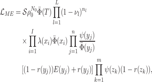
Abstract

Birth–death stochastic processes are the foundations of many phylogenetic models and are widely used to make inferences about epidemiological and macroevolutionary dynamics. There are a large number of birth–death model variants that have been developed; these impose different assumptions about the temporal dynamics of the parameters and about the sampling process. As each of these variants was individually derived, it has been difficult to understand the relationships between them as well as their precise biological and mathematical assumptions. Without a common mathematical foundation, deriving new models is nontrivial. Here, we unify these models into a single framework, prove that many previously developed epidemiological and macroevolutionary models are all special cases of a more general model, and illustrate the connections between these variants. This unification includes both models where the process is the same for all lineages and those in which it varies across types. We also outline a straightforward procedure for deriving likelihood functions for arbitrarily complex birth–death(-sampling) models that will hopefully allow researchers to explore a wider array of scenarios than was previously possible. By rederiving existing single-type birth–death sampling models, we clarify and synthesize the range of explicit and implicit assumptions made by these models. [Birth–death processes; epidemiology; macroevolution; phylogenetics; statistical inference.]

Evolutionary, demographic, and epidemiological pro- cesses leave a footprint in the branch length distribution and topology of reconstructed phylogenetic trees. This insight has inspired a huge effort to extract information about these processes by fitting stochastic models. For example, in molecular epidemiology, researchers have leveraged the fact that for many viral pathogens, such as HIV and SARS-CoV-2, accumulate genetic diversity on the timescale of transmission (Drummond et al. 2003; Duffy et al. 2008). This genetic diversity can be used to reconstruct the evolutionary relationships between viral variants sampled from different hosts, which in turn can help elucidate the epidemiological dynamics of a pathogen over time (Grenfell et al. 2004; Volz 2012). Similarly, phylogenetic trees can provide unique insights into the temporal variation in speciation and extinction rates (Morlon 2014).

Phylogenetic branching models can be broadly grouped into two classes. The first, based on Kingman’s coalescent process (Kingman 1982), has been widely used to examine changes in the historical population size of pathogens (Pybus et al. 2000; Strimmer and Pybus 2001; Drummond et al. 2005; Volz et al. 2009). These coalescent methods have also been applied to reconstruct macroevolutionary dynamics (Morlon et al. 2010). Coalescent models are well suited for estimating deterministic population dynamics; however, fitting highly stochastic processes, such as the dynamics of an emerging pathogen, is computationally intensive and in some cases the assumptions of the coalescent may not be appropriate (Stadler et al. 2015; Boskova et al. 2014; Volz and Frost 2014). The second class of models, which are collectively referred to as birth–death-sampling (BDS) models (Kendall 1948; Maddison et al. 2007; Stadler 2009; Stadler 2010), is well suited for stochastic scenarios, and are thus becoming an increasingly favorable and popular alternative to coalescent models in epidemiology (Stadler et al. 2012) and have long been the foundation of most macroevolutionary studies—both for inferring speciation and extinction dynamics (Raup 1985; Nee et al. 1994) and for estimating divergence times (Gernhard 2008; Heath et al. 2014). As the name implies, the BDS process includes three types of events: birth (pathogen transmission between hosts, or speciation in a macroevolutionary context), death (host death or recovery, or extinction in macroevolution), and sampling (including fossil collection in macroevolution).

In the context of epidemiology, BDS models have the additional property that the model parameters, which can be estimated from viral sequence data, explicitly correspond to parameters in classic structured epidemiological models that are often fit to case surveillance data. If we reparameterize these models, we can describe the dynamics of the basic and effective reproductive ratios ( and , respectively) over time (Stadler et al. 2012; Stadler et al. 2013) (see Box 1). A common research aim is to describe how the frequency of birth, death, and sampling events, and other derived variables such as , change throughout the course of an epidemic. There has been less work in macroevolution linking the parameters of a BDS model to those of an underlying more mechanistic model (but see Ezard et al. 2016) but this seems like a promising avenue for future development. As we detail below and in the Supplementary material available at Dryad at https://doi.org/10.5281/zenodo.5028470, there has been an astounding rise in the variety and complexity of BDS model variants. A key assumption in the specification of BDS submodels is whether all lineages alive at some time point are exchangeable (Stadler 2013) (such models are hereafter “single-type” models), meaning they diversify according to the same process, or if rather the diversification process is variable (“multitype” models; e.g., Maddison et al. 2007; FitzJohn 2012; Stadler and Bonhoeffer 2013; Rasmussen and Stadler 2019; Barido-Sottani et al. 2018), with lineages belonging to one of multiple possible states each characterized by a unique process. Each of these diversification processes can then be characterized by different dynamical assumptions. In the epidemiological case, these assumptions specify, for example, the nature of viral transmission and the sampling procedure (Stadler et al. 2013; Kühnert et al. 2014; Gavryushkina et al. 2014). While typically not explicitly tied to mechanistic evolutionary processes, there are a similar abundance of dynamical assumptions employed in the macroevolutionary context specifying the nature of biodiversity change through time (Nee 2006; Gernhard 2008; Morlon et al. 2011; Stadler 2011; Morlon 2014; Heath et al. 2014; Louca 2020).

Box 1: The Connection between BDS and SIR Models

The single-type BDS model is intimately related to the SIR compartmental model used in classic theoretical epidemiology. This connection illustrates the explicit and implicit assumptions of the general BDS model and its sub models. Here, we define the SIR epidemiological model, discuss how it can inform and be informed by these diversification models, and examine the shared assumptions of the two frameworks.

The SIR Model

The SIR model partitions the host population via infection status into susceptible (S), infected (I), and recovered (R) hosts. Infection of susceptible hosts occurs at a per-capita rate . Infected hosts may recover (at rate ), die of virulent cases (at rate ), or be sampled (at rate ). The cumulative number of sampled hosts is represented in the SIR model (Figure B.1 top) by . Upon sampling, infected hosts may be treated and hence effectively recover with probability . Hosts that have recovered from infection exhibit temporary immunity to future infection which wanes at rate . The special case of the SIR model with no immunity (the SIS model) is obtained in the limit as . In addition to these epidemiological processes, the SIR model includes demographic processes, such as host birth (rate ) and death from natural causes (rate ). While not shown explicitly in the figure, these epidemiological and demographic rates may change over time as a result of host behavioral change, pharmaceutical and nonpharmaceutical interventions, or host/pathogen evolution.

The BDS Model

The BDS model follows the number of sampled and unsampled viral lineages over time, analogous to the and classes of the SIR model. A key element of general BDS model is that birth and death rates may vary over time. This time dependence may be either continuous (Morlon et al. 2011; Rabosky and Lovette 2008b) or discrete (Stadler 2011; Stadler and Bonhoeffer 2013; Gavryushkina et al. 2014; Kühnert et al. 2014) Although arbitrarily time-dependent, the birth, death, and sampling rates in the general BDS model are assumed to be diversity-independent, analogous to the assumption of density-dependent transmission (pseudo mass action) in the SIR model (Keeling and Rohani 2008). Incorporating such diversity dependence into macroevolutionary models has been shown to increase the accuracy of extinction rate estimates and are necessary to accurately capture the saturation of diversity (Etienne et al. 2012). While some forms of diversity-dependence in diversification rates may be incorporated implicitly capturing deterministic diversity dependence as time dependence (Rabosky and Lovette 2008a), stochastic diversity-dependence (Etienne and Rosindell 2012) goes beyond the scope of the BDS models considered here.

The single-type BDS model assumes all viral lineages are exchangeable—this has several implications. First, all viral lineages are epidemiologically identical hence all mutations between them are neutral. Incorporating nonneutral genetic variation requires a multitype approach as in Equation (16). Second, transmission is independent of lineage age. In the macroevolutionary case, such age-dependence has been suggested to reflect niche differentiation in novel species (Hagen et al. 2015) and in the epidemiological case may reflect adaptation towards increased transmissibility following a host species-jumping event. Third, lineage exchangeability is reflected in the absence of an exposed (E) class in the SIR model in which hosts can, for example, transmit infections but not be sampled or vice versa. Finally, the single-type BDS model assumes all lineages are sampled at random and does not include submodels with nonrandom representation of lineages (Stadler et al. 2012).

Model Connections

Given their shared model assumptions, the single-type BDS model can be constrained explicitly to reflect an underlying SIR epidemic by setting the viral birth rate equal to the per-capita transmission rate of the infectious class and the viral death rate to the infectious recovery or removal rate , whereas the sampling rate is identical across models (Figure B1a). While constraining the birth, death, and sampling rates in this manner can be used to parameterize compartmental models (Kühnert et al. 2014) doing so is an approximation assuming independence between the exact timing of transmission, recovery or removal from the population, and sampling events in the SIR model and birth, death, and sampling events in the diversification model. The resulting tree likelihood in terms of the compartmental model is given by:

(B1)

While they are not submodels of the general BDS process given by equation 13, likelihood models have been developed that capture the full nonindependence of viral diversification and epidemiological dynamics for the SIR model specifically (Leventhal et al. 2012) and in compartmental models in general (Vaughan et al. 2019). The connection between the BDS process and SIR epidemiological models can also be used after the diversification rates are inferred to estimate the basic and effective reproductive rates (Stadler et al. 2012; Stadler and Bonhoeffer 2013). Specifically, the effective reproductive rate at time before the present day is given by . Although the SIR model is a useful epidemiological model for is simplicity, realistically modeling epidemic dynamics requires far more complex compartmental models. As reflected by their shared structure, the application of the single-type BDS model is restricted, however, to the assumptions of the SIR model alone and further methodological advances in multitype modeling are necessary for direct inference for the larger class of epidemiological models.

This flourishing of methods and models has facilitated critical insights into epidemics (du Plessis and Stadler 2015; Joy et al. 2016) and the origins of contemporary biodiversity (Morlon 2014; Schluter and Pennell 2017). However, this diversity of models has made it difficult to trace the connections between variants and to understand the precise epidemiological, evolutionary, and sampling processes that differ between them. Furthermore, despite their apparent similarities, these models have been derived on a case-by-case basis using different notation and techniques; this creates a substantial barrier for researchers working to develop novel models for new situations. And critically, it is imperative that we understand the general properties of BDS phylogenetic models and the limits of inferences from them (Louca and Pennell 2020a; Louca et al. 2021), and this is difficult to do without considering the full breadth of possible scenarios. Here, we address all of these challenges by unifying the whole class of phylogenetic BDS models. We do so by first deriving a likelihood for general single- and multitype BDS models; in the general case, we do not assume anything about the functional forms (i.e., temporal dynamics) of the various parameters including the sampling rate through time, the possibility of sampling ancestors (or not), or how the process was conditioned. While such general models may be useful for studying the mathematical properties of BDS models as a whole (Lambert and Stadler 2013; Louca and Pennell 2020a; Louca et al. 2021), statistical inference from these models requires researchers to make further constraints on the process. We prove that existing BDS model variants are indeed submodels of the more general case—and thereby clarify the specific assumptions made by different models—and provide a standardized notation and technique for deriving these and other submodels that have not previously been considered in the literature.

 

The Single-type Birth–Death-Sampling Model

Model specification

The BDS stochastic process begins with a single lineage at time before the present day. We note that this may be considerably older than the age of the most recent common ancestor of an observed sample which is given by . While we focus primarily on applications to epidemiology, our approach is agnostic to whether the rates are interpreted as describing pathogen transmission or macroevolutionary diversification.

In the model, transmission/speciation results in the birth of a lineage and occurs at rate , where () is measured in units of time before the present day (), such that can be time-dependent. We make the common assumption that lineages in the viral phylogeny coalesce exactly at transmission events, thus ignoring the within-host coalescent processes in the donor (Romero-Severson et al. 2016). Throughout, we will use as a a general time variable and to denote the time at which a specific event occurs as measured in units of time before the present day (see Supplementary Table S1). Lineage extinction, resulting from host recovery or death in the epidemiological case or the death of all individuals in a population in the macroevolutionary case, occurs at time-dependent rate . We allow for two distinct types of sampling: lineages are either sampled according to a Poisson process through time or binomially at very short intervals, which we term “concerted sampling attempts” (CSAs), where lineages at some specified time are sampled with probability ( denotes a vector of concerted sampling events at different time points). In macroevolutionary studies based only on extant lineages, there is no Poissonian sampling, but a CSA at the present (). In epidemiology, CSAs correspond to large-scale testing efforts (relative to the background rate of testing) in a short amount of time (relative to the rates of viral sequence divergence); for full explanation, see Appendix. We call these attempts rather than events because if is small or the infection is rare in the population, few or no samples may be obtained. CSAs can also be incorporated into the model by including infinitesimally short spikes in the sampling rate (more precisely, appropriately scaled Dirac distributions). Hence, for simplicity, in the main text we focus on the seemingly simpler case of pure Poissonian sampling through time except at the present-day, where we allow for a CSA to facilitate comparisons with macroevolutionary models; the resulting formulas can then be used to derive a likelihood formula for the case where past CSAs are included (see Appendix).

In the epidemiological case, sampling may be concurrent (or not) with host treatment or behavioral changes resulting in the effective extinction of the viral lineage. Hence, we assume that sampling results in the immediate extinction of the lineage with probability . As with the CSAs, this arbitrary time dependence allows for the incorporation of Dirac spikes in any of these variables, for example, with mass extinctions () and lagerstätten in the fossil record () (Magee and Höhna 2021). Similarly, in the case of past CSAs, we must include the probability, , that sampled hosts are removed from the infectious pool during the CSA at time . Poissonian sampling without the removal of lineages () can be employed in the macroevolutionary case to explicitly model the collection of samples from the fossil record (such as the fossilized-birth–death process; Heath et al. 2014).

For our derivation, we make no assumption about the temporal dynamics of , , , or ; each may be constant, or vary according to any arbitrary function of time given that it is biologically valid (nonnegative and between 0 and 1 in the case of ). Specifically, the time-varying functions may be any piecewise-continuous functions of time with at most finite number of discontinuities (see Rate Assumption section in the Appendix). Note that these functions need not be differentiable. We make the standard assumption that at any given time any given lineage experiences a birth, death or sampling event independently of (and with the same probabilities as) all other lineages. We revisit this assumption in Box 1 where we discuss how the implicit assumptions of the single-type BDS process are well summarized by the diversification model’s relationship to the SIR epidemiological model. Our resulting general time-variable BDS process can be fully defined by the parameter set .

In order to make inference about the model parameters, we need to calculate the likelihood, , that an observed phylogeny, , is the result of a given BDS process. With respect to the BDS process there are two ways to represent the information contained in the phylogeny , both of which have been used in the literature, which we call the “edge” and “critical time” representations, respectively. We begin by deriving the likelihood in terms of the edge representation and later demonstrate how to reformulate the likelihood in terms of critical times. In the edge representation, the phylogeny is summarized as a set of edges in the mathematical graph that makes up the phylogeny, numbered 1–11 in Figure B.1c, and the types of events that occurred at each node. We define as the probability that the edge which begins at time and ends at time gives rise to the subsequently observed phylogeny between time and the present day. The likelihood of the model for the observed tree is then, is by definition : the probability density that the stem lineage ( in Figure B.1c) gives rise to the observed phylogeny from the origin, , to the present day. We find that it is more intuitive to derive the likelihood in terms of the edge representation, as we show below; from this it is straightforward to derive the critical times formulation which results in mathematical simplification. Below, we present our five-step technique for the derivation of the tree likelihood.

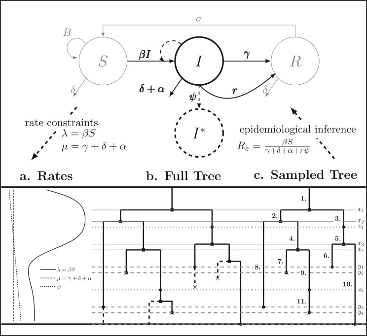
Figure B.1.

BDS-SIR model connection. Top: The SIR epidemiological model. Black (gray) lines and classes represent rates and variables followed (in)directly by the BDS model. The SIR model can be used to constrain the rates of the BDS model (a). Simulated forward in time, the result of the BDS stochastic processes is a full tree (b) giving the complete genealogy of the viral population. Pruning away extinct and unsampled lineages produces the sampled tree (c). Arising from a BDS process, this sampled tree can be summarized in two ways. First by the set of edges (labeled 1–11) or as a set of critical times (horizontal lines) including: 1) the time of birth events (solid, ) 2) terminal sampling times (dashed, ), and 3) ancestral sampling times (dotted, ). Given the inferred rates from a reconstructed sampled tree, these rates can be used to estimate characteristic parameters of the SIR model, for example, the basic or effective reproductive number.

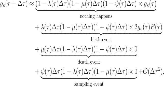
Step 1. Deriving the Initial Value Problem (IVP) for

We derive the IVP for the likelihood density using an approach first developed by (Maddison et al., 2007). We begin by deriving the recursion equation for by considering all the possible events that could occur along edge between time and assuming that that is small enough such that at most one event is likely to occur.

(1)

Here, is the probability that a lineage alive at time leaves no sampled descendants at the present day. We will examine this probability in more detail below. Assuming is small, we can approximate the above recursion equation as the following difference equation.

(2)

By the definition of the derivative, we have:

(3)

Equation (3) is known as the Kolmogorov backward equation of the BDS process (Feller 1949; Louca and Pennell 2020b). Beginning at time , the initial condition of depends on which event occurred at the beginning of edge .

(4)

Together Equations (3) and (4) define the initial value problem for as a function of the probability .

Because the likelihood density is the solution to a linear differential equation with initial condition at time , we can express its solution as follows:

(5)

where the auxiliary function, , is given by:

(6)

This function, , maps the value of at time to its value at , and hence is known as the probability “flow” of the Kolmogorov backward equation (Louca and Pennell 2020b).

Step 2. Deriving the IVP for

We derive the IVP for in a similar manner as above, beginning with a difference equation.

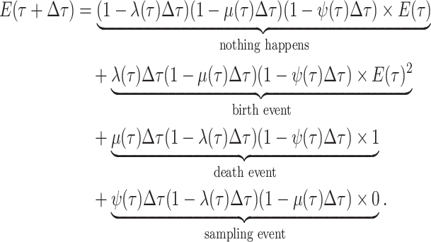(7)

By the definition of a derivative, we have:

(8)

where is the probability a lineage is sampled at the present day. The initial condition at time is therefore the probability that a lineage alive at the present day is not sampled. Given an analytical or numerical general solution to , we can find the likelihood by evaluating , as follows.

Step 3. Deriving the expression for .

Given the linear nature of the differential equation for and hence the representation in Equation (5)), the likelihood is given by the product over all the initial conditions times the product over the probability flow for each edge.

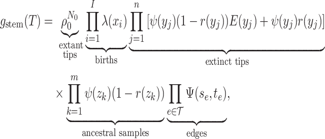(9)

where , , and are the times at which individual birth, terminal sampling and ancestral sampling events occur as we elaborated below.

Step 4. Representing in terms of critical times.

Equation (9) can be further simplified by removing the need to enumerate over all the edges of the phylogeny (the last term of Equation (9)) and writing in terms of the tree’s critical times (horizontal lines in Fig. B.1). The critical times of the tree are made up of three vectors, , , and , as well as the time of origin . The vector gives the time of each birth event in the phylogeny and has length where is the number of lineages sampled at the present day and is the number of terminal samples. Unless noted otherwise the elements of vector are listed in decreasing order, such that and hence is the time of the most recent common ancestor . The vector gives the timing of each terminal sample and hence has length whereas vector gives the timing of each ancestral sample and has length . With respect to the BDS likelihood then the sampled tree is summarized by . We note that the critical times only contain the same information as the edges as a result of the assumptions of the BDS process but are not generally equivalent representations of .

As a result of the linear nature of it is straightforward to rewrite the likelihood in Equation (9) in terms of the critical-time representation of the sampled tree. Defining

(10)

the probability flow can be rewritten as the following ratio:

(11)

This relationship allows us to rewrite the likelihood by expressing the product over the edges as two separate products, one over the start of each edge and the other over the end of each edge which in turn allows us to rearrange and cancel terms to obtain an alternative likelihood expression. Edges begin (value of ) at either: 1) the tree origin, 2) a birth event resulting to two lineages, or 3) an ancestral sampling event. Edges end (values of ) at either: 1) a birth event, 2) an ancestral sampling event, 3) a terminal sampling event, or 4) the present day. 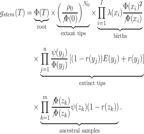Hence we have:

(12)

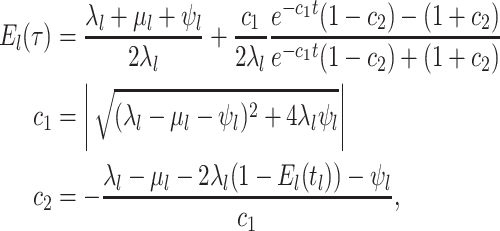
Note . While Equations (9) and (12) are numerically identical, the critical time expression is more convenient for application as it requires numerically evaluating only a single function as given by Equation (10).

Step 5. Conditioning the likelihood

While Equation (12) is equal to the basic model likelihood for the phylogeny , it is often appropriate to condition the tree likelihood on the tree exhibiting some property, for example the condition there being at least sampled lineage. Imposing a condition on the likelihood is done by multiplying by a factor . Various conditioning schemes are considered in section A4 and listed in Table S3 with the value of ranging in complexity from a constant to a general function of the model parameters. The resulting likelihood expression for the general BDS model is:

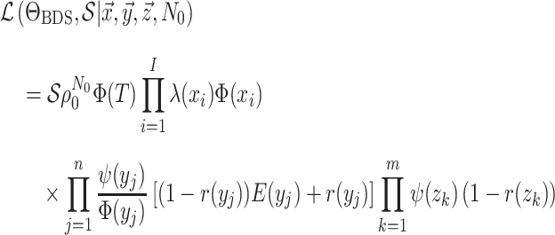(13)

Many Existing Models are Special Cases of this General BDS Model

A large variety of previously published BDS models in epidemiology and macroevolution are special cases of the general model presented here (for a summary of the models we investigated, see Supplementary Table S2. Indeed, we can obtain the likelihood of these models by adding mathematical constraints (i.e., simplifying assumptions) to the terms in Equation (13). Our work thus not only provides a consistent notation for unifying a multitude of seemingly disparate models, it also provides a concrete and numerically straightforward recipe for computing their likelihood functions. We recognize that there are many valid approaches for deriving tree likelihoods for BDS models with share many similarities with our own (e.g., Nee et al. 1994; Maddison et al. 2007; Gernhard 2008; Morlon et al. 2011; Lambert and Stadler 2013; Lambert 2018; Laudanno et al. 2020; Louca and Pennell 2020b) and do not claim ours is superior to these; however, we have found our technique to be intuitive and flexible. We have implemented the single-type BDS likelihood in the R package (Louca and Doebeli 2018), including routines for maximum-likelihood fitting of BDS models with arbitrary functional forms of the parameters given a phylogeny and routines for simulating phylogenies under the general BDS models (functions , and ).

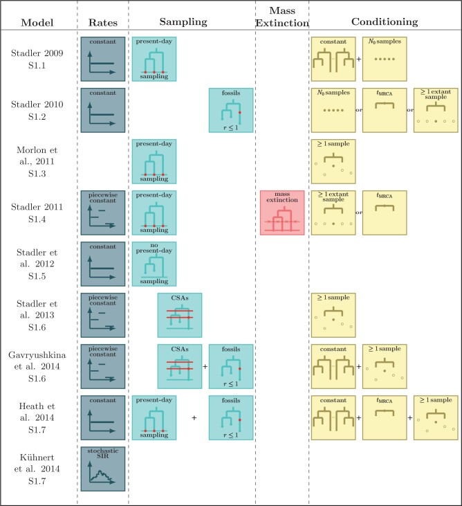
Figure 1 summarizes the simplifying assumptions that underlie common previously published BDS models; these assumptions generally fall into four categories: 1) assumptions about the functional form of birth, death, and sampling rates over time, 2) assumptions pertaining to the sampling of lineages, 3) the presence of mass-extinction events, and 4) the nature of the tree-conditioning as given by . Here, we provide a brief overview of the type of previously invoked constraints which are consistent (or not) with our unified framework; for full details on each specific case, we refer readers to the Supplementary material. While we illustrate these constraints within the single-type context, analogous assumptions can be made within the multitype context examined in the following section.

Figure 1.

Submodel assumptions. Rate, sampling, mass extinction, and conditioning assumptions of existing submodels of the general time-variable BDS process. The key points are that i) each of the previously developed models we considered can be obtained by adding specific combinations of constraints to the various parameters of the general BDS model; and ii) that there are many plausible, and potentially biologically informative combinations of constraints that have not been considered by researchers in epidemiology or macroevolution.

In regards to rate assumptions, many early BDS models (Stadler 2009; Stadler 2010; Stadler et al. 2012) assumed that the birth, death, and sampling rates remained constant over time. This is mathematically and computationally convenient since an analytical solution can easily be obtained for . In the epidemiological case, holding constant, however, implies that the number of susceptible hosts is effectively constant throughout the epidemic and/or that the population does not change its behavior over time; this is an unrealistic assumption given seasonal changes or changes in response to the disease itself. As such, this assumption is only really valid for small time periods or the early stages of an epidemic. This is useful for estimating the basic reproductive number, , of the SIR model (Box 1) but not for the effective reproductive number at later time points (Stadler et al. 2012).

A similarly tractable, but more epidemiologically relevant, model is known as the “birth–death-skyline” variant (Stadler and Bonhoeffer, 2013; Gavryushkina et al., 2014), in which rates are piecewise-constant functions through time (like the constant rate model, there is also an analytical way to calculate the likelihood of this model; see Appendix). The BDS skyline model has been implemented under a variety of additional assumptions in the Bayesian phylogenetics software BEAST2 (Bouckaert et al. 2019). The BDS skyline model has also been extended by (Kühnert et al., 2014) to infer the the parameters of an underlying stochastic SIR model. In this case the diversification model parameters are random variables that emerge from stochastic realizations of the epidemiological model given by , see Equation (B1). Finally, the birth–death skyline model with piecewise constant rates can also be applied in the macroevolutionary case when no sampling occurs through time, (Stadler 2011).

In addition to imposing constraints on the temporal variation in the rates, previously derived submodels have considered a variety of different assumptions about the nature of the sampling process. Most notably, in macroevolutionary studies, sampling of molecular data typically occurs only at the present day (Stadler 2009; Stadler 2011; Morlon et al. 2011) whereas past Poissonian sampling can be introduced to include the sampling of fossil data (Heath et al. 2014). In epidemiology, concerted sampling at the present day is likely biologically unrealistic (Stadler et al. 2012), though in some implementations of the models, such a sampling scheme has been imposed. These concerted sampling attempts prior to the present day as well as mass extinction events can be incorporated via the inclusion of Dirac distributions in the sampling and death rates, respectively. Finally, previous models often multiply the likelihood by a factor in order to condition on a particular observation (e.g., observing at least one lineage or exactly lineages), enumerate indistinguishable trees (e.g., accounting for possible orientations or unlabeled trees) (Gavryushkina et al. 2013; Gavryushkina et al. 2014; Stadler 2009), or to reflect known uncertainties. The “fossilized-birth–death” likelihood derived by Heath et al. (2014) for example, includes a factor that reflects the uncertainty in the attachment and placement of fossils on the macroevolutionary tree. This fossilized-birth–death process has been used to estimate divergence times and to model lineage diversification (Gavryushkina et al. 2017; Landis et al. 2021). Variants of the fossilized-birth–death process, for example including mass extinction events, are feasible and can be derived using our approach. We also note that models similar to the time-variable fossilized-birth–death process have been developed for cases when phylogenetic data is not available (i.e., when only including fossil occurrence data; see Silvestro et al. 2014; Lehtonen et al. 2017); we have not investigated how these models relate to our generalized BDS model but we speculate that it would be possible to also bring these models into a common framework with those that we have discussed. Supplementary material demonstrates how these submodels can be re-derived by either imposing the necessary constraints on the general likelihood formula given in Equation (13) or, alternatively, by starting from the combinations of assumptions and using the five-step procedure outlined above.

The Multitype Birth–Death-Sampling Model

A common extension of the single-type diversification models explored above is to consider cases where the diversification rates () and probabilities () vary among lineages as a function of a categorical “lineage type”. This lineage type can be defined in terms of specific (Maddison et al. 2007; Rasmussen and Stadler 2019) or unspecified traits (Beaulieu and O’Meara 2016) or trait combinations (FitzJohn 2012) (for reviews of these models see Morlon 2014; Ng and Smith 2014). Representing these lineage types as colors at nodes and along branches of the tree, we first extend the single-type model above by deriving the likelihood of a fully colored tree with topology where the states along all edges of the phylogeny are known as given by . The resulting likelihood is an extension of the likelihood first developed by Barido-Sottani et al. (2018), where the diversification rates and probabilities are allowed to vary arbitrarily through time. To illustrate that our derivation is indeed quite general, we follow the model developed (independently) by Magnuson-Ford and Otto (2012) and Goldberg and Igić (2012), where the state of lineages can change either anagenetically, with a lineage of type mutating to a type at rate or cladogenetically, with a lineage of type giving rise to a daughter lineage of type at rate . Lineages go extinct at a state-dependent rate and are sampled at rate . As in the single-type model, upon sampling lineages are removed from the population with probability whereas all lineages alive at the present day are sampled with a probability . As discussed in depth by Goldberg and Igić (2012), the other discrete variations of state-dependent diversification models (FitzJohn et al. 2009; Goldberg et al. 2011; FitzJohn 2012) fall out as special cases of this model. (See Ng and Smith 2014; Caetano et al. 2018; Louca and Pennell 2020b for further discussion of the connection between multitype models.)

We use the five-step technique specified above for the single-type case to derive the probability of observing a given colored tree under a general multitype model (see Supplementary material II). We first derive the initial value problem for the probability that an edge of type in the tree at time gives rise to the subsequently observed phylogeny. The edge here refers not to an edge in the topological tree, but to a segment of the tree all of one state between birth, sampling, or mutation events.

(14)

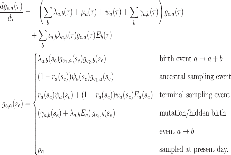
Equation (16) distinguishes between multiple types of birth events as pictured in Supplementary Figure S1. Birth events may be symmetric, with both daughter lineages inheriting the parental type. The exchangeability of the resulting daughter lineages is reflected in the indicator variable which takes on value of 2 if and 1 otherwise. In contrast asymmetric birth events the resulting daughter lineages differ in type due to caldogenetic change. Importantly, the differential equation for is linear and hence has a known general solution . As in the single-type model is the probability flow (Louca and Pennell 2020b) mapping the probability from the initial state at time to the probability at time .

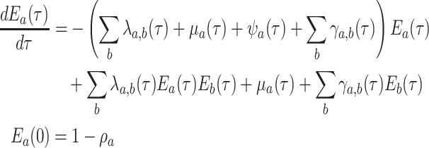
An analogous initial value problem can be derived for the probability , that a lineage of type alive at time leaves no observed descendants in the sampled tree.

(15)

This is a nonlinear differential equation and must be solved numerically. Given the solution of and the likelihood for the fully colored tree is characterized by a series of critical times: first, the times at which a lineage of type gives birth to a lineage of type , the ages of tip samples of type , the ages of ancestral samples of type , and the times at which lineages are observed to transition events from type to type . The resulting likelihood is given by:

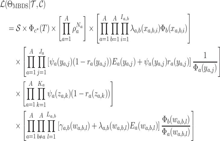(16)

Here, is an arbitrary form of conditioning as in Equation (13) and , a complete list of notation is given in Table S4.

Equation (16) gives the likelihood of a fully colored tree, the tree topology plus the state along each branch and at each node in the tree. This likelihood is a generalization of that presented by (Barido-Sottani et al., 2018, 2020). Maximizing Equation (16) while incrementally adding and removing changes in state along the branches of the tree can be used to identify clades with distinct diversification parameters. This method can be used, for example, to identify transmission clusters within a disease outbreak (Barido-Sottani et al. 2018). This likelihood is distinct from but related to post-traversal likelihood methods developed to infer state-dependent diversification rates given the known state of sampled lineages (e.g., Maddison et al. 2007; Magnuson-Ford and Otto 2012; Stadler and Bonhoeffer 2013). Specifically, these methods give the likelihood where is the state of present-day, , past , and ancestral, , sampled lineages. The relationship between the numerically obtained post-traversal likelihood and the closed-form fully colored likelihood (Equation (16)) is given by:

(17)

Here, is one specific coloring of the tree (e.g., a maximum parsimony ancestral state reconstruction) that is consistent with the observed states. We include Equation (17) as it clarifies the relationship between these two different approaches that have been used to calculate multitype likelihoods in phylogenetics. Whether or not this is useful for inference is an open question as is challenging to compute (the details of which are beyond the scope of the present paper).

Concluding Remarks

In this article, we have unified a broad class of BDS models that have been widely used both in epidemiology and macroevolution. And in doing so, we have also presented a standardized notation and approach that can be used both for deriving the various submodels that have previously been studied as well as novel combinations of assumptions about the model parameters. The unification of these models clarifies the connections between BDS variants, facilitates the development of new variants tailored to specific scenarios, and provides a structure for understanding how results depend on model assumptions (Kirkpatrick et al. 2002; Lafferty et al. 2015; Louca and Pennell 2020a). And importantly, given the recent discovery of widespread nonidentifiability in birth–death processes fit to extant-only (Louca and Pennell 2020a) and serially sampled (Louca et al. 2021) phylogenetic data, there is a critical need to explore a much broader range of BDS models than were previously considered and the mathematical generalization presented here will be enable this.

Appendix: Adding assumptions to the general model

In this appendix, we demonstrate how one can obtain the likelihood of submodels with different sets of assumptions by applying constraints to the general likelihood. There are four classes of assumptions that are commonly applied in epidemiological and macroevolutionary studies. First, researchers can make assumptions about the functional form of the birth, death, and sampling rates. Here, we address two such unique assumptions: i) birth, death, and sampling rates are constant (see the Rate Assumptions section, Sections S1.1, S1.2, and S1.5 of the Supplementary material; and ii) birth, death, and sampling rates are piecewise-constant functions of time (see Piecewise-constant Rates section, Section S1.6 of the Supplementary material). The cases where birth, death, and sampling rates are defined by a stochastic or deterministic SIR model are mathematically analogous to the cases of the piecewise-constant and general time-variable models respectively. All additional constraints imposed will depend on the exact compartmental model used and hence we will not discuss them in detail in this section. The second major class of assumptions pertains to sampling. There are four such sampling assumptions: i) sampling happens only at the present day as in a birth–death model (see No Sampling at the Present Section, Sections S1.1, S1.3, and S1.4 of the Supplementary material) or as implemented in the “Birth Death Skyline Contemporary” prior in the BDSKY package in BEAST2; ii) the absence of concerted present-day sampling (see Birth–Death Models section, Section S1.5 of the Supplementary material); iii) the inclusion of ancestral samples with sampled descendants (Sections S1.6 and S1.7 of the Supplementary material; and iv) concerted sampling attempts (CSA) during which all lineages are sampled with a given probability (see Concerted Sampling Attempts section, Section S1.6 of the Supplementary material). The third assumption class considers the presence of mass extinction events (see Mass Extinction section, Section S1.5 of the Supplementary material). The fourth and final major class of assumptions deal with the conditioning of the likelihood. The various conditioning schemes are explored in below and summarized in Supplementary Table S3 available on Dryad.

 

Rate Assumptions

Constant Rates

• Model assumptions: Constant diversification rates: , , , and constant removal probability .

• The IVP for ):  

  
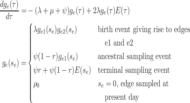
• The IVP for :  

  
  In this case the IVP for is a Bernoulli differential equation and has a known analytical solution. As given by Equation 1 in (Stadler, 2010) this solution is given by:

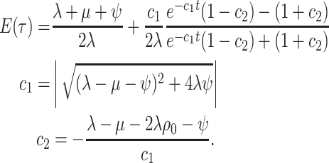
  (A1)
• The probability flow:  

  
• The likelihood:  

  (A2)

Piecewise-Constant Rates

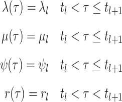
• Model assumptions: Divide time into intervals defined by transition times  . Define rates and removal probabilities constant within a given interval.

  

• The IVP and solution for : Given the definitions of , , , and within each time interval the IVP for is identical to that given in Equations (3) and (4). If is the probability density within time interval than .

• The IVP and solution for : As with , the IVP for is given by Equation (8). With the piecewise-constant rate assumptions, however, the general solution for between is known (similar to Equation (A1)). Defining and we have:

  

  where for and .

• The probability flow: We define a probability subflow within each time interval. Specifically, in the th time interval.

  
  The complete flow can be expressed as a function of the subflows in the following manner:

  (A3)

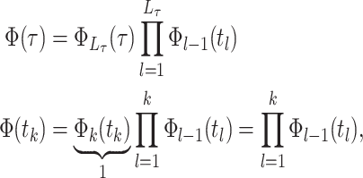
  where is the index of the time at or after time , that is, the largest index such that .

• The likelihood: Given these piecewise definitions we substitute them into the general BDS likelihood (13).

  

  where we use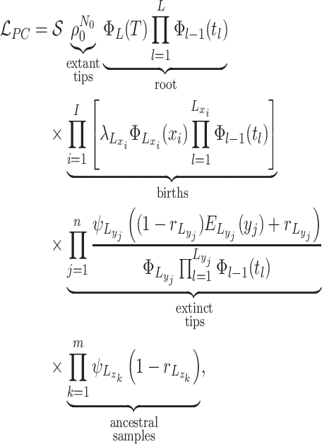 to denote the piecewise-constant assumption.

  We can simplify several of these products. Let be the number of birth events and the number of sampling events .

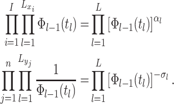
  (A4)
  Let be the number of observed lineages alive at time . Because the number of observed lineages increases with each birth and decreases with each sampled tip, counting the root we have . Substituting the expressions for the into the likelihood and using the definition of we have:

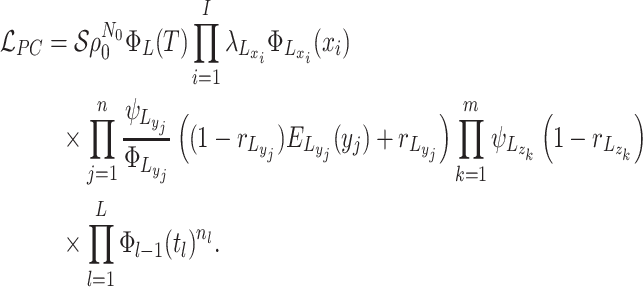
  (A5)

Sampling Assumptions

Birth–Death Models

• Model assumptions: The birth–death model assumes that . Note that the probability of sampling a lineage given it is alive at the present day remains as (incomplete sampling).

• IVP for :  

  
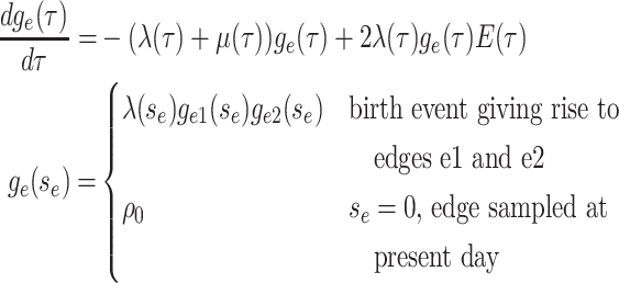
• IVP for :  

  
  Note in this case equals , the probability a lineage leaves no sampled extant descendants. As demonstrated by (Morlon et al., 2011) there exists a general solution to this initial value problem, see Section ?? for more details. This general solution is given by:

  
• The probability flow: From (Morlon et al., 2011), the probability flow can be written as the following:

  
• The likelihood:  

  (A6)

No Sampling at the Present

Here, we consider the case when . The likelihood follows exactly as in the general model case. The resulting likelihood expression is given by:

(A7)

Note that in this case .

Concerted Sampling Attempts

• Model assumptions: Here, we introduce concerted sampling attempts (CSA) at known points in time, . Like the CSA at the present day, and in contrast to the background Poissonian sampling rate, during the CSA at time every lineages is sampled with a fixed probability . In the derivation of the likelihood below, we must distinguish between three different sampling event types. First, past Poissonian sampling events are those that do not occur during CSAs. Second, past concerted sampling events are those that occur during a CSA at time . Finally, present concerted sampling events are those that occur at the present day . Past concerted sampling attempts can be included in the general model above by adding Dirac distributions to the Poisson sampling rate function. Namely,

  (A8)

  where is the background Poissonian sampling rate and . The definition of comes from solving the CDF of the exponentially distribution for the “effective sampling rate” such that the probability of a lineage being sampled is .
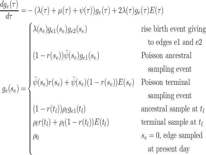
• IVP for :  

  

  The solution to is given by Equations (5) and (6).

• IVP for : As with , the IVP for is identical to that given for the general model in Equation (8). Except in rare cases the IVP must be solved numerically hence requiring numerical integration over Dirac distributions which can prove to be problematic.

  Note however, that when examining the integrals over the CSAs, a priori, it is a matter of convention whether the Dirac distribution should be considered as “integrated over” when located at the upper integration bound or at the lower integration bound . Whichever convention we chose, we must rigorously obey it so that the ratio correctly evaluates to whenever . Using the former convention, we can rewrite the probability at each concerted sampling time as:

  

  where denotes the limit as time approaches from below. Hence, the probability at any time can be evaluated numerically by considering the dynamics between successive CSAs and at each CSA separately.
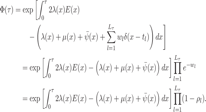
• The probability flow: The probability flow is given by:

  

  As with integration over the dirac distributions can be problematic and hence we rewrite this expression separating out these terms. Let be the oldest CSA occurring at or after time , that is, the largest index for which .

  (A9)
  We define:

  (A10)

  which means that we can rewrite Equation (A9) as:

  (A11)
• The likelihood: The edge representation of is given by:

  
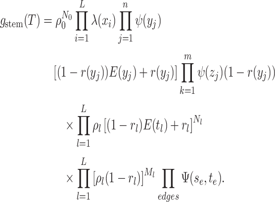  The critical time representation of is given by:

  

   

  

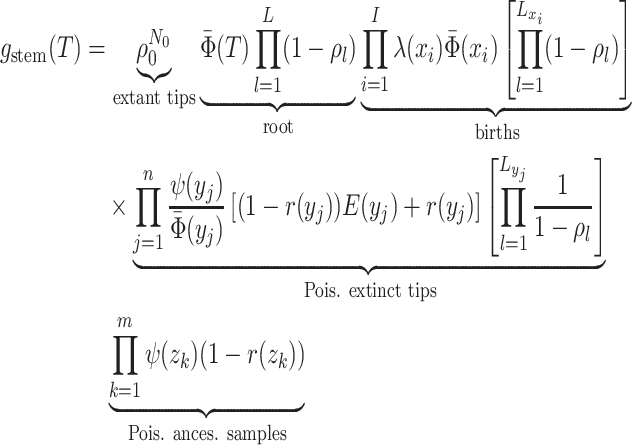
  where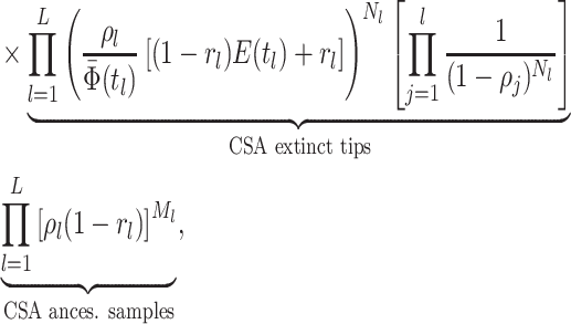 is the number of tip samples (samples without descendants) obtained during the th CSA and is the number of ancestral samples (sequences with descendants). By changing how we enumerate birth, death, and sampling events we can greatly simplify this likelihood. First, let be the number of branching events at or before the th CSA. In other words, is the number of branching events if the tree were trimmed at the th CSA. Then:

  (A12)
  Second, let be the number of past Poissonian sampling events before time . Then:

  (A13)
  Finally, let be the number of past lineages sampled during a CSA at or before the CSA at time . Hence, . Then:

  (A14)
  The likelihood hence simplifies to: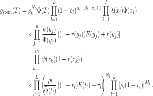

  

  Let be the number of lineages that cross , that is, the number of lineages alive at time with sampled descendants at some younger age. Note that by this definition . Then is the number of tips in the tree had it been trimmed at age whereas is the number of branching events. Therefore we must have . This allows us to simplify the conditioned likelihood given below.

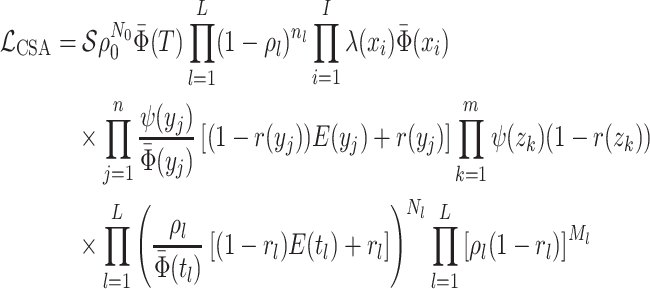
  (A15)

Mass Extinction

• Model assumptions: In addition to the Poisson birth death and sampling events considered in the general model, there are mass extinctions events occurring at times . During the th mass extinction event each lineage goes extinct with probability . As with concerted sampling such mass extinction events can be introduced into the model by adding a set of dirac-delta functions to the Poisson death rate, .

  (A16)

  where .

• IVP for : The initial value problem for is identical to that given in equation by Equations (3) and (4) except that is now includes the mass extinction events.

• IVP for : The IVP for to that given by Equation (8) except where the extinction rate is given by Equation (A16). The solution to is obtained by numerical integration. Given the dirac-delta functions this numerical integration can be carried out in a piecewise manner integrating separately between and over each mass extinction event. Defining as the solution up to but not including the mass extinction event at time , we have:

  

  The first term reflects the probability that a lineage that does not go extinct during the th mass extinction event leaves no observable offspring (with probability ) whereas the second term reflects the fact that all lineages that go extinct during the th mass extinction leave no observed descendants with probability 1.

• The probability flow: The solution to the IVP is once again given by where:

  

  As with the CSAs, let be the last index such that . We can separate out the mass extinction terms in the following way.

  

  where is defined as in Equation (A10).

• The likelihood: Given these initial value problems the likelihood follows as in the general model.

  
  As with the CSAs we can use relations analogous to Equations A12–A14 to rewrite the likelihood:

  (A17)

  where is defined as before as the number of lineages present at time .

Alternative Conditioning

Supplementary Table S3 lists a number of possible conditionings, that can be applied to the tree likelihood. First, is the trivial case of no conditioning which gives the probability of the observed tree including the stem edge between time and . To obtain the model likelihood excluding the stem edge, that is, conditioning of the , can be obtained by setting . Recall that the elements of are ordered such that is the first (oldest) birth event.

Acknowledging that one would not reconstruct a phylogeny without any sampled lineages, we can condition the likelihood on observing at least one sampled lineage (either at or before the present day) given the time of origin, . Or as with , conditioning on at least one sampled lineage given the . In order to have at least one sampled lineage and a most recent common ancestor, however, each daughter lineage of the common ancestor must have at least one descendent. Hence, we have . The general birth–death-sampling model assumes that all lineages alive at the present day are sampled with probability . As with concerted sampling attempts (CSAs) prior to the present day, this present day CSA may include the sampling of multiple lineages as well as possibly resulting in no sampled lineages. As with and we can condition the tree likelihood on observing at least one extant lineage at the present day. To do so, we define , the probability that a lineage alive at time has no extant descendants. Conditioning on the time of origin we have: . Conditioning on the time of the most recent common ancestor we have: , where now at least one of the two daughter lineages of the common ancestor has a present day sample. In many cases is modified, however, to condition on both daughter lineages having an extant sampled descendent: .

As an alternative to conditioning on at least one extant sampled descent, tree likelihoods can be conditioned on having exactly   sampled (extant) descendants. Let be the probability a lineage alive at time has exactly descendants. Although a general expression for is unknown, in the case of constant birth, death, and sampling rates (the case in which this form of conditioning has been applied), the expression for is given by (Gernhard, 2008), (Kendall, 1948) and Theorem 3.3 by (Stadler, 2010):

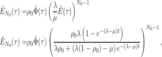where, like , is given by Equation (10) evaluated with where . Given the time of origin we can condition on observing exactly lineages by setting . When is given instead, then the number of descendants of the two daughter lineages must add up to while both daughter lineages must still have at least one descendant (see (Stadler, 2010) Corollary 3.9).

While early BDS models often employed such conditioning (Stadler 2009; Stadler 2010), this form of conditioning has not been employed in many later models perhaps because the biological justification for such conditioning is vague.

The final form of conditioning used in the literature, which we will represent simply as , is the multiplication of the BDS likelihood by a constant to account for the enumeration over the possible indistinguishable representations of a given tree. The value of this constant depends on whether the tree considered is “labeled” and “oriented” (Gavryushkina et al. 2013) and whether, as in the derivation here, the vector of birth events, , is (un)ordered. Inclusion of such a constant should have no effect on the maximum likelihood inference of the model parameters given a specified tree. In cases where the constant is a function of the critical times (Heath et al. 2014), it can influence the inference when the parameters and the tree are jointly estimated.

Supplementary Material

Data available from the Dryad Digital Repository: https://doi.org/10.5281/zenodo.5028470.

Funding

This work was supported by a Grant for Catalyzing Research Clusters awarded to the UBC Biodiversity Research Centre,NSF DEB Grant [#2028986 award to S.L. and M.W.P.]; a NSERC Discovery Grant to M.W.P.; and in part by the EEB department Postdoctoral Fellowship from the University of Toronto to A.M.; in part by a Canadian Institutes of Health Research (CIHR) doctoral award [#6557] to A.M.c.L..; a Genome Canada Bioinformatics and Computational Biology grant [287PHY], CIHR coronavirus rapid response program grant [440371] to J.B.J. and is grateful to the British Columbia Centre for Excellence in HIV/AIDS for additional funding support.

References

- Barido-Sottani J., Vaughan T.G., Stadler T. 2018. Detection of HIV transmission clusters from phylogenetic trees using a multi-state birth–death model. J. R. Soc. Interface 15:20180512. [DOI] [PMC free article] [PubMed] [Google Scholar]
- Barido-Sottani J., Vaughan T.G., Stadler, T. 2020. A multitype birth–death model for Bayesian inference of lineage-specific birth and death rates. Syst. Biol. 69:973–986. [DOI] [PMC free article] [PubMed] [Google Scholar]
- Beaulieu J.M., O’Meara B.C. 2016. Detecting hidden diversification shifts in models of trait-dependent speciation and extinction. Syst. Biol. 65:583–601. [DOI] [PubMed] [Google Scholar]
- Boskova V., Bonhoeffer S., Stadler T. 2014. Inference of epidemiological dynamics based on simulated phylogenies using birth-death and coalescent models. PLoS Comput. Biol. 10:1–18. [DOI] [PMC free article] [PubMed] [Google Scholar]
- Bouckaert R., Vaughan T.G., Barido-Sottani, J., Duchêne S., Fourment M., Gavryushkina A., Heled J., Jones G., Kühnert D., Maio N.D., Matschiner M., Mendes F.K., Müller N.F., Ogilvie H.A., du Plessis, Popinga A., Rambaut A., Rasmussen D., Siveroni I., Suchard M.A., Wu C.-H., Xie D., Zhang C., Stadler T., Drummond A.J. 2019. BEAST 2.5: an advanced software platform for Bayesian evolutionary analysis. PLoS Comput. Biol. 15:e1006650. [DOI] [PMC free article] [PubMed] [Google Scholar]
- Caetano D.S., O’Meara B.C., Beaulieu J.M. 2018. Hidden state models improve state-dependent diversification approaches, including biogeographical models. Evolution 72:2308–2324. [DOI] [PubMed] [Google Scholar]
- Drummond A.J., Pybus O.G., Rambaut A., Forsberg R., Rodrigo A.G. 2003. Measurably evolving populations. Trends Ecol. Evol. 18:481–488. [Google Scholar]
- Drummond A.J., Rambaut A., Shapiro B., Pybus O.G. 2005. Bayesian coalescent inference of past population dynamics from molecular sequences. Mol. Biol. Evol. 22:1185–1192. [DOI] [PubMed] [Google Scholar]
- du Plessis L., Stadler T. 2015. Getting to the root of epidemic spread with phylodynamic analysis of genomic data. Trends Microbiol. 23:383–386. [DOI] [PubMed] [Google Scholar]
- Duffy S., Shackelton L.A., Holmes E.C. 2008. Rates of evolutionary change in viruses: patterns and determinants. Nat. Rev. Genetics 9:267–276. [DOI] [PubMed] [Google Scholar]
- Etienne R.S., Haegeman B., Stadler T., Aze T., Pearson P.N., Purvis, A., Phillimore A.B. 2012. Diversity-dependence brings molecular phylogenies closer to agreement with the fossil record. Proc. R. Soc. B 279:1300–1309. [DOI] [PMC free article] [PubMed] [Google Scholar]
- Etienne R.S., Rosindell J. 2012. Prolonging the past counteracts the pull of the present: protracted speciation can explain observed slowdowns in diversification. Syst. Biol. 61:204–204. [DOI] [PMC free article] [PubMed] [Google Scholar]
- Ezard T.H.G., Quental T.B., Benton M.J. 2016. The challenges to inferring the regulators of biodiversity in deep time. Philos. Trans. R. Soc. B 371:20150216. [DOI] [PMC free article] [PubMed] [Google Scholar]
- Feller W. 1949. Proceedings of the [First] Berkeley Symposium on Mathematical Statistics and Probability. University of California Press, Berkeley California. [Google Scholar]
- FitzJohn R.G. 2012. Diversitree: comparative phylogenetic analyses of diversification in R. Methods Ecol. Evol. 3:1084–1092. [Google Scholar]
- FitzJohn R.G., Maddison W.P., Otto S.P. 2009. Estimating trait-dependent speciation and extinction rates from incompletely resolved phylogenies. Syst. Biol. 58:595–611. [DOI] [PubMed] [Google Scholar]
- Gavryushkina A., Heath T.A., Ksepka D.T., Stadler T., Welch D., Drummond A.J. 2017. Bayesian total-evidence dating reveals the recent crown radiation of penguins. Syst. Biol. 66:57–73. [DOI] [PMC free article] [PubMed] [Google Scholar]
- Gavryushkina A., Welch D., Drummond A.J. 2013. Recursive algorithms for phylogenetic tree counting. Algorithms Mol. Biol. 8:26. [DOI] [PMC free article] [PubMed] [Google Scholar]
- Gavryushkina A., Welch D., Stadler T., Drummond A.J. 2014. Bayesian inference of sampled ancestor trees for epidemiology and fossil calibration. PLoS Comput. Biol. 10:1–15. [DOI] [PMC free article] [PubMed] [Google Scholar]
- Gernhard T. 2008. The conditioned reconstructed process. J. Theor. Biol. 253:769–778. [DOI] [PubMed] [Google Scholar]
- Goldberg E.E., Igić B. 2012. Tempo and mode in plant breeding system evolution. Evolution 66:3701–3709. [DOI] [PubMed] [Google Scholar]
- Goldberg E.E., Lancaster L.T., Ree R.H. 2011. Phylogenetic inference of reciprocal effects between geographic range evolution and diversification. Syst. Biol. 60:451–465. [DOI] [PubMed] [Google Scholar]
- Grenfell B.T., Pybus O.G., Gog J.R., J. Wood L.N., Daly J.M., Mumford J.A., Holmes E.C. 2004. Unifying the epidemiological and evolutionary dynamics of pathogens. Science 303:327–332. [DOI] [PubMed] [Google Scholar]
- Hagen O., Hartmann K., Steel M., Stadler T. 2015. Age-dependent speciation can explain the shape of empirical phylogenies. Syst. Biol. 64:432–440. [DOI] [PMC free article] [PubMed] [Google Scholar]
- Heath T.A., Huelsenbeck J.P., Stadler T. 2014. The fossilized birth–death process for coherent calibration of divergence-time estimates. Proc. Natl. Acad. Sci. USA 111:E2957–E2966. [DOI] [PMC free article] [PubMed] [Google Scholar]
- Joy J.B., McCloskey R.M., Nguyen T., Liang R.H., Khudyakov Y., Olmstead A., Krajden M., Ward J.W., Harrigan P.R., Montaner J.S.G., Poon A.F.Y. 2016. The spread of hepatitis C virus genotype 1a in North America: a retrospective phylogenetic study. Lancet Infectious Dis. 16:698–702. [DOI] [PMC free article] [PubMed] [Google Scholar]
- Keeling M.J., Rohani P. 2008. Modeling infectious diseases: in humans and animals. Princeton University Press. [Google Scholar]
- Kendall D.G. 1948. On the generalized “birth-and-death” process. Ann. Math. Stat. 19:1–15. [Google Scholar]
- Kingman J.F.C. 1982. On the genealogy of large populations. J. Appl. Prob. 19:27–43. [Google Scholar]
- Kirkpatrick M., Johnson T., Barton N. 2002. General models of multilocus evolution. Genetics 161:1727–1750. [DOI] [PMC free article] [PubMed] [Google Scholar]
- Kühnert D., Stadler T., Vaughan T.G., Drummond A.J. 2014. Simultaneous reconstruction of evolutionary history and epidemiological dynamics from viral sequences with the birth–death SIR model. J. R. Soc. Interface 11:20131106. [DOI] [PMC free article] [PubMed] [Google Scholar]
- Lafferty K.D., DeLeo G., Briggs C.J., Dobson A.P., Gross T., Kuris A.M. 2015. A general consumer-resource population model. Science 349:854–857. [DOI] [PubMed] [Google Scholar]
- Lambert A. 2018. The coalescent of a sample from a binary branching process. Theor. Popul. Biol. 122:30–35. [DOI] [PubMed] [Google Scholar]
- Lambert A., Stadler T. 2013. Birth–death models and coalescent point processes: the shape and probability of reconstructed phylogenies. Theor. Popul. Biol. 90:113–128. [DOI] [PubMed] [Google Scholar]
- Landis M.J., Eaton D.A.R., Clement W.L., Park B., Spriggs E.L., Sweeney P.W. Edwards E.J., Donoghue M.J. 2021. Joint phylogenetic estimation of geographic movements and biome shifts during the global diversification of viburnum. Syst. Biol. 70:67–85. [DOI] [PubMed] [Google Scholar]
- Laudanno G., Haegeman B., Rabosky D.L., Etienne R.S. 2020. Detecting lineage-specific shifts in diversification: a proper likelihood approach. Syst. Biol. 70:389–407. [DOI] [PMC free article] [PubMed] [Google Scholar]
- Lehtonen S., Silvestro D., Karger D.N., Scotese C., Tuomisto H., Kessler M., Peña C., Wahlberg N., Antonelli A. 2017. Environmentally driven extinction and opportunistic origination explain fern diversification patterns. Sci. Rep. 7:4831. [DOI] [PMC free article] [PubMed] [Google Scholar]
- Leventhal G.E., Kouyos R., Stadler T., von Wyl V., Yerly S., Böni J., Cellerai C., Klimkait T., Günthard H.F., Bonhoeffer S. 2012. Inferring epidemic contact structure from phylogenetic trees. PLoS Comput. Biol. 8:e1002413. [DOI] [PMC free article] [PubMed] [Google Scholar]
- Louca S. 2020. Simulating trees with millions of species. Bioinformatics. 26:2907–2908. [DOI] [PubMed] [Google Scholar]
- Louca S., Doebeli M. 2018. Efficient comparative phylogenetics on large trees. Bioinformatics 34:1053–1055. [DOI] [PubMed] [Google Scholar]
- Louca S., McLaughlin A., MacPherson A., Joy J.B., Pennell M.W. 2021. Fundamental identifiability limits in molecular epidemiology. Mol. Biol. Evol. [DOI] [PMC free article] [PubMed] [Google Scholar]
- Louca S., Pennell M.W. 2020a. Extant timetrees are consistent with a myriad of diversification histories. Nature 580:1–4. [DOI] [PubMed] [Google Scholar]
- Louca S., Pennell M.W. 2020b. A general and efficient algorithm for the likelihood of diversification and discrete-trait evolutionary models. Syst. Biol. 69:545–556. [DOI] [PubMed] [Google Scholar]
- Maddison W.P., Midford P.E., Otto S.P. 2007. Estimating a binary character’s effect on speciation and extinction. Syst. Biol. 56:701–710. [DOI] [PubMed] [Google Scholar]
- Magee A.F., Höhna S. 2021. Impact of K-Pg mass extinction event on crocodylomorpha inferred from phylogeny of extinct and extant taxa. bioRxiv 2021.01.14.426715. Available from: https://www.biorxiv.org/content/10.1101/2021.01.14.426715v1. [Google Scholar]
- Magnuson-Ford K., Otto S.P. 2012. Linking the investigations of character evolution and species diversification. Am. Nat. 180:225–245. [DOI] [PubMed] [Google Scholar]
- Morlon H. 2014. Phylogenetic approaches for studying diversification. Ecol. Lett. 17:508–525. [DOI] [PubMed] [Google Scholar]
- Morlon H., Parsons T.L., Plotkin J.B. 2011. Reconciling molecular phylogenies with the fossil record. Proc. Natl. Acad. Sci. USA 108:16327–16332. [DOI] [PMC free article] [PubMed] [Google Scholar]
- Morlon H., Potts M.D., Plotkin J B. 2010. Inferring the dynamics of diversification: a coalescent approach. PLoS Biol. 8:e1000493. [DOI] [PMC free article] [PubMed] [Google Scholar]
- Nee S. 2006. Birth-death models in macroevolution. Annu. Rev. Ecol. Evol. Syst. 37:1–17. [Google Scholar]
- Nee S., May R.M., Harvey P.H. 1994. The reconstructed evolutionary process. Philos. Trans. R. Soc. B 344:7. [DOI] [PubMed] [Google Scholar]
- Ng J., Smith S.D. 2014. How traits shape trees: new approaches for detecting character state-dependent lineage diversification. J. Evol. Biol. 27:2035–2045. [DOI] [PubMed] [Google Scholar]
- Pybus O.G., Rambaut A., Harvey P.H. 2000. An integrated framework for the inference of viral population history from reconstructed genealogies. Genetics 155:1429–1437. [DOI] [PMC free article] [PubMed] [Google Scholar]
- Rabosky D.L., Lovette I.J. 2008a. Density-dependent diversification in North American wood warblers. Proc. R. Soc. B 275:2363–2371. [DOI] [PMC free article] [PubMed] [Google Scholar]
- Rabosky D.L., Lovette I.J. 2008b. Explosive evoltuionary radiation: decreasing specaition or increasing extinction through time? Evolution 62:1866–1875. [DOI] [PubMed] [Google Scholar]
- Rasmussen D.A., Stadler T. 2019. Coupling adaptive molecular evolution to phylodynamics using fitness-dependent birth-death models. eLife 8:1–24. [DOI] [PMC free article] [PubMed] [Google Scholar]
- Raup D.M. 1985. Mathematical models of cladogenesis. Paleobiology 11:42–52. [Google Scholar]
- Romero-Severson E.O., Bulla I., Leitner T. 2016. Phylogenetically resolving epidemiologic linkage. Proc. Natl. Acad. Sci. USA 113:2690–2695. [DOI] [PMC free article] [PubMed] [Google Scholar]
- Schluter D., Pennell M.W. 2017. Speciation gradients and the distribution of biodiversity. Nature 546:48–55. [DOI] [PubMed] [Google Scholar]
- Silvestro D., Schnitzler J., Liow L.H., Antonelli A., Salamin N. 2014. Bayesian estimation of speciation and extinction from incomplete fossil occurrence data. Syst. Biol. 63:349–367. [DOI] [PMC free article] [PubMed] [Google Scholar]
- Stadler T. 2009. On incomplete sampling under birth-death models and connections to the sampling-based coalescent. J. Theor. Biol. 261:58–66. [DOI] [PubMed] [Google Scholar]
- Stadler T. 2010. Sampling-through-time in birth-death trees. J. Theor. Biol. 267:396–404. [DOI] [PubMed] [Google Scholar]
- Stadler T. 2011. Mammalian phylogeny reveals recent diversification rate shifts. Proc. Natl. Acad. Sci. USA 108:6187–6192. [DOI] [PMC free article] [PubMed] [Google Scholar]
- Stadler T. 2013. Recovering speciation and extinction dynamics based on phylogenies. J. Evol. Biol. 26:1203–1219. [DOI] [PubMed] [Google Scholar]
- Stadler T., Bonhoeffer S. 2013. Uncovering epidemiological dynamics in heterogeneous host populations using phylogenetic methods. Philos. Trans. R. Soc. B 368:20120198. [DOI] [PMC free article] [PubMed] [Google Scholar]
- Stadler T., Kouyos R.D., von Wyl V., Yearly S., Böni J. 2012. Estimating the basic reproductive number from viral sequence data. Mol. Biol. Evol. 29:347–357. [DOI] [PubMed] [Google Scholar]
- Stadler T., Kühnert D., Bonhoeffer S., Drummond A.J. 2013. Birth-death skyline plot reveals temporal changes of epidemic spread in HIV and hepatitis C virus (HCV). Proc. Natl. Acad. Sci. USA 110:228–233. [DOI] [PMC free article] [PubMed] [Google Scholar]
- Stadler T., Vaughan T.G., Gavryushkin A., Guindon S., Kühnert D., Leventhal G.E., Drummond A.J. 2015. How well can the exponential-growth coalescent approximate constant-rate birth-death population dynamics? Proc. Biol. Sci. 282:20150420. [DOI] [PMC free article] [PubMed] [Google Scholar]
- Strimmer K., Pybus O.G. 2001. Exploring the demographic history of DNA sequences using the generalized skyline plot. Mol. Biol. Evol. 18:2298–2305. [DOI] [PubMed] [Google Scholar]
- Vaughan T.G., Leventhal G.E., Rasmussen D.A., Drummond A.J., Welch D., Stadler, T. 2019. Estimating epidemic incidence and prevalence from genomic data. Mol. Biol. Evol. 36:1804–1816. [DOI] [PMC free article] [PubMed] [Google Scholar]
- Volz E.M. 2012. Complex population dynamics and the coalescent under neutrality. Genetics 190:187–201. [DOI] [PMC free article] [PubMed] [Google Scholar]
- Volz E.M., Frost S.D.W. 2014. Sampling through time and phylodynamic inference with coalescent and birth–death models. J. R. Soc. Interface 11:20140945. [DOI] [PMC free article] [PubMed] [Google Scholar]
- Volz E.M., Kosakovsky Pond S.L., Ward M.J., Leigh Brown A.J., Frost S.D.W. 2009. Phylodynamics of infectious disease epidemics. Genetics 183:1421–1430. [DOI] [PMC free article] [PubMed] [Google Scholar]