

Abstract
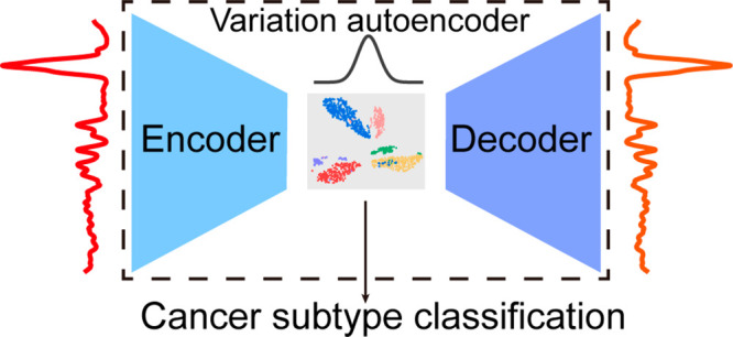
Accurate diagnosis of cancer subtypes is a great guide for the development of surgical plans and prognosis in the clinic. Raman spectroscopy, combined with the machine learning algorithm, has been demonstrated to be a powerful tool for tumor identification. However, the analysis and classification of Raman spectra for biological samples with complex compositions are still challenges. In addition, the signal-to-noise ratio of the spectra also influences the accuracy of the classification. Herein, we applied the variational autoencoder (VAE) to Raman spectra for downscaling and noise reduction simultaneously. We validated the performance of the VAE algorithm at the cellular and tissue levels. VAE successfully downscaled high-dimensional Raman spectral data to two-dimensional (2D) data for three subtypes of non-small cell lung cancer cells and two subtypes of kidney cancer tissues. Gaussian naïve bayes was applied to subtype discrimination with the 2D data after VAE encoding at both the cellular and tissue levels, significantly outperforming the discrimination results using original spectra. Therefore, the analysis of Raman spectroscopy based on VAE and machine learning has great potential for rapid diagnosis of tumor subtypes.
Introduction
Early diagnosis of cancer is highly important for improving the 10 year survival of patients. As the treatments of different subtypes have significant differences, identification of cancer subtypes is an essential reference for developing a therapy plan.1 At present, the most mainstream clinical methods are the pathological diagnosis and immunochemistry.2,3 However, these processes are too complicated and time-consuming, and the probability of misjudgment strongly relies on personal experience. Therefore, it is beneficial to develop a rapid, noninvasive, and highly sensitive technique that can accurately detect and recognize different subtypes of tumors. Raman spectroscopy is a label-free molecular vibrational spectroscopic method that can provide specific fingerprint information about the chemical composition of the biological sample, which is beneficial for clinical diagnosis.4−6 The Raman spectra consist of spectral information from nucleic acids, proteins, lipids, carbohydrates, and so on. Different types of cancer cells have different structures and compositions, corresponding to different spectra, which may lead to the possible differentiation of tumor subtypes.7−9
Raman spectra of biological samples consist of molecular information with complex composition, which makes it almost impossible to achieve the peak intensity of the target molecule directly. Therefore, an efficient analytical technique is needed to process the Raman signal. As a significant branch of machine learning, classification algorithms such as linear discriminant analysis (LDA) and supporting vector machine (SVM) are currently the most common methods for analyzing Raman spectra.6,10−14 These classification algorithms commonly distinguish Raman spectra by mining the differences between data belonging to different classes. Instead of the traditional method of extracting peak intensity, these algorithms process the entire information on the spectra when classifying them, and the more comprehensive information makes it more accurate.15,16 Currently, researchers have implemented algorithms to discriminate Raman spectra of tumors at the cellular and tissue levels.17−19
Although Raman spectroscopy has been shown to be applicable for the identification of cancer subtypes, there is still a problem that may affect the application of the classifier: feature redundancy.20−23 The spectra consist of hundreds or even thousands of data points, which make up multiple Raman peaks in the spectrum. But not every Raman peak contributes to distinguish different types of Raman spectra. Thus, unimportant data points may create feature redundancy that can have a negative impact on the classification performance. At present, the feature selection method based on variance thresholding is a common one to eliminate invalid information in machine learning, but it fails to consider the entire spectral information comprehensively and thus has limited improvement on the spectra classification.24−26 In addition, a poor signal-to-noise ratio means that the intensity of the weaker peaks is highly susceptible to being masked or affected by noise, thus affecting the classification effect. These deficiencies make the classification algorithms ineffective in differentiating Raman spectra of different tumor subtypes, which consist of similar compositions.
In this work, we combined the nine classification algorithms with Raman spectroscopy to distinguish the subtypes of cancers. The variational autoencoder (VAE) was employed to reduce feature redundancy and to accomplish noise reduction. Some studies have been conducted using autoencoders (e.g., sparse autoencoder) to process spectra for improved analysis in fields such as tumor types, microplastics, and drug resistance.27−29 However, the application of autoencoders for classifying tumor subtypes is still lacking. VAE encodes Raman spectra as two-dimensional (2D) information, which fits a Gaussian distribution, and the fewer data dimensions make it insufficient to store noise information.30−32 Nine classification models were trained to classify the VAE-encoded Raman spectra of three subtypes of non-small cell lung cancer (NSCLC) cell lines (A549, H1299, and H460) and two subtypes of kidney cancer tissues (clear cell renal cell carcinomas (CCRCC) and papillary renal cell carcinoma (PRCC)). Meanwhile, we compared the classification performance of different classifiers for both the original spectra and the VAE-compressed data, and the results show that the VAE-processed data generally give better classification results. For NSCLC cells, the Gaussian naïve bayes (NB) achieves the best classification result with an accuracy of 89.6%. For kidney cancer data, the Gaussian NB represented the best classification performance with an accuracy of 81.4%.
Materials and Methods
Cell Culture and Preparation
The three different types of human non-small cell lung cancer (NSCLC) cell lines A549, H1299, and H460 were obtained from American Type Culture Collection (ATCC). All cells were cultured in DMEM with 10% fetal bovine serum, 100 U·mL–1 penicillin, and 100 μg·mL–1 streptomycin at 37 °C in a cell incubator with 5% CO2. The mentioned reagents were bought from Gibco. Before the Raman measurements were performed, the NSCLC cell lines were washed with phosphate-buffered solution (PBS) and fixed with 4% paraformaldehyde for 10 min at room temperature. Then the cells were purified with ultrapure water to remove paraformaldehyde.
Clinical Sample Acquisition and Pathological Diagnosis
All kidney cancer tissues were acquired from patients who were diagnosed with kidney cancer with a preoperative imaging technique. The tissues were excised intraoperatively or removed by biopsy. A total of 30 patient samples were retrieved, including 16 CCRCC and 14 PRCC. The diameter of each tissue was about 1–2 mm. The acquisition of tissue samples and all experiments in this study were approved by the Ethics Committee of Renji Hospital, School of Medicine, Shanghai Jiao Tong University. The pathological diagnoses, as the gold standard for classification results, were accomplished with the standard procedure in Renji Hospital of Shanghai Jiao Tong University. All tissues were stored in a 0 °C environment until Raman spectra were collected.
Raman Spectra Acquisition
Raman spectra were obtained on a confocal Raman system (Horiba, XploRA PLUS) from the fixed cells on quartz plates. For the acquisition of cell Raman spectra, a laser beam of 532 nm was used as an excitation source. The laser power was 39.1 mW on the sample with a 60×/NA 0.7 objective. Raman spectra from all cell samples were recorded in the spectral range of 400–4000 cm–1. The collection time was 2 s for each Raman spectrum. All cells were scanned with a multipoint grid containing the whole cell in steps of 0.5–2 μm. For each cell, more than 150 spectra were collected in the acquisition. After the cell spectra were measured, the nucleus was stained. The staining reagent was DNA-binding fluorescent dye 4′,6-diamidino-2-phenylindole (DAPI). Fluorescence images were acquired using a fluorescence microscope (Leica, DM 2500) to distinguish the nucleus. The spectra acquired at the acquisition location within the DAPI-stained region are considered nuclear spectra. A total of 140 NSCLC cells were collected (H1299: 58 cells; H460: 50 cells; A549: 32 cells). To balance the sample size of the subtypes in the train set, different numbers of spectra were chosen for different subtypes of cells during the training process (20 spectra for each cell nucleus and cytoplasm of H1299, 25 spectra for H460, and 35 spectra for A549). Before the Raman spectrum acquisition of kidney cancer tissues, all tissues were taken out from a 0 °C environment and placed at room temperature (26 °C) for 30 min to avoid the influence of temperature on the Raman tests.33−35 The tissues were placed on quartz plates, and the laser was illuminated through the quartz plate onto the tissues. Raman spectra from kidney cancer tissues were excited by a 785 nm laser and recorded in the spectral range of 200–1800 cm–1, and the collection time was 5 s with the laser power of 29.8 mW. The laser spot area is approximately 3 μm. For each point, two Raman spectra were acquired and took their average as the final spectrum to reduce the random noise. For each tissue, 100 spectra were collected and 30 spectra were randomly chosen to establish the data set in the case of information saturation.
Data Preprocessing
Spectral data from our experiments were preprocessed and analyzed using Python. Before analysis, the preprocessing of Raman spectral data is crucial. A strong background always exists in Raman spectra of biological samples, and noise from different sources also contributes to the Raman signal. Removing the background and other noise before analysis is highly important. First, cell spectra were selected from all spectra according to the Raman peak between 2800 and 3000 cm–1. Then the spectra were background-subtracted. In the next step, the spectra were smoothed by employing Savitzky–Golay (SG), a filter using a polynomial order of 3 and a frame length of 15.36,37 It is a filter based on local polynomial least-squares fitting in the time domain. Afterward, we used adaptive iterative reweighted penalized least-squares (air-PLS), which iterates the least-square method to remove the baseline.38,39 The background-subtracted spectra were finally normalized to the standard normal distribution. The same process was repeated for all three types of cells. For clinical samples, the SG filter and airPLS with the same parameters as cell samples were applied to preprocess the Raman spectra.
Variational Autoencoder
The VAE consists of an encoder and a decoder. The encoder compresses the original data into a latent space (often of lower dimension than the original space), and the decoder decompresses the data in the latent space and makes it as close as possible to the original data. Unlike traditional autoencoders, for each sample, the encoder of VAE outputs not a definite value but a probability distribution, which is represented by the mean and variance of a normal distribution to ensure the continuity of the encoding. The VAE algorithm has two major advantages in the analysis of Raman spectra. The first advantage is to perform clustering of spectra. Since each spectrum is encoded as a distribution that overlaps with each other, if the distributions are from not similar spectra, then a larger loss term will be generated during training VAE. This characteristic allows classification models to be better trained and predicted from data in the latent space. The second advantage is denoising. The dimensionality of the latent space is not sufficient to support its storage of random and complex noise. Thus, VAE allows the noise to be further removed to purify the spectral information.
Before training the VAE models, data from unimportant silent regions were removed from all spectra, and each spectrum is guaranteed to have 1056 dimensions for convolution operations. Normally, a larger volume of data is desired to prevent overfitting as the number of parameters to be learned in an unsupervised learning model increases.40 A simplified VAE network architecture was designed to avoid overfitting owing to the limitation of the volume of spectral sets. The encoder was composed of four convolution layers with 1, 16, 32, and 32 kernels. All of the convolution layers have the kernel size of 4 pixels and the stride of 2. Each convolution layer is batch-normalized and followed with a 40% dropout layer to avoid overfitting. The output of the encoder was flattened and transformed by three fully connected layers with 128, 32, and 16 neurons. All of these seven layers in the encoder employed ReLU as activation functions. Finally, a fully connected layer with two neurons was used to map the output to the latent space. The decoder has the opposite network architecture to the encoder, except that the last convolutional layer, which has only one filter, does not have any activation function to output the predicted spectra. The loss function of VAE was defined as Kullback–Leibler (KL) divergence +0.9* root-mean-square errors between input spectra and predicted spectra.41−43 The batch size of VAE training was 50.
All VAE models were accomplished with Keras in Python and used the stochastic gradient descent optimizer with a learning rate of 0.0005 and momentum of 0.9.
Classification Using Machine Learning
All Raman spectra were split into train and test sets in a 7:3 ratio at the cell or patient level. For the classification of cells, the train set contains 98 cells (H1299: 40; H460: 35; A549: 23), and the test set contains 42 cells (H1299: 18; H460: 15; A549: 9). For kidney cancer, the train set contains 21 patients (CCRCC: 11, PRCC: 10), and the test set contains 9 patients (CCRCC: 5, PRCC: 4). Different classification models built were employed to classify original spectra after preprocessing and data in latent space separately, including random forest (RF), multilayer perception (MLP), SVM with linear kernel and radial basic function (RBF) kernel, logistic regression (LR), k nearest neighbor (KNN), Gaussian naïve bayes (NB), Adaboost, and LDA.44−51 All of the models were built with leave-one-patient-out cross-validation (LOPOCV).52,53 The LOPOCV used the Raman spectra of one patient or cell as a validation set and the others as the train set. The validation set is then looped until each patient’s data are used as the validation set for training the model. In contrast to the function of the test set, LOPOCV divides the data in the train set to validate the model for tuning parameters during the train stage.
Multiple classifiers were usually established for multiple classifications, and each classifier corresponds to a false positive rate (FPR) and a true positive rate (TPR). Here, FPR and TPR are defined with the following formulas:
where FP, TN, FN, and TP are the number of false positive, true negative, false negative, and true positive samples, respectively. Obviously, TPR and FPR will be influenced by the change of threshold which is used to determine the classes. For a classifier, we can get a TPR and FPR point pair based on its performance in the test sample. Therefore, the classifier can be mapped to a point on this plane. With adjusting the threshold used in this classifier, we can get a curve that goes through the points (0,0) and (1,1), which is the receiver operating characteristic (ROC) curve of this classifier. An overall standard is needed to evaluate the performance of multiclassifiers. Here, macroaveraging and microaveraging are employed to evaluate the general performance of machine learning models. Macro-average is the direct calculation of the FPR and TPR of each binary classifier, and their average is the area under the ROC curve (AUC) of multiclassifiers.54 The microaverage calculates the arithmetic average of TP, FP, TN, and FN of each binary classifier and then obtains the FPR and TPR of multiclassifiers according to these average values, and finally, the ROC curve and AUC are determined.
Results and Discussion
Data Set of NSCLC Cells
Lung cancer, being the second largest number of new cases, poses a serious threat to human life.55 NSCLC is the most common type of lung cancer, accounting for about 85% of lung cancers.56 We employed three different cell subtypes of NSCLC to verify the performance of Raman spectroscopy at the cellular level for subtype diagnosis. Before collecting Raman spectra, all the cell samples were fixed with 4% paraformaldehyde for 10 min. Some studies have suggested that paraformaldehyde fixation is a sample preparation method with minimal impact on biochemical information over living conditions.57,58 To the best of our knowledge, 4% paraformaldehyde fixation for 10 min is optimal for Raman studies.59,60 The remaining molecular information (such as proteins and lipids) on cell samples is sufficient to distinguish between cell types.61,62 The whole-cell Raman mapping was performed on each cell model in this work, and the cell nuclei were stained with DAPI to distinguish the nucleus boundary in the cell after Raman acquisition. From the example Raman spectrum in the range of 200–4000 cm–1 (Figure S1a), the background signal almost obscures the Raman signal in the range of 200–400 cm–1, thus the scanning ranges of all the cell samples were set to 400–4000 cm–1. For each cell, more than 150 Raman spectra were measured in acquisition with a 532 nm laser. Compared to the common 785 nm laser, the 532 nm laser could acquire the more significant Raman signals of the C–H bond for the cellular spectra, although it excites a stronger fluorescence signal. The fluorescence background can be removed by baseline correction. Figure 1 shows the bright-field images, Raman mapping images (plotted by the Raman bands between 2700 and 3100 cm–1), DAPI-stained fluorescent images, and the average normalized Raman spectra of three subtypes of NSCLC of A549, H1299, and H460. The cancer cells have large heterogeneity so that the size and morphology are not reliable evidence for identifying the subtypes of NSCLC cells. An obvious Raman band can be detected in the spectral region between 2700 and 3100 cm–1 (Figure 1iv), which is the stretching vibration mode of the C–H bond. This band originates from two main aliphatic C–H bonds located at 2854 and 2940 cm–1 and other abundant C–H bonds belonging to various biomolecules. Hobro et al. showed that, although the use of paraformaldehyde fixation has an influence on this region, its influence is very weak relative to the Raman intensity of this region.57Figure S2 shows the Raman spectra at different detection positions (point 1, quartz; point 2, cytoplasm; point 3, nucleus), indicating that no significant Raman bands exist in this spectral range on the quartz substrate. Therefore, the intensity of the Raman signal between 2700 and 3100 cm–1 can be utilized to determine whether the spectrum is inside the cell (shown in Figure 1ii). The clearer cell boundaries are shown in Figure S2 by overexposed heatmaps. The area of the nucleus is characterized by DAPI staining, and therefore, we can further separate the Raman spectra from the nucleus and cytoplasm (Figure 1iii). It can be found that there are slight differences in the Raman spectra between the nucleus and cytoplasm for different cells (Figure S2). The Raman signal from 2100 to 2700 cm–1 was removed from the spectra as this range is in the biological transparency window, and typically, it does not affect subsequent data analysis.63,64
Figure 1.

(i) Bright-field images, (ii) Raman mapping images plotted by the shaded Raman band between 2700 and 3100 cm–1, (iii) DAPI-stained fluorescent images, (iv) their overlay images, and (v) mean Raman spectra from (a) A549, (b) H460, and (c) H1299 NSCLC cell lines. The scale bars in panel (i) are 10 μm. The blue curves represent the mean Raman spectra only from the nuclei region, and red curves represent spectra only from the cytoplasm region. The shaded areas along the spectra represent the standard deviations of the means.
Classification of Different Cellular Raman Data Sets
To compare the effects of data from different parts of a cell on the classification effect, we established four different SVM with RBF kernel models based on different data sets: (1) nuclear model, where the data set consists of spectra of cell nucleus only; (2) cytoplasmic model, where the data set consists of spectra of cell cytoplasm only; (3) cell model, where the data set consists of all spectra of three subtypes of NSCLC cells; the model only outputs the cell subtype no matter if the spectrum is from the nucleus or cytoplasm; (4) six-classes model, where the data set consists of spectral data of the nucleus and cytoplasm of three subtypes of cells. Therefore, it contains six classes of spectral data. The model outputs the cell subtype to which the spectrum belongs along with whether it is a cytoplasmic or nuclear spectrum. SVM is the classical algorithm used for classification based on Raman spectra. The train set consists of the spectra from 98 cells (40 cells for H1299, 35 cells for H460, and 23 cells for A549). To balance the sample size of each cell subtype in the train set, 20 spectra were randomly selected for each cell nucleus and cytoplasm of H1299, 25 spectra for H460, and 35 spectra for A549. Each spectrum was standardized after smoothing and baseline correction. The LOPOCV method was used to evaluate the classification performance of the model on the train set. To assess the classification performance of the machine learning models on unknown data, we adopt the Raman spectra from 42 other cells (18 cells for H1299, 15 cells for H460, and 9 cells for A549) as the test set.
For the SVM classifier with more than two classes, the model outputs the classification scores which represent the relative probabilities that every spectrum belongs to every class and takes the class with the maximum probability as the final classification result. Figure 2i shows the classification scores of every spectrum in the test set, which are predicted by the SVM models based on the entire spectral information. For the six-classes model, we visualize the 6D classification scores on 3D space using t-distributed stochastic neighbor embedding (t-SNE). t-SNE is a powerful technology to visualize high-dimensional data in low-dimensional space while preserving the original distribution of the data. As can be seen from the collection of data points of different colors and shapes, spectra belonging to different types were successfully separated. The results show that the SVM has good classification performance for all four models. Even for the complex six-classes model which distinguishes the cytoplasm and nucleus of different cell types, different types of data points can still be separated.
Figure 2.

(i) Graphic classification results and (ii) ROC curves and AUC values of four SVM models based on different types of data sets: (a) cytoplasmic model, (b) nuclear model, (c) cell model, (d) six-classes model. The gray dashed lines represent the ROC curves for the completely random guesses.
The classification model mostly provides the relative probability that the spectrum is positive. If the classification score is greater than the specified threshold, it will be distinguished as a positive sample; otherwise, it is a negative sample. As thresholds change, common performance indicators will be influenced, such as FPR and TPR. Therefore, we introduce the ROC curve to measure the performance of the model at full thresholds. As shown in Figure 2ii, we depicted the ROC curves of every model. The micro- and macroaverage ROC curves also were calculated with the ROC curves of every single classifier to evaluate the general performance of the classification model (see the details in Materials and Methods). Meanwhile, the AUC values were calculated to evaluate the model performance numerically. For every model, the AUC value of the classifier with H460 as the positive sample is significantly superior to the other classifiers. This result indicates that the classification performance of the model to H460 is better. All AUC values are higher than 0.8, which means that the classification performances of the four models are credible. The classification results are shown in Table 1. The results at the spectrum level refer to the percentage of all spectra that are accurately classified. The accuracies on the cell level are developing statistics of the result at the spectral level that select the class with the highest number of classification spectra in a cell as the final predicted class of this cell. Although the accuracy of the six-classes model is slightly lower than that of the other three models at the spectral level, it achieves 100% accuracy at the cellular level. Therefore, the six-classes model is considered to obtain the best classification results for cells.
Table 1. SVM Result of the Distinction between Three Subtypes of NSCLC.
| model | level | LOPOCV (%) | accuracy (%) |
|---|---|---|---|
| nuclear model | spectrum | 92.5 | 91.9 |
| cell | 97.6 | ||
| cytoplasmic model | spectrum | 90.1 | 88.4 |
| cell | 97.6 | ||
| cell model | spectrum | 90.5 | 89.2 |
| cell | 97.6 | ||
| six-classes model | spectrum | 85.7 | 83.3 |
| cell | 100 |
VAE Dimensionality Reduction of Cellular Data
In the fingerprint and C–H regions, there is rich information on biomolecular Raman bands, giving them the potential to distinguish different subtypes of cells. However, the abundant molecular species may cause feature redundancy, which means some bands are indistinguishable between different subtypes of cancer cells. Meanwhile, noise is another main factor affecting classification performance. The VAE was employed to mitigate the effects of feature redundancy and noise. Figure 3 shows the schematic representation of VAE. The VAE consists of an encoder, which compresses the Raman spectral data into a 2D latent space, and a decoder, decoding the 2D data from the latent space into a spectrum. The encoder compresses the Raman spectrum into data points that fit a Gaussian distribution. The latent space formed by the neurons at the end of the encoder is often only two or three dimensions, which makes it insufficient to store randomly occurring noise signals, thus simultaneously achieving noise reduction and dimensionality reduction. The VAE uses a convolutional network architecture, and the specific architecture and training details are described in Materials and Methods.
Figure 3.
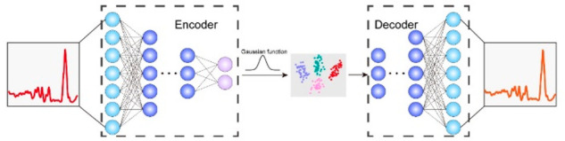
Schematic representation of the principle of VAE. VAE consists of two parts including an encoder and a decoder. The encoder downscales the input Raman spectra into a 2D latent space. In the latent space, similar data points will be relatively closer. The decoder converts the downscaled 2D data points back to Raman spectra.
As shown in Figure 4a, the data points of different classes, which are represented by different shapes and colors, are trained to fit the Gaussian distribution in the latent space. The spectra with similarities are grouped into the same cluster, while those that are not similar are separated. Figure 4b visualizes the train loss and test loss of the VAE with the increase of epochs. The loss represents the KL divergence and the root-mean-square errors between the input spectra and predicted spectra (see the details in Materials and Methods). Rapid reduction of both the train loss and test loss after 30 epochs represents that the fast convergence of the VAE model, which suggests strong reliability of the VAE for prediction. Figure 4c exhibits the comparisons between the VAE-generated spectra of the central points of every cluster in the latent space and the mean spectra from the same class of NSCLC spectra. The great similarity between the practical spectra and the VAE-generated spectra indicates that the clustering behavior of the VAE encoder reflects the similarity trend of the practical spectral distribution. In addition, the spectra generated by VAE have the characteristics of low noise like the average spectrum, indicating that VAE contributes to noise reduction. Meanwhile, the stochastic original spectra and the corresponding VAE-generated spectra shown in Figure S3 indicate that the VAE can perform noise filtering while preserving the spectral features in the process of encoding and compression.
Figure 4.

Graphic representation of the VAE on the test set for different subtypes of NSCLC cells. (a) VAE-encoded space of NSCLC spectra. (b) Loss function of VAE on the training set and test set. (c) Experiment-acquired averaged Raman spectra (red) and VAE-generated spectra (blue) from the centers of different classes: (i) A549 cytoplasm; (ii) A549 nuclei; (iii) H460 cytoplasm; (iv) H460 nuclei; (v) H1299 cytoplasm; (vi) H1299 nuclei. (d) ROC curves of Gaussian NB and SVM with RBF kernel models based on VAE-encoded data and original spectra of subtypes of NSCLC. The gray dashed lines represent the ROC curves for the completely random guesses.
The redundant features are confirmed to be removed by calculating both correlations between features and variances of features. The variances for every feature of original spectral data and VAE-encoded data in the train set were calculated to detect the significance of the features. Features with low variance usually include useless information. From Figure S4a, the variances of the spectral data are all significantly smaller than VAE-encoded data, and there are variances of numerous features close to 0. This result indicates that the useless features are removed by the dimension reduction of VAE. The Pearson correlation coefficient (PCC) was applied to compute the correlation between features. The absolute value of PCC is in the range of 0 to 1, and the closer to 1 shows the higher correlation. A strong correlation between features represents the duplication of the information contained in the features. Usually, an absolute value of PCC greater than 0.5 represents a relatively strong correlation.65 The statistical results of PCC values suggest a relatively strong correlation between numerous features of the original spectral data (Figure S4b). In contrast, the correlation between the two features after VAE encoding is extremely weak (the absolute PCC is 0.036), which indicates the features are independent of each other. These results prove that the redundant features are effectively removed after dimension reduction by VAE.
Classification of VAE-Encoded Cellular Data
To verify the improvement of the classification performance by VAE, we trained the nine machine learning algorithms based on the same training set to classify the spectra of different subtypes of NSCLC cells through the entire spectral information and the data in latent space, including RF, MLP, SVM with linear kernel, SVM with RBF kernel, LR, KNN, Gaussian NB, Adaboost, and LDA. Because of the better classification performance at the cellular level, the six-classes model was used to evaluate the classification performance of every algorithm. For every classification model trained by entire spectral information, the feature selection method based on variance thresholding is used to remove low variance features. We only included 200 features before model training to prevent overfitting.
As shown in Table 2, for each algorithm, the accuracy of the classifier trained using the VAE-encoded data was generally higher than that of the classifier trained using the entire spectral information. The accuracy improvement varies among different classification algorithms, indicating that there are discrepancies in the improvement effect of VAE on different algorithms. Raman spectra are high-dimensional data and have high correlations between adjacent features because the peaks possess a certain width. After dimension reduction by VAE, the dimension of data turns into two dimensions, and the features are relatively independent from each other. Therefore, for algorithms that are appropriate for low-dimensional or low-relevance data, their classification accuracies will be significantly improved after dimension reduction by VAE, such as Adaboost and Gaussian NB.66 In contrast, for algorithms suitable for high-dimensional data, the improvements in classification accuracies after dimension reduction are not significant, such as MLP.67 Among them, Gaussian NB achieved the best classification results for the VAE-encoded data, and SVM with the RBF kernel had the best results for the entire spectral information. A similar result can also be proven by the ROC curves of these two classification models in Figure 4d. SVM with the RBF kernel has a great advantage for the classification of nonlinear high-dimensional data. In contrast, Gaussian NB has better classification performance for low-dimensional data. The role of VAE is to compress high-dimensional data into low-dimensional data. Therefore, Gaussian NB produces better classification results for VAE-encoded data. As shown in Figure 4d, the ROC curves of the Gaussian NB and SVM with RBF kernel models trained with the entire spectral information are relatively weaker, indicating that the dimensionality reduction process of VAE has a beneficial performance on the classification models.
Table 2. Classification Result of Nine Models on Six Classes of NSCLC Cell Spectra with and without VAE.
| without VAE |
with VAE |
|||
|---|---|---|---|---|
| model | LOPOCV (%) | accuracy (%) | LOPOCV (%) | accuracy (%) |
| Gaussian NB | 81.4 | 80.7 | 89.6 | 89.6 |
| RF | 83.2 | 83.0 | 88.5 | 88.0 |
| SVM (RBF) | 85.7 | 83.3 | 88.4 | 86.3 |
| SVM (linear) | 83.7 | 83.3 | 88.3 | 88.6 |
| LDA | 84.3 | 83.6 | 87.9 | 87.7 |
| LR | 82.9 | 81.6 | 86.3 | 85.7 |
| Ada | 78.7 | 75.3 | 87.7 | 86.4 |
| KNN | 77.0 | 75.2 | 84.7 | 83.7 |
| MLP | 80.2 | 79.7 | 81.3 | 81.1 |
We also established four Gaussian NB models based on different data sets (nuclear model, cytoplasmic model, cell model, and six-classes model). The accuracies and ROC curves of these four Gaussian NB models on the test set are shown in Table S1 and Figure S5. It can be found that all four Gaussian NB models show superior performance to the SVM models (see Table 1), and the accuracy can reach 100% on the cell level for each model.
We also compared the influence of four dimension reduction methods on the classification performance including principal component analysis (PCA), t-SNE, uniform manifold approximation and projection (UMAP), and VAE (Table S2). The LDA, Gaussian NB, and SVM algorithms that perform effectively on low-dimensional data were selected for the classification of data after dimensionality reduction. The LOPOCVs and accuracies of the algorithms were computed to evaluate the classification performances (Table S2). The results showed that UMAP and VAE were significantly superior to PCA and t-SNE in improving the classification results. Although the improvement of LDA classification by UMAP is better than VAE, the combination of VAE and Gaussian NB still achieves the best classification performance. Therefore, compared with other three dimension reduction algorithms, VAE can effectively perform dimension reduction and improve the classification performance.
VAE Dimensionality Reduction of Kidney Cancer Data
To further validate the performance of Raman spectroscopy combined with VAE for cancer diagnosis on the tissue level, we collected Raman spectra of kidney cancer tissues from patients removed by surgery or puncture and established the machine learning models for in vitro cancer subtype diagnosis. Kidney cancer caused about 180,000 deaths, and the incidence is gradually increasing at a rate of 2.2% in 2020.55 We retrieved tumor tissues from 16 CCRCC patients and 14 PRCC patients for evaluation. The scanning ranges were set to 200–1800 cm–1 for all tissue samples due to the weak Raman signal after the biological transparency window (Figure S1b). For each tissue, approximately 100 Raman spectra were acquired, but in the case of signal saturation, some of the spectra were excluded and typically only 30 spectra of the tumor tissue were employed to train and test the machine learning models after preprocessing. We calculated the PCC between the average spectra of 100 spectra and 30 spectra. The PCC shows that there is a strong correlation between the two mean spectra (PCCs > 0.95), which means that the tissue information derived from 30 spectra is almost equivalent to 100 spectra. Raman spectra of 70% of the patient samples (11 CCRCC and 10 PRCC) were used as the train set to train the VAE model and the classification models, and the remaining spectra were used to perform model performance tests.
Figure 5 shows the results achieved by the trained VAE model on the test set. As shown in Figure 5a, a commendable differentiation effect can be achieved for the data set of the two subtypes of kidney cancer in the latent space of VAE. Data points of the same subtype are clustered together, while data points of different subtypes are aggregated into different clusters. VAE maintains the original similarity relationship of the data well while performing dimensionality reduction of Raman spectra of kidney cancer. The convergences, consisting of the KL divergences and mean square errors between the decoded spectra and practical spectra in train and test processes, are shown in Figure 5b. Both the train loss and the test loss converge after 50 epochs, demonstrating that the VAE model is robust to the encoding and decoding process of kidney cancer data. Figure 5c demonstrates the comparisons between the VAE-generated spectra of the central points of different clusters in the latent space and the mean spectra of different subtypes of cancer. Similar to the cell results, the agreement between the mean spectra and generated spectra suggests that the VAE accomplishes both spectral information compression and noise reduction. The variances and correlation coefficients indicate that the useless and highly correlated features were removed after the dimension reduction of VAE (Figure S6).
Figure 5.

Graphic representation of the VAE on the test set for two subtypes of kidney cancer. (a) VAE-encoded space of kidney cancer spectra. (b) Loss function of VAE on the training set and test set. (c) Experiment-acquired averaged Raman spectra (red) and VAE-generated spectra from the centers of different subtypes, (i) CCRCC and (ii) PRCC, of kidney cancer spectra (blue). Insets in panel (c) show pathological images of two subtypes. The scale bars are 1 mm. (d) Graphic classification results of RF based on the original spectra. (e) ROC curves of Gaussian NB and RF based on VAE-encoded data and original spectra of subtypes of kidney cancer.
Classification of Kidney Cancer
The same nine algorithms were trained based on the validation of LOPOCV to classify different subtypes of kidney cancer tissues through entire spectral information and VAE-encoded data in latent space, respectively. Table 3 represents the classification results of nine models on VAE-encoded spectral data of kidney cancer. It shows that Gaussian NB achieves the best performance among the nine classification algorithms, with a differentiation accuracy of 81.4% and an AUC value of 0.835. In addition, the classification of the data using VAE after dimensionality reduction is generally better compared with the results obtained using the entire spectral information (Table S3). Figure 5d shows the classification effect of the RF, which achieves the best performance based on the entire spectral information on the test set. The two axes represent the probability that the spectral data belong to the two subtypes calculated by RF. The results demonstrated that the split between the data of the two subtypes was not apparent. We also compared the ROC curves of RF and Gaussian NB based on both the entire spectral information and VAE-encoded data (Figure 5e). The ROC curves of the Gaussian NB classifier based on the VAE-encoded data are significantly better than those of the other three classifiers, indicating that VAE could significantly improve classification performance with the help of Gaussian NB. Thus, it demonstrates that VAE performs effective information purification and noise reduction for the spectra of kidney cancer. At the same time, the accuracy of up to 81.4% proves that Raman spectroscopy combined with VAE is an effective tool for in vitro biopsy of subtypes of kidney cancer, therefore aiding the surgeon in designing the surgical plan.
Table 3. Classification Results of Nine Models on VAE-Encoded Data of Kidney Cancer Spectra.
| model | LOPOCV (%) | accuracy (%) | AUC |
|---|---|---|---|
| Gaussian NB | 82.7 | 81.4 | 0.835 |
| LDA | 80.6 | 80.2 | 0.823 |
| LR | 79.3 | 78.9 | 0.795 |
| MLP | 79.2 | 78.4 | 0.806 |
| SVM (RBF) | 79.2 | 78.7 | 0.793 |
| KNN | 79.1 | 77.6 | 0.785 |
| SVM (linear) | 78.5 | 76.4 | 0.777 |
| RF | 78.5 | 77.3 | 0.783 |
| Ada | 73.4 | 72.6 | 0.747 |
Conclusions
In summary, we developed an analysis technique based on the label-free Raman spectroscopy to identify tumor subtypes. We applied an autoencoder network of VAE to attenuate the effects of high feature dimensionality and noise. VAE downscales Raman spectral data in high-dimensional space to a low-dimensional space (only two dimensions) and maintains the Gaussian distribution in the latter. The low-dimensional information in the latent space of VAE makes it impossible to store randomly occurring noise information for noise reduction purposes. Among nine types of machine learning algorithms combined with VAE, Gaussian NB achieved the best performance to classify the cell data from three subtypes of NSCLC and the tissue data from two subtypes of kidney cancer. In contrast to the conventional SVM algorithms, Gaussian NB improves the classification accuracy from 83.3 to 89.6% at the cellular level and from 77.5 to 81.4% at the tissue level. These results suggest that the analysis of Raman spectra using the VAE-combined machine learning algorithms can assist physicians in making rapid, noninvasive, and more accurate discrimination of the subtypes of cancer cells and tissues. It is of great significance for both the development of surgical plans and postoperative drug administration.
Acknowledgments
We gratefully acknowledge the financial support from the National Natural Science Foundation of China (No. 81871401), the Science and Technology Commission of Shanghai Municipality (Nos. 19441905300 and 21511102100), Shanghai Jiao Tong University (No. YG2019QNA28), and the Shanghai Key Laboratory of Gynecologic Oncology.
Supporting Information Available
The Supporting Information is available free of charge at https://pubs.acs.org/doi/10.1021/acsomega.1c07263.
Additional examples of Raman spectra, materials, and results, including supplemental tables for Gaussian NB performance of different cell subtypes and kidney cancer (PDF)
Author Contributions
J.Y. and C.H. conceived the idea. S.Z. performed the cell experiment and collected Raman spectra of cells. Y.C. and X.W. performed the surgeries and obtained tissue samples. J.Z. preprocessed and stored tissues before Raman acquisition. C.H. collected and analyzed Raman spectra of cells and tissues. J.Y. administrated the project and provided the guidance of methodology. All authors contributed the writing and revising of the manuscript.
The authors declare no competing financial interest.
Supplementary Material
References
- Wild C.; Weiderpass E.; Stewart B. W.. World Cancer Report: Cancer Research for Cancer Prevention; IARC Press, 2020. [Google Scholar]
- Rorke L. B. Pathologic diagnosis as the gold standard. Cancer 1997, 79 (4), 665–667. 10.1002/(SICI)1097-0142(19970215)79:4<665::AID-CNCR1>3.0.CO;2-D. [DOI] [PubMed] [Google Scholar]
- Compérat E.; Varinot J. Immunochemical and molecular assessment of urothelial neoplasms and aspects of the 2016 World Health Organization classification. Histopathology 2016, 69 (5), 717–726. 10.1111/his.13025. [DOI] [PubMed] [Google Scholar]
- Long D. A.Raman Spectroscopy; McGraw-Hill: New York, 1977; pp 1–12. [Google Scholar]
- Mulvaney S. P.; Keating C. D. Raman spectroscopy. Anal. Chem. 2000, 72 (12), 145–158. 10.1021/a10000155. [DOI] [PubMed] [Google Scholar]
- Siraj N.; Bwambok D. K.; Brady P. N.; Taylor M.; Baker G. A.; Bashiru M.; Macchi S.; Jalihal A.; Denmark I.; Le T.; Elzey B.; Pollard D. A.; Fakayode S. O. Raman spectroscopy and multivariate regression analysis in biomedical research, medical diagnosis, and clinical analysis. Appl. Spectrosc. Rev. 2021, 56, 615–672. 10.1080/05704928.2021.1913744. [DOI] [Google Scholar]
- Fan Y.; Duan X.; Zhao M.; Wei X.; Wu J.; Chen W.; Liu P.; Cheng W.; Cheng Q.; Ding S. High-sensitive and multiplex biosensing assay of NSCLC-derived exosomes via different recognition sites based on SPRi array. Biosens. Bioelectron. 2020, 154, 112066. 10.1016/j.bios.2020.112066. [DOI] [PubMed] [Google Scholar]
- O’Dea D.; Bongiovanni M.; Sykiotis G. P.; Ziros P. G.; Meade A. D.; Lyng F. M.; Malkin A. Raman spectroscopy for the preoperative diagnosis of thyroid cancer and its subtypes: An in vitro proof-of-concept study. Cytopathology 2019, 30 (1), 51–60. 10.1111/cyt.12636. [DOI] [PubMed] [Google Scholar]
- Talari A. C. S.; Evans C. A.; Holen I.; Coleman R. E.; Rehman I. U. Raman spectroscopic analysis differentiates between breast cancer cell lines. JRSp 2015, 46 (5), 421–427. 10.1002/jrs.4676. [DOI] [Google Scholar]
- Ralbovsky N. M.; Lednev I. K. Towards development of a novel universal medical diagnostic method: Raman spectroscopy and machine learning. Chem. Soc. Rev. 2020, 49 (20), 7428–7453. 10.1039/D0CS01019G. [DOI] [PubMed] [Google Scholar]
- Jordan M. I.; Mitchell T. M. Machine learning: Trends, perspectives, and prospects. Science 2015, 349 (6245), 255–260. 10.1126/science.aaa8415. [DOI] [PubMed] [Google Scholar]
- Jermyn M.; Mok K.; Mercier J.; Desroches J.; Pichette J.; Saint-Arnaud K.; Bernstein L.; Guiot M.-C.; Petrecca K.; Leblond F. Intraoperative brain cancer detection with Raman spectroscopy in humans. Sci. Transl. Med. 2015, 7 (274), 274ra19. 10.1126/scitranslmed.aaa2384. [DOI] [PubMed] [Google Scholar]
- He C.; Wu X. R.; Zhou J. L.; Chen Y. H.; Ye J. Raman optical identification of renal cell carcinoma via machine learning. Spectrochim. Acta, Part A 2021, 252, 119520. 10.1016/j.saa.2021.119520. [DOI] [PubMed] [Google Scholar]
- Zhang Y. Q.; Ye X. J.; Xu G. X.; Jin X. L.; Luan M. M.; Lou J. T.; Wang L.; Huang C. J.; Ye J. Identification and distinction of non-small-cell lung cancer cells by intracellular SERS nanoprobes. RSC Adv. 2016, 6 (7), 5401–5407. 10.1039/C5RA21758J. [DOI] [Google Scholar]
- Lee D.; Seung H. S. Algorithms for non-negative matrix factorization. Adv. Neural Inf. Process. Syst. 2000, 13, 556–562. [Google Scholar]
- Shen Y.; Yue J.; Xu W.; Xu S. Recent progress of surface-enhanced Raman spectroscopy for subcellular compartment analysis. Theranostics 2021, 11 (10), 4872. 10.7150/thno.56409. [DOI] [PMC free article] [PubMed] [Google Scholar]
- Zhou Y.; Liu C. H.; Wu B.; Yu X.; Cheng G.; Zhu K.; Wang K.; Zhang C.; Zhao M.; Zong R.; Zhang L.; Shi L.; Alfano R. R. Optical biopsy identification and grading of gliomas using label-free visible resonance Raman spectroscopy. J. Biomed. Opt. 2019, 24 (9), 1–12. 10.1117/1.JBO.24.9.095001. [DOI] [PMC free article] [PubMed] [Google Scholar]
- Zhang K.; Hao C.; Huo Y.; Man B.; Zhang C.; Yang C.; Liu M.; Chen C. Label-free diagnosis of lung cancer with tissue-slice surface-enhanced Raman spectroscopy and statistical analysis. Lasers Med. Sci. 2019, 34 (9), 1849–1855. 10.1007/s10103-019-02781-w. [DOI] [PubMed] [Google Scholar]
- Ibrahim O.; Toner M.; Flint S.; Byrne H. J.; Lyng F. M. The Potential of Raman Spectroscopy in the Diagnosis of Dysplastic and Malignant Oral Lesions. Cancers (Basel) 2021, 13 (4), 619. 10.3390/cancers13040619. [DOI] [PMC free article] [PubMed] [Google Scholar]
- Li S.; Chen G.; Zhang Y.; Guo Z.; Liu Z.; Xu J.; Li X.; Lin L. Identification and characterization of colorectal cancer using Raman spectroscopy and feature selection techniques. Opt. Express 2014, 22 (21), 25895–25908. 10.1364/OE.22.025895. [DOI] [PubMed] [Google Scholar]
- McShane M. J.; Cameron B. D.; Coté G. L.; Motamedi M.; Spiegelman C. H. A novel peak-hopping stepwise feature selection method with application to Raman spectroscopy. Anal. Chim. Acta 1999, 388 (3), 251–264. 10.1016/S0003-2670(99)00080-X. [DOI] [Google Scholar]
- Teofilo R. F.; Martins J. P. A.; Ferreira M. M. Sorting variables by using informative vectors as a strategy for feature selection in multivariate regression. J. Chemom. 2009, 23 (1), 32–48. 10.1002/cem.1192. [DOI] [Google Scholar]
- Jermyn M.; Desroches J.; Aubertin K.; St-Arnaud K.; Madore W.-J.; De Montigny E.; Guiot M.-C.; Trudel D.; Wilson B. C; Petrecca K.; Leblond F. A review of Raman spectroscopy advances with an emphasis on clinical translation challenges in oncology. Phys. Med. Biol. 2016, 61 (23), R370. 10.1088/0031-9155/61/23/R370. [DOI] [PubMed] [Google Scholar]
- Donoho D.; Jin J. Higher criticism thresholding: Optimal feature selection when useful features are rare and weak. Proc. Natl. Acad. Sci. U.S.A. 2008, 105 (39), 14790–14795. 10.1073/pnas.0807471105. [DOI] [PMC free article] [PubMed] [Google Scholar]
- Gautam R.; Peoples D.; Jansen K.; O’Connor M.; Thomas G.; Vanga S.; Pence I. J.; Mahadevan-Jansen A. Feature selection and rapid characterization of bloodstains on different substrates. Appl. Spectrosc. 2020, 74 (10), 1238–1251. 10.1177/0003702820937776. [DOI] [PubMed] [Google Scholar]
- Sreejith S.; Nehemiah H. K.; Kannan A. Clinical data classification using an enhanced SMOTE and chaotic evolutionary feature selection. Comput. Biol. Med. 2020, 126, 103991. 10.1016/j.compbiomed.2020.103991. [DOI] [PubMed] [Google Scholar]
- Brandt J.; Mattsson K.; Hassellov M. Deep Learning for Reconstructing Low-Quality FTIR and Raman Spectra horizontal line A Case Study in Microplastic Analyses. Anal. Chem. 2021, 93 (49), 16360–16368. 10.1021/acs.analchem.1c02618. [DOI] [PMC free article] [PubMed] [Google Scholar]
- Ciloglu F. U.; Caliskan A.; Saridag A. M.; Kilic I. H.; Tokmakci M.; Kahraman M.; Aydin O. Drug-resistant Staphylococcus aureus bacteria detection by combining surface-enhanced Raman spectroscopy (SERS) and deep learning techniques. Sci. Rep. 2021, 11 (1), 18444. 10.1038/s41598-021-97882-4. [DOI] [PMC free article] [PubMed] [Google Scholar]
- Aslam M. A.; Xue C.; Chen Y.; Zhang A.; Liu M.; Wang K.; Cui D. Breath analysis based early gastric cancer classification from deep stacked sparse autoencoder neural network. Sci. Rep. 2021, 11 (1), 4014. 10.1038/s41598-021-83184-2. [DOI] [PMC free article] [PubMed] [Google Scholar]
- Kingma D. P.; Welling M.. Auto-encoding variational bayes. arXiv 2013; https://arxiv.org/abs/1312.6114. [Google Scholar]
- Pu Y.; Gan Z.; Henao R.; Yuan X.; Li C.; Stevens A.; Carin L.. Variational autoencoder for deep learning of images, labels and captions. arXiv 2016; https://arxiv.org/abs/1609.08976. [Google Scholar]
- Kusner M. J.; Paige B.; Hernández-Lobato J. M. Grammar variational autoencoder. ICML 2017, 1945–1954. [Google Scholar]
- Krishnan K. Influence of temperature on the Raman effect. Nature 1928, 122 (3078), 650–650. 10.1038/122650b0. [DOI] [Google Scholar]
- Bauer N. J.; Motamedi M.; Hendrikse F.; Wicksted J. P. Remote temperature monitoring in ocular tissue using confocal Raman spectroscopy. J. Biomed. Opt. 2005, 10 (3), 031109. 10.1117/1.1911901. [DOI] [PubMed] [Google Scholar]
- Ghita A.; Matousek P.; Stone N. Sensitivity of Transmission Raman Spectroscopy Signals to Temperature of Biological Tissues. Sci. Rep. 2018, 8 (1), 8379. 10.1038/s41598-018-25465-x. [DOI] [PMC free article] [PubMed] [Google Scholar]
- Barton S. J.; Ward T. E.; Hennelly B. M. Algorithm for optimal denoising of Raman spectra. Anal. Methods 2018, 10 (30), 3759–3769. 10.1039/C8AY01089G. [DOI] [Google Scholar]
- Savitzky A.; Golay M. J. Smoothing and differentiation of data by simplified least squares procedures. Anal. Chem. 1964, 36 (8), 1627–1639. 10.1021/ac60214a047. [DOI] [Google Scholar]
- Zhang Z.-M.; Chen S.; Liang Y.-Z. Baseline correction using adaptive iteratively reweighted penalized least squares. Analyst 2010, 135 (5), 1138–1146. 10.1039/b922045c. [DOI] [PubMed] [Google Scholar]
- Boelens H. F.; Dijkstra R. J.; Eilers P. H.; Fitzpatrick F.; Westerhuis J. A. New background correction method for liquid chromatography with diode array detection, infrared spectroscopic detection and Raman spectroscopic detection. J. Chromatogr. A 2004, 1057 (1–2), 21–30. 10.1016/j.chroma.2004.09.035. [DOI] [PubMed] [Google Scholar]
- Nakkiran P.; Kaplun G.; Bansal Y.; Yang T.; Barak B.; Sutskever I. Deep double descent: Where bigger models and more data hurt. J. Stat. Mech. 2021, 2021 (12), 124003. 10.1088/1742-5468/ac3a74. [DOI] [Google Scholar]
- Hershey J. R.; Olsen P. A. Approximating the Kullback Leibler divergence between Gaussian mixture models. ICASSP IEEE 2007, IV-317. 10.1109/ICASSP.2007.366913. [DOI] [Google Scholar]
- Lim K.-L.; Jiang X.; Yi C. Deep clustering with variational autoencoder. ISPL 2020, 27, 231–235. 10.1109/LSP.2020.2965328. [DOI] [Google Scholar]
- Thrift W. J.; Ronaghi S.; Samad M.; Wei H.; Nguyen D. G.; Cabuslay A. S.; Groome C. E.; Santiago P. J.; Baldi P.; Hochbaum A. I.; Ragan R. Deep Learning Analysis of Vibrational Spectra of Bacterial Lysate for Rapid Antimicrobial Susceptibility Testing. ACS Nano 2020, 14 (11), 15336–15348. 10.1021/acsnano.0c05693. [DOI] [PubMed] [Google Scholar]
- Svetnik V.; Liaw A.; Tong C.; Culberson J. C.; Sheridan R. P.; Feuston B. P. Random forest: a classification and regression tool for compound classification and QSAR modeling. J. Chem. Inf. Comput. Sci. 2003, 43 (6), 1947–1958. 10.1021/ci034160g. [DOI] [PubMed] [Google Scholar]
- Jain A.K.; Jianchang Mao; Mohiuddin K.M. Artificial neural networks: A tutorial. Comp 1996, 29 (3), 31–44. 10.1109/2.485891. [DOI] [Google Scholar]
- Huang S. J.; Cai N. G.; Pacheco P. P.; Narandes S.; Wang Y.; Xu W. N. Applications of Support Vector Machine (SVM) Learning in Cancer Genomics. Cancer Genom. Proteom. 2018, 15 (1), 41–51. [DOI] [PMC free article] [PubMed] [Google Scholar]
- Pregibon D. Logistic regression diagnostics. Ann. Stat. 1981, 9 (4), 705–724. 10.1214/aos/1176345513. [DOI] [Google Scholar]
- Peterson L. E. K-nearest neighbor. Scholarpedia 2009, 4 (2), 1883. 10.4249/scholarpedia.1883. [DOI] [Google Scholar]
- Murphy K. P.Naive bayes classifiers. University of British Columbia, 2006, Vol. 18 (60).
- Hastie T.; Rosset S.; Zhu J.; Zou H. Multi-class adaboost. Stat. Interface 2009, 2 (3), 349–360. 10.4310/SII.2009.v2.n3.a8. [DOI] [Google Scholar]
- Tharwat A.; Gaber T.; Ibrahim A.; Hassanien A. E. Linear discriminant analysis: A detailed tutorial. AI Commun. 2017, 30 (2), 169–190. 10.3233/AIC-170729. [DOI] [Google Scholar]
- Wong T.-T. Performance evaluation of classification algorithms by k-fold and leave-one-out cross validation. Pattern Recognit. 2015, 48 (9), 2839–2846. 10.1016/j.patcog.2015.03.009. [DOI] [Google Scholar]
- Cawley G. C. Leave-one-out cross-validation based model selection criteria for weighted LS-SVMs. IEEE 2006, 1661–1668. 10.1109/IJCNN.2006.1716307. [DOI] [Google Scholar]
- Kumar R.; Indrayan A. Receiver operating characteristic (ROC) curve for medical researchers. Indian Pediatr. 2011, 48 (4), 277–287. 10.1007/s13312-011-0055-4. [DOI] [PubMed] [Google Scholar]
- Sung H.; Ferlay J.; Siegel R. L.; Laversanne M.; Soerjomataram I.; Jemal A.; Bray F. Global Cancer Statistics 2020: GLOBOCAN Estimates of Incidence and Mortality Worldwide for 36 Cancers in 185 Countries. CA Cancer J. Clin. 2021, 71 (3), 209–249. 10.3322/caac.21660. [DOI] [PubMed] [Google Scholar]
- Suster D. I.; Mino-Kenudson M. Molecular Pathology of Primary Non-small Cell Lung Cancer. Arch. Med. Res. 2020, 51 (8), 784–798. 10.1016/j.arcmed.2020.08.004. [DOI] [PubMed] [Google Scholar]
- Hobro A. J.; Smith N. I. An evaluation of fixation methods: Spatial and compositional cellular changes observed by Raman imaging. Vib. Spectrosc 2017, 91, 31–45. 10.1016/j.vibspec.2016.10.012. [DOI] [Google Scholar]
- Draux F.; Gobinet C.; Sulé-Suso J.; Trussardi A.; Manfait M.; Jeannesson P.; Sockalingum G. D. Raman spectral imaging of single cancer cells: probing the impact of sample fixation methods. Anal. Bioanal. Chem. 2010, 397 (7), 2727–2737. 10.1007/s00216-010-3759-8. [DOI] [PubMed] [Google Scholar]
- Chan J. W.; Taylor D. S.; Thompson D. L. The effect of cell fixation on the discrimination of normal and leukemia cells with laser tweezers Raman spectroscopy. Biopolymers 2009, 91 (2), 132–9. 10.1002/bip.21094. [DOI] [PubMed] [Google Scholar]
- Kumar R.; Singh G. P.; Gronhaug K. M.; Afseth N. K.; de Lange Davies C.; Drogset J. O.; Lilledahl M. B. Single cell confocal Raman spectroscopy of human osteoarthritic chondrocytes: a preliminary study. Int. J. Mol. Sci. 2015, 16 (5), 9341–53. 10.3390/ijms16059341. [DOI] [PMC free article] [PubMed] [Google Scholar]
- Meade A. D.; Clarke C.; Draux F.; Sockalingum G. D.; Manfait M.; Lyng F. M.; Byrne H. J. Studies of chemical fixation effects in human cell lines using Raman microspectroscopy. Anal. Bioanal. Chem. 2010, 396 (5), 1781–1791. 10.1007/s00216-009-3411-7. [DOI] [PubMed] [Google Scholar]
- DiDonato D.; Brasaemle D. L. Fixation methods for the study of lipid droplets by immunofluorescence microscopy. J. Histochem. Cytochem. 2003, 51 (6), 773–780. 10.1177/002215540305100608. [DOI] [PubMed] [Google Scholar]
- Tian S.; Li H.; Li Z.; Tang H.; Yin M.; Chen Y.; Wang S.; Gao Y.; Yang X.; Meng F.; Lauher J. W.; Wang P.; Luo L. Polydiacetylene-based ultrastrong bioorthogonal Raman probes for targeted live-cell Raman imaging. Nat. Commun. 2020, 11 (1), 81. 10.1038/s41467-019-13784-0. [DOI] [PMC free article] [PubMed] [Google Scholar]
- Chen J.; Guo L.; Chen L.; Qiu B.; Hong G.; Lin Z. Sensing of Hydrogen Sulfide Gas in the Raman-Silent Region Based on Gold Nano-Bipyramids (Au NBPs) Encapsulated by Zeolitic Imidazolate Framework-8. ACS Sens. 2020, 5 (12), 3964–3970. 10.1021/acssensors.0c01659. [DOI] [PubMed] [Google Scholar]
- Asuero A. G.; Sayago A.; Gonzalez A. G. The correlation coefficient: An overview. Crit. Rev. Anal. Chem. 2006, 36 (1), 41–59. 10.1080/10408340500526766. [DOI] [Google Scholar]
- Webb G. I.; Keogh E.; Miikkulainen R.; Miikkulainen R.; Sebag M.. Naïve Bayes. Encyclopedia of machine learning; Springer US: Boston, MA, 2010; Vol. 15, pp 713–714. [Google Scholar]
- Li Y.; Tang G.; Du J.; Zhou N.; Zhao Y.; Wu T. Multilayer perceptron method to estimate real-world fuel consumption rate of light duty vehicles. IEEE Access 2019, 7, 63395–63402. 10.1109/ACCESS.2019.2914378. [DOI] [Google Scholar]
Associated Data
This section collects any data citations, data availability statements, or supplementary materials included in this article.