

Abstract
We aim to achieve resource recycling by capturing and using CO2 generated in a chemical production and disposal process. We focused on CO2 conversion to CO by the reverse water gas shift–chemical looping (RWGS-CL) reaction. This reaction proceeds in two steps (H2 + MOx ⇆ H2O + MOx–1; CO2 + MOx–1 ⇆ CO + MOx) via a metal oxide that acts as an oxygen carrier. High CO2 conversion can be achieved owing to a low H2O concentration in the second step, which causes an unwanted back reaction (H2 + CO2 ⇆ CO + H2O). However, the RWGS-CL process is difficult to control because of repeated thermochemical redox cycling, and the CO2 and H2 conversion extents vary depending on the metal oxide composition and experimental conditions. In this study, we developed metal oxides and simultaneously optimized experimental conditions to satisfy target CO2 and H2 conversion extents by using machine learning and Bayesian optimization. We used transfer learning to improve the prediction accuracy of the mathematical models by incorporating a data set and knowledge of oxygen vacancy formation energy. Furthermore, we analyzed the RWGS-CL reaction based on the prediction accuracy of each variable and the feature importance of the random forest regression model.
1. Introduction
A wide variety of chemicals are made from fossil fuels, such as crude oil, coal, and natural gas, through to petrochemical-based materials, such as ethylene and propene. Some of these chemicals are recycled after use, but most are incinerated and landfilled. A large quantity of carbon dioxide (CO2) is released during the chemical manufacturing process and incineration of the chemicals. CO2 is considered a cause of global warming.
One option to reduce CO2 emissions is by carbon capture and storage (CCS),1 which is a process to separate and capture CO2 generated during combustion and store it in a suitable place. CCS has the disadvantage that it requires a lot of energy to store CO2. Carbon capture and usage (CCU)2 has therefore been attracting attention. CCU is a method of manufacturing petrochemical-based materials using captured CO2 as a raw material. CCU reduces CO2 emissions to the atmosphere and use of chemicals derived from fossil fuels; consequently, it is expected to achieve resource recycling. In addition, CO2 conversion products can be sold as petrochemical-based materials, and thus, the CCU cost can be recovered. However, high thermodynamic stability is an obstacle to the use of CO2, and therefore, hydrogen (H2) is frequently used for CO2 conversion because of its high energy content. CO2 reacts with H2 to form a wide variety of petrochemical-based materials, such as methane,3 methanol,4 carboxylic acids,5 and carbon monoxide (CO). In this work, we focused on the process of manufacturing CO, which can be used for production of chemicals, such as acetic acid, or as a synthesis gas with hydrogen to produce methanol or dimethyl ether.
The reverse water gas shift (RWGS) reaction6 produces CO from CO2. CO2 and H2 react on a catalytic surface with CO and H2O, as shown in the following reaction
| 1 |
Goguet et al.7 investigated the reactivity of the surface species present over a 2%Pt/CeO2 catalyst during the RWGS reaction by a detailed operando spectrokinetic analysis. Chen et al.8 studied the reaction mechanism over a Cu catalyst by CO2 hydrogenation. Wu et al.9 studied a Ni/SiO2 catalyst and focused on the production of CO and CH4. The RWGS reaction is characterized by a simple reaction mechanism and has been extensively studied; however, several disadvantages exist, such as the reaction efficiency being limited by equilibrium, the need for separation of the outlet gas, methanation, and the need for excess H2.
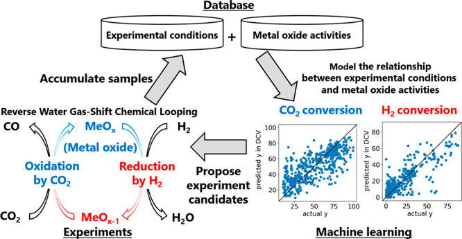
In this study, we focused on the reverse water gas shift–chemical looping (RWGS-CL) reaction.10 The RWGS reaction proceeds via the following two steps that are either spatially or temporally separated via a metal oxide (MOx), which acts as an oxygen carrier
| 2 |
| 3 |
Hence, high CO2 conversion can be achieved owing to low H2O concentration in the second step, which causes an unwanted backward reaction in eq 1. Daza et al.11−13 investigated the effects of Cu and Sr doping on perovskites used as the metal oxide catalyst. Siriwardane et al.14 presented data on conversion for two different coals with a chemical looping oxygen carrier, CuO–Fe2O3–alumina, over a range of conditions, including steam and various levels of reduction of the oxygen carrier. Hare et al.15−17 combined a perovskite with a wide variety of supports, such as CeO2, ZrO2, Al2O3, SiO2, and TiO2, at industrial scale. Maiti et al.18 achieved 100% selectivity of CO generation at low temperature (450–500 °C) using La- and Ca-based perovskite oxides. Sun et al.19 proposed a one-pot method to synthesize dual-function materials that contained a sorbent coupled with a catalyst component. Ramos et al.20 discovered material properties that promote CO2 conversion in a perovskite by doping with Co and Mn. Ma et al.21 presented several Co- and Mn-codoped ferrites for a midtemperature RWGS process. Kellar et al.22 searched for the best metal oxide from a process analysis based on thermodynamic data. Although the RWGS-CL reaction has been actively researched, it remains difficult to control because the reaction involves repeated thermochemical redox cycling, and the CO2 and H2 conversions vary greatly depending on the metal oxide composition and experimental conditions. Therefore, metal oxides with high CO2 and H2 conversions have not yet been developed. The objective of this study was to design metal oxides and simultaneously optimize experimental conditions to satisfy target CO2 and H2 conversion extents.
In conventional development of metal oxides, the next experimental candidate, including metal oxides and experimental conditions, is selected based on the experience and intuition of researchers. For example, if design variables for the RWGS-CL process are assumed to be 5 parameters, such as temperature and reactor size, with 10 candidates assumed for each parameter, and the metal oxides are assumed to have 15 candidates, the total number of combinations is 15 × 105 (= 1 500 000), which requires a large number of experiments and is unrealistic. Therefore, we focused on machine learning to efficiently determine optimal metal oxides for this application. Mathematical models of Y = f(X) were constructed for CO2 and H2 conversions (Y) and descriptors for metal oxides and experimental conditions (X) using experimental results. Y-values were estimated by inputting X-values for metal oxides and experimental conditions into the models. By using models and estimating Y-values, it is possible to realistically handle 1 500 000 combinations of candidates. By selecting the next experimental candidates from estimation results, then an X that leads to target performances can be selected from a huge number of combinations of metal oxides and experimental conditions. In a typical mathematical model, the applicability domain (AD) is set, and candidates with desirable Y-values are selected within the AD. In the case of Gaussian process regression (GPR),23 the candidates considered include variability of the estimated Y-values, called Bayesian optimization.24 AD is useful for reliable prediction of X-values in interpolation regions, while Bayesian optimization is useful for exploring extrapolation in repeated experiments.
In addition to machine learning, we used transfer learning to improve the prediction accuracy of the mathematical models by incorporating a data set and knowledge of oxygen vacancy formation energy (OVFE).
2. Method
2.1. Data
The data comprised 520 samples that were investigated by Sekisui Chemical Co., Ltd. Test measurements were carried out at atmospheric pressure in a quartz tube microreactor, placed in an electric furnace. Typically, 200 mg of sample was packed between quartz wool plugs. First, the samples were heated to 650 °C under He. After this, the samples were reduced for 5 min in 100% H2, flushed for 5 min under He, and then 100% CO2 was flowed for 5 min, followed by another 5 min of He flushing. The total flow rate of the feed gas into the reactor was kept constant at 5.0 mL·min–1. This process was repeated one time for a total of two cycles.
There were 161 metal oxides. Experimental conditions included the metal, molar rates, precipitation method (sol–gel, coprecipitation, or solid phase), sintering temperature, heat-up time, temperature retention time, hydrogen excess, and reaction temperature. The outlet products were analyzed by a gas chromatograph–mass spectrometer (GC/MS). Consumption of H2 and CO2 is connected in that each molecule consumes and provides one oxygen atom. Hence, the molar amount of hydrogen consumption during reduction corresponds with the molar amount of carbon monoxide produced during CO2 reoxidation. Additionally, the CO selectivity was almost 100% in this reaction. Therefore, H2 conversion was calculated from the ratio of the amount of CO produced and the total amount of the inlet of H2.
For the purposes of this paper, the term of the CO2 conversion was taken to mean the instantaneous conversion ratio of CO2 gas to CO. Accordingly, the CO2 conversion was calculated from the ratio of the amount of CO and CO2 produced in 1 min after the starting of the reaction. For this reason, the conversion of CO2 and H2 was not the same. The CO selectivity was almost 100% in all experiments, which was because separating carbon and hydrogen prevents the generation of CH4.
2.2. Descriptor Calculation
Data from the periodic table, Python Materials Genomics (pymatgen),25 and the Materials Project26 were used to represent structural information for the metal oxides. Periodic table data were collected from the Chemistry Handbook and papers27,28 and included atomic mass, electron count, peripheral electron count, atomic radius, ionic radius, ionization energy, electronegativity, work function, and surface energy. Pymatgen includes data for atomic mass, atomic orbitals, atomic radius, boiling point, density of solid, liquid range, melting point, molar volume, thermal conductivity, and electronegativity for metallic elements. The Materials Project data includes energy, energy per atom, volume, formation energy per atom, band gap, and density. Periodic table data and pymatgen descriptors were obtained for each atom, and weighted averages were determined using the molar rates; similarly, Materials Project descriptors were obtained for each metal oxide, and weighted averages determined using the molar rates.
2.3. Regression Model
Partial least-squares (PLS),29 ridge regression (RR),30 least absolute shrinkage and selection operator (LASSO),31 elastic net (EN),32 linear support vector regression (LSVR),33 nonlinear support vector regression (NLSVR), linear Gaussian process regression (LGPR), random forest (RF),34 light gradient boosting machine (light-GBM),35 and GPR methods were used to build the mathematical models.
The prediction accuracy was evaluated by double cross-validation (DCV).36 The sample was first divided by the number of outer folds. One group was used for validation, and the remaining groups were used for cross-validation (CV) (inner folds) to optimize the hyperparameters and then predict the data for validation. This was done for all groups. The prediction accuracy of the mathematical model was evaluated by comparing the actual and predicted Y-values of the outer CV. For comparison, the coefficient of determination (R2DCV), mean absolute error (MAEDCV), and root-mean-square error (RMSEDCV) were used, as respectively given by
| 4 |
| 5 |
| 6 |
where y(i) is the Y-value of the i-th sample, yDCV(i) is the predicted Y-value of i-th sample by DCV, yaverage is the average of the Y-values, and n is the number of samples.
2.4. Transfer Learning
Transfer learning is a method to improve the prediction accuracy and efficient learning of a mathematical model by transferring knowledge from other data. To improve the prediction accuracy of the mathematical model in this study, we used OVFE values, which are considered to be correlated with the extents of CO2 and H2 conversion. OVFE is the energy released when oxygen atoms are released from metal oxides and is typically calculated by density functional theory calculations. In this study, we used the OVFE values of 45 compounds reported by Deml et al.37
In several transfer learning algorithms, we focused on the frustratingly easy domain adaptation,38 which can transfer knowledge by expanding data sets. The expanded data sets XC ∈ R(mA+mB)×(3n+l) and yc ∈ R(mb+mc)×1 are shown as follows
| 7 |
| 8 |
where Xexp ∈ RmA×l is the experimental condition term, XA ∈ RmA×n is the structural information term of the metal oxides from CO2 and H2 conversion data, XB ∈ RmB×n is the structural information term of the metal oxides from OVFE data, yA ∈ RmA×1 is the CO2 or H2 conversion extent, and yB ∈ RmB×1 is the OVFE value. Furthermore, mA is the number of CO2 and H2 conversion samples, mB is number of OVFE samples, l is the number of experimental conditions, and n is the number of structural information variables. Knowledge of the OVFE data was transferred to the CO2 and H2 conversion data by expanding the original data set.
2.5. Inverse Analysis
By inputting candidates for X-values that have not been experienced, Y-values of experimental results can be estimated without the need for experiments. Therefore, metal oxides that have desirable Y-values are expected to be searched with only a small number of experiments by selecting metal oxides based on prediction results.
Candidates for X were generated in three parts: metal oxides, metal molar ratio, and experimental conditions. Some 2300 metal oxides were generated by selecting 3 metals from the 25 metals that have been used in metal oxides for this application. From this, 4707 candidates were generated in 0.01 increments so that the sum of the molar ratios of the three metals was unity. Three types of precipitation method (coprecipitation, sol–gel, and solid-phase) and two types of hydrogen excess condition (hydrogen-deficient and hydrogen-rich) were generated, resulting in a total of six candidates for the experimental conditions. In addition, the sintering temperature was fixed at 700 °C, the heat-up time was fixed at 180 min, the temperature retention time was fixed at 180 min, and the reaction temperature was fixed at 650 °C.
After the estimated Y-values were obtained, the candidates for X were evaluated. If the mathematical model with the highest prediction accuracy was PLS, RR, LASSO, EN, LSVR, NLSVR, RF, or light-GBM, the AD was set, and the X-candidate that had desirable Y-values within the AD was selected. If the mathematical model with the highest prediction accuracy was LGPR or GPR, the X-candidate that had the highest probability of improvement (PI) value, i.e., the probability of exceeding the maximum Y-values in the training data, was selected.
3. Results and Discussion
3.1. Descriptor Calculations
The correlation coefficients between X and Y are shown in Figure 1 after calculating the structural information for the metal oxides. There are no variables that highly correlated with Y. The maximum correlation coefficient was 0.37 for the atomic orbital energy and melting point, as shown in Figure 1(c). In addition, the data set has X variables that are highly correlated with each other, such as sintering temperature, heat-up time, and reaction temperature, shown in Figure 1(a).
Figure 1.

Correlation coefficients between X and Y where X is (a) experimental conditions, (b) periodic table data, (c) pymatgen descriptors, and (d) Materials Project descriptors.
3.2. Regression Analysis
Mathematical models were constructed between the X and Y values calculated in Section 3.1, and each was evaluated by DCV. The number of DCV inner folds was set to 5 and the number of outer folds was set to 161, which was the number of metal oxides. The mathematical models were validated by assuming that they would predict new metal oxides. The DCV-predicted results for each variable set are shown in Table 1. R2DCV in eq 4, MAEDCV in eq 5, and RMSEDCV in eq 6 were calculated for each variable and mathematical model, and the model with the highest prediction accuracy is listed. For both CO2 and H2 conversions, the prediction accuracy using nonlinear regression models was higher than that using linear regression models. GPR gave the best prediction ability, which is attributed to learning of the complex relationships between X and Y by the kernel functions. For CO2 conversion, the GPR model using the experimental conditions, pymatgen descriptors, and Materials Project descriptors had the highest prediction accuracy, with R2DCV of 0.546. It is considered that the prediction accuracy could be improved by adding the electronic information in the pymatgen descriptors and structural information for the metal oxides in the Materials Project descriptors to the GPR model. For H2 conversion, the GPR model with X comprising the experimental conditions and pymatgen descriptors had the highest prediction accuracy, with R2DCV of 0.733. H2 conversion seems to depend on the experimental conditions, such as hydrogen excess, metal, and metal composition, because the prediction accuracy was almost identical for each variable.
Table 1. Prediction Accuracies of CO2 and H2 Conversions for Each Model Input.
| CO2 conversion |
H2 conversion |
|||||||
|---|---|---|---|---|---|---|---|---|
| model inputs | method | R2DCV | MAEDCV | RMSEDCV | method | R2DCV | MAEDCV | RMSEDCV |
| periodic table | GPR | 0.433 | 13.990 | 18.286 | GPR | 0.660 | 7.487 | 11.566 |
| pymatgen descriptors | GPR | 0.504 | 13.159 | 17.096 | GPR | 0.733 | 6.683 | 10.233 |
| Materials Project descriptors | GPR | 0.367 | 14.576 | 19.320 | GPR | 0.689 | 7.268 | 11.045 |
| periodic table + pymatgen descriptors | GPR | 0.441 | 13.701 | 18.158 | GPR | 0.713 | 6.888 | 10.626 |
| periodic table + Materials Project descriptors | GPR | 0.506 | 12.685 | 17.072 | GPR | 0.697 | 7.253 | 10.908 |
| pymatgen + Materials Project descriptors | GPR | 0.546 | 12.445 | 16.359 | GPR | 0.714 | 7.092 | 10.604 |
| all | RF | 0.542 | 12.397 | 16.428 | RF | 0.682 | 7.676 | 11.186 |
Figure 2 shows plots of the measured and DCV-predicted conversions. Prediction errors were mainly caused by samples in which the metal combination was the same and metal compositions were slightly different, but the conversion changed significantly: for example, the measured CO2 conversion of Cu0.05·Ce0.37·Zr0.57 is 47% and predicted CO2 conversion is 83%; the measured CO2 conversion of Cu0.17·Ce0.33·Zr0.50 is 91%, and predicted is 85%. Y values of other samples could be accurately predicted. The same trend was observed for H2 conversion.
Figure 2.
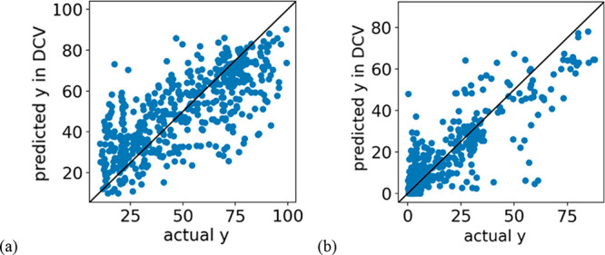
Measured and estimated values of CO2 and H2 conversion by double cross-validation. (a) Y = CO2 conversion, X = experimental conditions, periodic table, and pymatgen descriptors; (b) Y = H2 conversion, X = experimental conditions and pymatgen descriptors.
3.3. Transfer Learning
We conducted transfer learning using the X with the highest accuracy, as determined in Section 3.2. Transfer learning Method 1 added the predicted OVFE values to X; Methods 2 and 3, described in Section 2.4, were used in this study. The method of autoscaling after expanding the data set as per eqs 7 and 8 is defined as Method 2; the method of autoscaling each term, such as Xexp, XA, and XB, before expanding the data set as per eqs 7 and 8 is defined as Method 3.
The OVFE model was first constructed between X, calculated as in Section 2.2, and OVFE and then evaluated for each mathematical model by DCV. The number of DCV inner folds was set to 5 and the number of outer folds was set to 45, which is the number of metal oxides. The mathematical model was constructed as described in Section 2.3. The results of prediction accuracy for each variable by DCV are shown in Table 2. The GPR model between X with the periodic table and pymatgen descriptors and OVFE had the highest prediction accuracy, with R2DCV of 0.886, because there are many variables with a relatively high correlation between OVFE and X, such as atomic mass, solid density, melting point, and boiling point.
Table 2. Prediction Accuracy of Oxygen Vacancy Formation Energy (OVFE) Values for Each Variable.
| model inputs | method | R2DCV | MAEDCV | RMSEDCV |
|---|---|---|---|---|
| periodic table | PLS | 0.555 | 0.677 | 0.882 |
| pymatgen descriptors | GPR | 0.832 | 0.451 | 0.593 |
| Materials Project descriptors | LSVR | 0.840 | 0.398 | 0.530 |
| periodic table + pymatgen descriptors | GPR | 0.886 | 0.335 | 0.446 |
| periodic table + Materials Project descriptors | PLS | 0.830 | 0.422 | 0.546 |
| pymatgen + Materials Project descriptors | GPR | 0.832 | 0.425 | 0.543 |
| all | PLS | 0.852 | 0.393 | 0.510 |
Figures 3 and 4 show the DCV-predicted OVFE. In Figure 3, most samples appear on the diagonal, and thus, the prediction accuracy is quite high. Figure 4 shows is no relationship between CO2 conversion and predicted OVFE values, but metal oxides with predicted OVFE values of 3 to 4 eV tended to have high H2 conversion.
Figure 3.
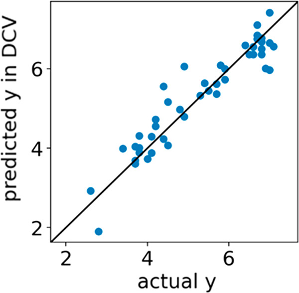
Measured and estimated values of oxygen vacancy formation energy (OVFE) by double cross-validation. y = OVFE, X = periodic table and pymatgen descriptors.
Figure 4.
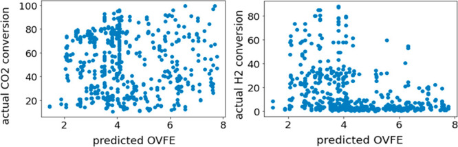
CO2 and H2 conversions and estimated values of oxygen vacancy formation energy (OVFE) by double cross-validation.
We then evaluated the prediction accuracies by DCV for each transfer learning method. The results are shown in Table 3. For both CO2 and H2 conversions, the prediction accuracy was improved by using transfer learning Methods 1, 2, or 3. For CO2 conversion, Method 3 had the highest prediction accuracy. Method 2 was not able to distinguish between the zero matrix and zero with no values; by excepting the zero matrix for autoscaling, Method 3 was able to make this distinction and therefore showed improved prediction accuracy. For H2 conversion, Method 1 had the highest prediction accuracy, because it is considered to reflect a direct relationship between OVFE and H2 conversion.
Table 3. Prediction Accuracy of CO2 and H2 Conversions for Transfer Learning Methods.
| CO2 conversion |
H2 conversion |
|||||||
|---|---|---|---|---|---|---|---|---|
| variable | method | R2DCV | MAEDCV | RMSEDCV | method | R2DCV | MAEDCV | RMSEDCV |
| Section 3.2 | GPR | 0.546 | 12.445 | 16.359 | GPR | 0.733 | 6.683 | 10.233 |
| Method 1 | GPR | 0.550 | 12.428 | 16.290 | GPR | 0.737 | 6.712 | 10.160 |
| Method 2 | GPR | 0.522 | 12.827 | 16.791 | GPR | 0.723 | 6.798 | 10.434 |
| Method 3 | GPR | 0.566 | 12.167 | 16.000 | GPR | 0.730 | 6.771 | 10.296 |
Figure 5 shows the CO2 and H2 conversions with highest DCV-predicted accuracy. Figure 6 shows the feature importance of RF. Comparing Figure 5 with Figure 2, by utilizing knowledge of OVFE, the prediction accuracy is slightly improved in the region where the value of Y is large. In CO2 conversion, the feature importance of XB in eq 7 is high. In Method 2, the feature of XB is not high, and thus, the data set with high feature importance of XB is considered to be suitable for transfer learning. In H2 conversion, the feature importance of the predicted OVFE is high, and this variable may have increased the prediction accuracy.
Figure 5.

Measured and estimated values of CO2 and H2 conversions by double cross-validation using transfer learning. (a) Y = CO2 conversion; transfer learning Method 3; (b) Y = H2 conversion; transfer learning Method 1.
Figure 6.

Random forest feature importance using transfer learning. (a) Y = CO2 conversion; transfer learning Method 3; (b) Y = H2 conversion; transfer learning Method 1.
3.4. Inverse Analysis
We created 65 232 600 candidate metal oxides as described in Section 2.5. The created candidates were input to the regression model with the highest prediction accuracy and the corresponding Y-values predicted. For CO2 conversion, the GPR model was constructed between X, with experimental conditions, pymatgen descriptors, and Materials Project descriptors, and Y using Method 3. For H2 conversion, the GPR model used was constructed between X, with experimental conditions and pymatgen descriptors and Y using Method 1. Figure 7 shows the predicted and experimental Y-values. We were able to find a candidate with predicted Y-values that exceeded the trade-off relationship in the experimental Y-values.
Figure 7.
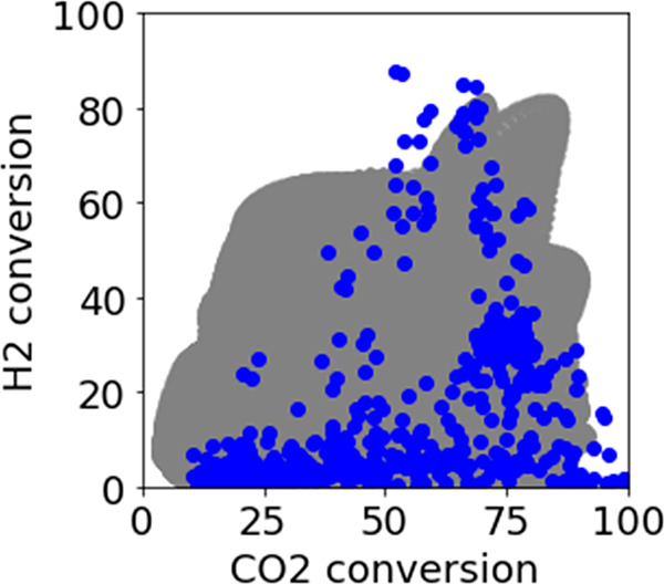
Comparison between experimental (blue) and predicted (gray) Y-values.
Both the CO2 and H2 conversion models used GPR, from which we calculated the PI using the predicted Y-values and their variances. Figure 8 shows the PI values. The 53 red samples are the Pareto optimal solution: six representative samples are shown in Table 4. The Pareto optimal solution is divided into two groups: one with high CO2 conversion and the other with high H2 conversion. Table 4 shows that these values are affected by the hydrogen excess value: when the hydrogen flow is insufficient, the extent of reaction between CO2 and MOx–1 in eq 3 is small because of low reaction between H2 and MOx in eq 2; when the hydrogen flow is excessive, the reaction between CO2 and MOx–1 in eq 3 proceeds well, but the H2 conversion decreases, and thus, PI values for H2 conversion will be low. In Table 5, Cu and Ga, which are known to facilitate high H2 conversion, were selected, and their molar composition was approximately 0.4. From the high RF feature importance shown in Figure 8, the melting point of Cu is larger than that of other metals and the atomic orbitals of both metals are relatively low, accounting for the high CO2 and H2 conversions.
Figure 8.

Probability of improvement (PI) results. Red: Pareto optimal solution (53 samples); gray: all candidates (65 232 600 samples).
Table 4. Samples of Representative Pareto Optimal Solutions.
| metal oxide | log PI [-] | PICO2 [-] | PIH2 [-] | ratio of metal 1 [-] | ratio of metal 2 [-] | ratio of metal 3 [-] | precipitation method | hydrogen excess |
|---|---|---|---|---|---|---|---|---|
| Mg·Cu·Ga | –12.85 | 0.30 | 8.70 × 10⁻⁶ | 0.16 | 0.41 | 0.43 | coprecipitation | excess |
| Mg·Cu·Ga | –12.20 | 0.29 | 1.78 × 10⁻⁵ | 0.18 | 0.48 | 0.34 | coprecipitation | excess |
| K·Cu·Ga | –13.80 | 0.31 | 3.24 × 10⁻⁶ | 0.17 | 0.49 | 0.34 | coprecipitation | excess |
| K·Cu·Ga | –13.93 | 0.32 | 2.84 × 10⁻⁶ | 0.19 | 0.5 | 0.31 | coprecipitation | excess |
| K·Cu·Ga | –2.86 | 0.22 | 0.26 | 0.18 | 0.46 | 0.36 | coprecipitation | less |
| K·Cu·Ga | –2.99 | 0.18 | 0.28 | 0.2 | 0.44 | 0.36 | coprecipitation | less |
Table 5. Samples with the Six Highest Log PI Values.
| metal oxides | log PI [-] | PICO2 [-] | PIH2 [-] | ratio of metal 1 [-] | ratio of metal 2 [-] | ratio of metal 3 [-] | precipitation method | hydrogen excess |
|---|---|---|---|---|---|---|---|---|
| K·Cu·Ga | –2.86 | 0.22 | 0.26 | 0.18 | 0.46 | 0.36 | coprecipitation | less |
| Mg·Cu·Ga | –3.22 | 0.22 | 0.18 | 0.17 | 0.41 | 0.42 | coprecipitation | less |
| Ca·Cu·Ga | –4.02 | 0.18 | 0.10 | 0.17 | 0.38 | 0.45 | coprecipitation | less |
| Cu·Ga·Sr | –4.48 | 0.17 | 0.07 | 0.42 | 0.42 | 0.16 | coprecipitation | less |
| Mn·Cu·Ga | –6.69 | 0.11 | 0.01 | 0.08 | 0.39 | 0.53 | coprecipitation | less |
PI values are probabilities, and therefore, we calculated the probability (log PI) that all Y values exceed the existing Y-values by taking the logarithm for each Y and adding these together. Figure 9 shows the histogram of log PI. Table 5 shows the five metal oxides with highest log PI values. As in Table 4, Cu and Ga were selected; the remaining metals tended to be alkali and alkaline-earth metals, which have a low number of electrons in the outermost electron shell. The state of electrons on the surface of the metal oxide is thought to be important for thermochemical redox cycling to occur. The candidates selected in Tables 4 and 5 were not in the training data. Experiments with the selected candidates are expected to develop metal oxides that exceed the Y-values in the training data set.
Figure 9.
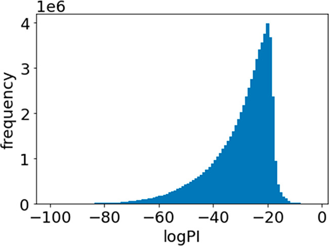
Histogram of logarithm of probability of improvement (log PI).
4. Conclusion
In this study, we constructed mathematical models using machine learning to predict Y-values, where Y is CO2 and H2 conversions. Based on combinations of variables with the highest prediction accuracy and RF (random forest) feature importance, the prediction accuracy for CO2 conversion was improved by adding electronic information and structural information for the metal oxides; H2 conversion seems to depend on experimental conditions, such as hydrogen excess, metal, and metal composition. Furthermore, we focused on OVFE (oxygen vacancy formation energy) values, which are considered to be correlated with the Y-values, and conducted transfer learning. For CO2 conversion, the prediction accuracy was improved by considering the relationship with X; for H2 conversion, which is directly correlated with the predicted OVFE values, the prediction accuracy was improved by using the OVFE values as X. After constructing the mathematical models, we input 65 232 600 candidates as X-values that have not been experienced, and the corresponding Y-values were estimated without experiments. From the predicted Y-values, we were able to find candidates with predicted Y-values that exceed the trade-off relationship in the experimental Y-values. By selecting candidates for the next experiments from the estimated results based on Bayesian optimization and updating the mathematical models with the experimental results, the candidate X metal oxides that will achieve the target Y-values are expected to be found with a small number of experiments.
Although there are lots of experimental results published in the literature regarding CO2 conversion using metal oxides, even when the experimental results are similar in terms of CO2 conversion and metal oxides, the experimental results cannot be compared, the prediction accuracy of models cannot be compared, and the samples cannot be merged if experimental systems and experimental conditions are different. The use of samples from different experimental systems with techniques such as transfer learning would be a challenge for the future.
Acknowledgments
We thank Edanz (https://jp.edanz.com/ac) for editing a draft of this manuscript.
The authors declare no competing financial interest.
Notes
Data and Software Availability: Research data are not shared since experimental data are considered proprietary by the organization and the algorithms of the proposed method are described in the manuscript.
References
- Haszeldine R. S. Carbon Capture and Storage: How Green Can Black Be?. Science 2009, 325 (5948), 1647–1652. 10.1126/science.1172246. [DOI] [PubMed] [Google Scholar]
- Mikkelsen M.; Jorgensen M.; Krebs F. C. The teraton challenge. A review of fixation and transformation of carbon dioxide. Energy Environ. Sci. 2010, 3 (1), 43–81. 10.1039/B912904A. [DOI] [Google Scholar]
- Rao H.; Schmidt L. C.; Bonin J.; Robert M. Visible-light-driven methane formation from CO2 with a molecular iron catalyst. Nature 2017, 548 (7665), 74–77. 10.1038/nature23016. [DOI] [PubMed] [Google Scholar]
- Wang W. H.; Himeda Y.; Muckerman J. T.; Manbeck G. F.; Fujita E. CO2 Hydrogenation to Formate and Methanol as an Alternative to Photo- and Electrochemical CO2 Reduction. Chem. Rev. 2015, 115 (23), 12936–12973. 10.1021/acs.chemrev.5b00197. [DOI] [PubMed] [Google Scholar]
- Wang Y.; Qian Q.; Zhang J. J.; Bediako B. B. A.; Wang Z. P.; Liu H. Z.; Han B. X. Synthesis of higher carboxylic acids from ethers, CO2 and H2. Nat. Commun. 2019, 10, 5395. 10.1038/s41467-019-13463-0. [DOI] [PMC free article] [PubMed] [Google Scholar]
- Daza Y. A.; Kuhn J. N. CO2 conversion by reverse water gas shift catalysis: comparison of catalysts, mechanisms and their consequences for CO2 conversion to liquid fuels. RSC Adv. 2016, 6 (55), 49675–49691. 10.1039/C6RA05414E. [DOI] [Google Scholar]
- Goguet A.; Meunier F. C.; Tibiletti D.; Breen J. P.; Burch R. Spectrokinetic investigation of reverse water-gas-shift reaction intermediates over a Pt/CeO2 catalyst. J. Phys. Chem. B 2004, 108 (52), 20240–20246. 10.1021/jp047242w. [DOI] [Google Scholar]
- Chen C. S.; Cheng W. H.; Lin S. S. Mechanism of CO formation in reverse water-gas shift reaction over Cu/Al2O3 catalyst. Catal. Lett. 2000, 68 (1–2), 45–48. 10.1023/A:1019071117449. [DOI] [Google Scholar]
- Wu H. C.; Chang Y. C.; Wu J. H.; Lin J. H.; Lin I. K.; Chen C. S. Methanation of CO2 and reverse water gas shift reactions on Ni/SiO2 catalysts: the influence of particle size on selectivity and reaction pathway. Catal. Sci. Technol. 2015, 5 (8), 4154–4163. 10.1039/C5CY00667H. [DOI] [Google Scholar]
- Chen X. D.; Chen Y.; Song C. Y.; Ji P. Y.; Wang N. N.; Wang W. L.; Cui L. F. Recent Advances in Supported Metal Catalysts and Oxide Catalysts for the Reverse Water-Gas Shift Reaction. Front. Chem. 2020, 8, 709. 10.3389/fchem.2020.00709. [DOI] [PMC free article] [PubMed] [Google Scholar]
- Daza Y. A.; Kent R. A.; Yung M. M.; Kuhn J. N. Carbon Dioxide Conversion by Reverse Water-Gas Shift Chemical Looping on Perovskite-Type. Oxides Ind. Eng. Chem. Res. 2014, 53 (14), 5828–5837. 10.1021/ie5002185. [DOI] [Google Scholar]
- Daza Y. A.; Maiti D.; Kent R. A.; Bhethanabotla V. R.; Kuhn J. N. Isothermal reverse water gas shift chemical looping on La0.75Sr0.25Co(1-Y)FeYO3 perovskite-type oxides. Catal. Today 2015, 258 (2), 691–698. 10.1016/j.cattod.2014.12.037. [DOI] [Google Scholar]
- Daza Y. A.; Maiti D.; Hare B. J.; Bhethanabotla V. R.; Kuhn J. N. More Cu, more problems: Decreased CO2 conversion ability by Cu-doped La0.75Sr0.25FeO3 perovskite oxides. Surf. Sci. 2016, 648, 92–99. 10.1016/j.susc.2015.11.017. [DOI] [Google Scholar]
- Siriwardane R.; Benincosa W.; Riley J.; Tian H.; Richards G. Investigation of reactions in a fluidized bed reactor during chemical looping combustion of coal/steam with copper oxide-iron oxide-alumina oxygen carrier. Appl. Energy 2016, 183, 1550–1564. 10.1016/j.apenergy.2016.09.045. [DOI] [Google Scholar]
- Hare B. J.; Maiti D.; Daza Y. A.; Bhethanabotla V. R.; Kuhn J. N. Enhanced CO2 Conversion to CO by Silica-Supported Perovskite Oxides at Low Temperatures. ACS Catal. 2018, 8 (4), 3021–3029. 10.1021/acscatal.7b03941. [DOI] [Google Scholar]
- Hare B. J.; Maiti D.; Ramani S.; Ramos A. E.; Bhethanabotla V. R.; Kuhn J. N. Thermochemical conversion of carbon dioxide by reverse water-gas shift chemical looping using supported perovskite oxides. Catal. Today 2019, 323, 225–232. 10.1016/j.cattod.2018.06.002. [DOI] [Google Scholar]
- Hare B. J.; Maiti D.; Meier A. J.; Bhethanabotla B. J.; Kuhn J. N. CO2 Conversion Performance of Perovskite Oxides Designed with Abundant Metals. Ind. Eng. Chem. Res. 2019, 58 (28), 12551–12560. 10.1021/acs.iecr.9b01153. [DOI] [Google Scholar]
- Maiti D.; Hare B. J.; Daza Y. A.; Ramos A. E.; Kuhn J. N.; Bhethanabotla V. R. Earth abundant perovskite oxides for low temperature CO2 conversion. Energy Environ. Sci. 2018, 11 (3), 648–659. 10.1039/C7EE03383D. [DOI] [Google Scholar]
- Sun H. M.; Wang J. WQ.; Zhao J. H.; Shen B. X.; Shi J.; Huang J.; Wu C. F. Dual functional catalytic materials of Ni over Ce-modified CaO sorbents for integrated CO2 capture and conversion. Appl. Catal., B 2019, 244, 63–75. 10.1016/j.apcatb.2018.11.040. [DOI] [Google Scholar]
- Ramos A. E.; Maiti D.; Daza Y. A.; Kuhn J. N.; Bhethanabotla V. R. Co, Fe, and Mn in La-perovskite oxides for low temperature thermochemical CO2 conversion. Catal. Today 2019, 338, 52–59. 10.1016/j.cattod.2019.04.028. [DOI] [Google Scholar]
- Ma L.; Qiu Y.; Li M.; Cui D. X.; Zhang S.; Zeng D. W.; Xiao R. Spinel-Structured Ternary Ferrites as Effective Agents for Chemical Looping CO2 Splitting. Ind. Eng. Chem. Res. 2020, 59 (15), 6924–6930. 10.1021/acs.iecr.9b06799. [DOI] [Google Scholar]
- Keller M.; Otomo J. CO production from CO2 and H2 via the rWGS reaction by thermochemical redox cycling in interconnected fluidized beds. J. CO2 Util. 2020, 40, 101191. 10.1016/j.jcou.2020.101191. [DOI] [Google Scholar]
- Rasmussen C. E.; Nickisch H. Gaussian Processes for Machine Learning (GPML) Toolbox. J. Mach. Learn. Res. 2010, 11, 3011–3015. [Google Scholar]
- Shahriari B.; Swersky K.; Wang Z. Y.; Adams R. P.; de Freitas N. Taking the Human Out of the Loop: A Review of Bayesian Optimization. Proceeding of the IEEE 2016, 104 (1), 148–175. 10.1109/JPROC.2015.2494218. [DOI] [Google Scholar]
- Ong S. P.; Richards W. D.; Jain A.; Hautier G.; Kocher M.; Cholia S.; Gunter D.; Chevrier V. L.; Persson K. A.; Ceder G. Python Materials Genomics (pymatgen): A robust, open-source python library for materials analysis. Comput. Mater. Sci. 2013, 68, 314–319. 10.1016/j.commatsci.2012.10.028. [DOI] [Google Scholar]
- Jain A.; Ong S. P.; Hautier G.; Chen W.; Richards W. D.; Dacek S.; Cholia S.; Gunter D.; Skinner D.; Ceder G.; et al. Commentary: The Materials Project: A materials genome approach to accelerating materials innovation. APL Mater. 2013, 1 (1), 011002 10.1063/1.4812323. [DOI] [Google Scholar]
- Michaelson H. B. The work function of the elements and its periodicity. J. Appl. Phys. 1977, 48 (11), 4729–4733. 10.1063/1.323539. [DOI] [Google Scholar]
- Toyao T.; Suzuki K.; Kikuchi S.; Takakusagi S.; Shimizu K.; Takigawa I. Toward Effective Utilization of Methane: Machine Learning Prediction of Adsorption Energies on Metal Alloys. J. Phys. Chem. C 2018, 122 (15), 8315–8326. 10.1021/acs.jpcc.7b12670. [DOI] [Google Scholar]
- Geladi P.; Kowalski B. R. Partial least-squares regression: A tutorial. Anal. Chim. Acta 1986, 185, 1–17. 10.1016/0003-2670(86)80028-9. [DOI] [Google Scholar]
- Hoerl A. E.; Kennard R. W. Ridge regression: Biased estimation for nonorthogonal problems. Technometrics 1970, 12 (1), 55–68. 10.1080/00401706.1970.10488634. [DOI] [Google Scholar]
- Tibshirani R. Regression shrinkage and selection via the Lasso.. J. R. Stat. Soc. Series B Stat. Methodol. 1996, 58 (1), 267–288. 10.1111/j.2517-6161.1996.tb02080.x. [DOI] [Google Scholar]
- Zou H.; Hastie T. Regularization and variable selection via the elastic net.. J. R. Stat. Soc. Series B Stat. Methodol. 2005, 67 (2), 301–320. 10.1111/j.1467-9868.2005.00503.x. [DOI] [Google Scholar]
- Smola A. J.; Scholkopf B. A tutorial on support vector regression. Stat. Comput. 2004, 14 (3), 199–222. 10.1023/B:STCO.0000035301.49549.88. [DOI] [Google Scholar]
- Breiman L. Random forests. Mach. Learn. 2001, 45 (1), 5–32. 10.1023/A:1010933404324. [DOI] [Google Scholar]
- Ke G.; Meng Q.; Finley T.; Wang T.; Chen W.; Ma W.; Ye Q.; Liu T. Y. LightGBM: A Highly Efficient Gradient Boosting Decision Tree. NIPS 2017, 1–9. [Google Scholar]
- Filzmoser P.; Liebmann B.; Varmuza K. Repeated double cross validation. J. Chemom. 2009, 23 (4), 160–171. 10.1002/cem.1225. [DOI] [Google Scholar]
- Deml A. M.; Holder A. M.; O’Hayre R. P.; Musgrave C. B.; Stevanović V. Intrinsic Material Properties Dictating Oxygen Vacancy Formation Energetics in Metal Oxides. J. Phys. Chem. Lett. 2015, 6 (10), 1948–1953. 10.1021/acs.jpclett.5b00710. [DOI] [PubMed] [Google Scholar]
- Daume III H.Frustratingly Easy Domain Adaptation. arXiv, 2009. arXiv:0907.1815 [cs.LG].