Abstract
Endoscopic optical coherence tomography (OCT) imaging offers a non-invasive way to detect esophageal lesions on the microscopic scale, which is of clinical potential in the early diagnosis and treatment of esophageal cancers. Recent studies focused on applying deep learning-based methods in esophageal OCT image analysis and achieved promising results, which require a large data size. However, traditional data augmentation techniques generate samples that are highly correlated and sometimes far from reality, which may not lead to a satisfied trained model. In this paper, we proposed an adversarial learned variational autoencoder (AL-VAE) to generate high-quality esophageal OCT samples. The AL-VAE combines the generative adversarial network (GAN) and variational autoencoder (VAE) in a simple yet effective way, which preserves the advantages of VAEs, such as stable training and nice latent manifold, and requires no extra discriminators. Experimental results verified the proposed method achieved better image quality in generating esophageal OCT images when compared with the state-of-the-art image synthesis network, and its potential in improving deep learning model performance was also evaluated by esophagus segmentation.
1. Introduction
Esophageal diseases are receiving wide attention due to their increasing incidence [1,2]. Optical coherence tomography (OCT) is a non-invasive method that can provide high resolution cross-sectional images of biological tissue on a microscopic scale [1]. By combining the endoscopic probe, endoscopic OCT is able to detect morphological changes caused by esophageal lesions, which can be used as diagnostic information for esophagus diseases [3]. In general, the healthy esophageal wall has clear layered structures, while the pathological esophagus often shows abnormalities such as layer missing or a growth of thickness [4]. As a result, esophagus diseases have the potential to be automatically diagnosed by segmenting and analyzing OCT images [5,6].
Recent studies have shown that deep learning is a particularly powerful tool that has been successfully applied to a wide range of medical imaging tasks [7–10]. Several attempts have been made to introduce the deep learning technique to the field of esophageal OCT image analysis and demonstrated its advantages over traditional approaches [5,6,11]. However, the application of deep learning in clinical is limited since it requires a large number of data to train the network with millions of parameters. A conventional method to alleviate this problem is using data augmentation techniques such as cropping, rotation, elastic deformations to obtain a larger data set [12]. However, these methods operate randomly and generate highly correlated images [13]. Furthermore, such techniques work on the whole image, which may lead to a missing of global topology information of the input. For instance, the elastic deformations may lead to sharply changed tissue boundaries that corrupted the layered structure, which is rare in the real case even on diseased esophagus. These problems lead to unrealistic esophageal OCT samples containing unreasonable features, which may not be an ideal way to augment the data set.
In recent years, increasing studies adopted generative models for medical image augmentation and achieved promising results [13–16]. Among these studies, the variational autoencoders (VAE) [17] and generative adversarial networks (GAN) [18] are two prominent models, whose advantages and limitations are obvious when compared with each other. The VAE is easy to train, but the generated image may be blurry and lack details [19]. On the contrary, the GAN is able to generate more realistic images but the network is difficult to optimize [20,21]. Several approaches have been proposed to address these problems. One common method is the coarse-to-fine strategy, which starts with low resolution image generation and gradually increases the image quality. Representative models are LAPGAN [22], StackGAN [23] and PGGAN [24]. These improvements make the GAN more robust to train, but significantly increase the computational complexity. An alternative way is to construct hybrid models that combine VAE and GAN to improve the generation performance of VAE and reduce the training difficulties of GAN. The VAEGAN [19], ALI [25] and BiGAN [26] are typical hybrid generative networks. However, these hybrid models are usually of more complex architectures, which lead to more parameters and increase the training complexity.
Several studies have reported strategies that use GANs or conditional GANs for OCT image generation. For example, Zha et al. proposed an end-to-end framework for OCT image generation based on the conditional GAN with a new structural similarity index loss, which considers the structure-related details. In experiments, three kinds of retinal disease images were generated and the result is visually appealing [27]. Tavakkoli et al. proposed a GAN-based network to produce fluorescein angiography images from fundus photographs. In their work, a theoretical framework was proposed to establish a shared feature-space between two domains and provides an unrivaled way for the translation of images from one domain to the other [28]. Sun et al. developed a deep-learning method to synthesize polarization-sensitive OCT images by training a GAN [29]. The proposed method has the potential to reduce the cost, complexity, and need for hardware-based imaging systems. It can be found that these methods achieved success in different tasks. However, the unstable training process of GANs and the uncontrollable generation result limits the application of these methods in synthesizing esophageal OCT images.
To alleviate these problems, we proposed a simple yet effective approach to combine the VAE and GAN for synthesizing esophageal OCT images, which is called the adversarially learned VAE (AL-VAE). The AL-VAE is composed of generating and discriminating parts as general GANs to work adversarially. It is implemented by endowing the encoder of the VAE with the ability of a discriminator. In detail, we added an additional loss term to ensure that the encoder can not only learn a representative latent vector, but also distinguish between real and fake samples like a discriminator. As a result, our model does not require an additional discriminator, indicating that the model will not bring about a significant increase in parameter size. In addition, in contrast to the coarse-to-fine strategy, the proposed method generates images in a single stage, resulting in a simpler structure and more efficient training. Our main contributions are summarized as follows:
-
•
We proposed the AL-VAE that combines the VAE and GAN in a simple yet effective way, which does not require additional architectures or extra training processes. Experiments demonstrated that the proposed method outperformed several generative networks in synthesizing esophageal OCT images.
-
•
We investigate the latent vector of the proposed AL-VAE, and experiments demonstrated that the AL-VAE is able to encode the image content, which indicates the artifacts of the esophageal images can be reduced by manipulating the latent vectors.
-
•
We applied the proposed approach as data augmentation to perform esophageal layer segmentation, and results confirmed that the segmentation performance was improved.
The rest of this study is organized as follows. Section 2 describes the related theory and detailed architecture of the proposed AL-VAE. Section 3 describes the experiment, which shows the generation performance of AL-VAE and its potential application in tissue segmentation. Discussions and conclusions are given in Sections 4 and 5, respectively.
2. Material and methods
2.1. Data
The data used in this study were collected in vivo from C57BL mice using an 800 nm ultrahigh resolution (axial resolution m) endoscopic OCT system. The acquired B-scan is able to reveal microscopic structures of the esophagus. The original B-scan is of the size , which was first cut to to focus on the layered structure and then split to four images for the following analysis. All the OCT images were normalized by min-max normalization method to scale the intensity values to [0, 1]. The training set is composed of 10000 images collected from five subjects, and the test set includes 1000 images from another mouse, thus ensuring no overlap between training and testing.
2.2. AL-VAE architecture
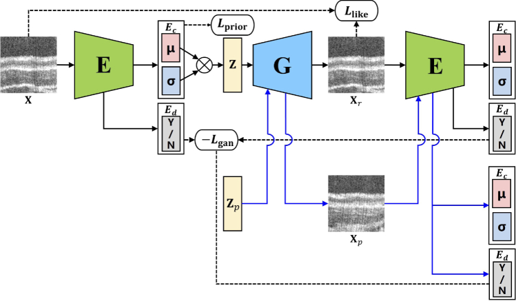
The proposed AL-VAE trains VAE in a self-designed adversarial manner such that the model is able to inherit the advantage of VAEs as well as improve the synthesis performance. The AL-VAE training flow is illustrated in Fig. 1. In this figure, represents the encoder, where denotes the encoding output and represents the discriminative output. is the generator, which also acts as a decoder. is the input original image and denotes the image reconstructed from latent vector . is a vector sampled from the Gaussian distribution, which is of the same size as . The sampled was used to generate a new sample , which is expected to provide more useful information for the model to learn more expressive latent code and synthesize more realistic samples [19]. It can be found that the encoder was designed in a multi-task way that distinguishes between the generated samples and the real data while performing feature learning. Thus, unlike most traditional hybrid models that suffer from complex network architectures, our architecture requires no extra discriminators. Moreover, different from the coarse-to-fine networks, the proposed model can be trained efficiently in a single stage.
Fig. 1.
Training flow of the proposed AL-VAE. It is composed of only one encoder and one generator. The discriminate objective is added to the encoder so that the AL-VAE requires no extra discriminators.
2.3. Loss function
The AL-VAE is supposed to implement encoding and generation tasks, which are related to three losses as shown in Fig. 1. The detailed expression will be presented in the following.
The relationship of the variables in Fig. 1 is formulated as Eq. (1), where the latect vector encoded from real image is subject to the distribution , and the reconstructed from by the generator is subject to distribution .
| (1) |
For the encoding task, the cost function is shown by Eq. (2),
| (2) |
where
| (3) |
| (4) |
In this case, measures the similarity between the input image and the reconstructed image , while represents the distance between the latent distribution and the prior Gaussian distribution . represents the expection operator and indicates the Kullback-Leibler (KL) divergence. In real implementation, was calculated by Eq. (5), where and indicate the reconstructed image tensor and the real image tensor of the -th batch. represents the Frobenius norm.
| (5) |
The cost function for the adversarial task is formulated in Eq. (6), which indicates the discrimination part of the network is supposed to distinguish the real samples from two kinds of generated samples ( and ), thus achieving more informative latent codes and generating more realistic OCT images.
| (6) |
2.4. Training strategy
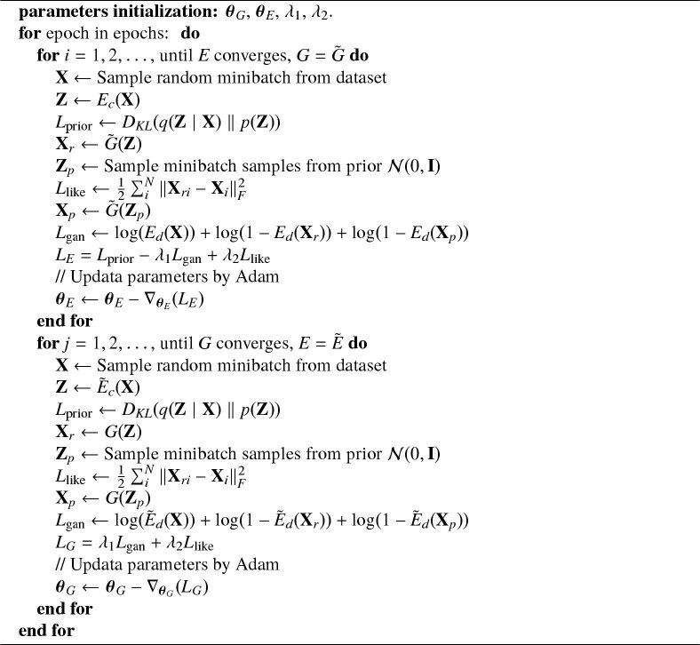
The proposed AL-VAE is an adversarial model, where the encoder and generator within the network are trained alternatively. The three learning objectives of the encoder in this study are: 1) the approximate posterior matches the prior ; 2) low reconstruction error of ; 3) the ability to distinguish between real and generated samples. Accordingly, the loss function of the encoder consisting of three parts for the fixed generator is expressed as:
| (7) |
, and have been explained in previous sections, and and are hyperparameters to control of weight of different items. The generator is supposed to achieve the following objectives: 1) generate samples that are close to the real data distribution; 2) with high reconstruction accuracy. For a fixed encoder , the loss function for can be defined by Eq. (8).
| (8) |
The detailed training procedure is described by Algorithm 1, where the encoder and generator are trained iteratively until reaching the pre-defined maximum epochs.
Algorithm 1. Training of AL-VAE model for synthesis esophageal OCT images.
3. Experiments
In this section, we first introduce the implementation details of the network, and then we evaluate our model’s synthetic performance by comparing with VAE, VAEGAN and PGGAN. Quantitative evaluation was performed using five metrics as will be discussed in the following. In addition, we select several dimensions in latent space to explore the corresponding feature in real images, and demonstrated the potential of the network in synthesizing images with certain features by manipulating the latent vectors.
3.1. Implementation details of the AL-VAE
The input to the network is esophageal OCT images, the latent dimension is set to be 256 in this work. The hyperparameters and in Eq. (7) and Eq. (8) are set at 0.25 and 0.05. The model was trained on a 12 GB Tesla K80 GPU using CUDA 9.2 with cuDNN v7. The losses were optimized by the Adam optimizer [17] with a fixed learning rate . In each iteration, 10 images are randomly selected from the training set to optimize the model, which is the number of batch size. After going through the whole training set, an epoch is finished. The maximum epoch number is set at 200 in this study.
3.2. Analysis of hyperparameters
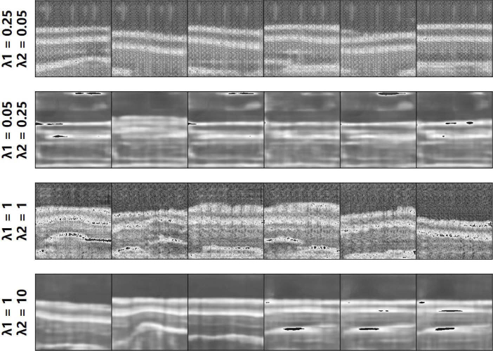
To show the influence of different hyperparameters, we trained the VAE for 40 epochs and use the generation result for an intuitive demonstration. Firstly, we changed the values of and and present the result in Fig. 2. In the first row, and , which is the parameter selected in this study. It can be found the generation result is able to show layer structures, though artifacts exist on the top background. When we swap and in the second row, we can find the generated image is blurry since the reconstruction loss received more attentions due to the larger . In the third row, we set and . The generated result is also of clear layer boundaries. However, dark holes exist in tissues, which may corrupt the topological information. Moreover, the larger and is unfavorable for achieving a nice manifold in the latent space since it weakens the influence of the in Eq. (7). When we changed and , the generated images are blurry for the same reason as the second row, and it is also difficult to achieve latent codes subjected to the predefined distribution.
Fig. 2.
Generation results of AL-VAE with different and values.
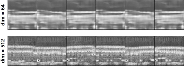
The latent dimension is set at 256 in this study. When we keep and and change the latent dimension to 64 and 512, respectively, the generated images were changed accordingly as shown in Fig. 3. The first row illustrated that the small latent dimension does not capture enough information to generate data with detailed structures, thus producing blurry esophageal images. The second row shows generation results with more clear layer boundaries. However, the relatively large value is unfavorable for selecting meaningful latent code dimensions in the following process. As a result, the dimension is set at 256 in this study.
Fig. 3.
Generation results of AL-VAE with different latent dimensions.
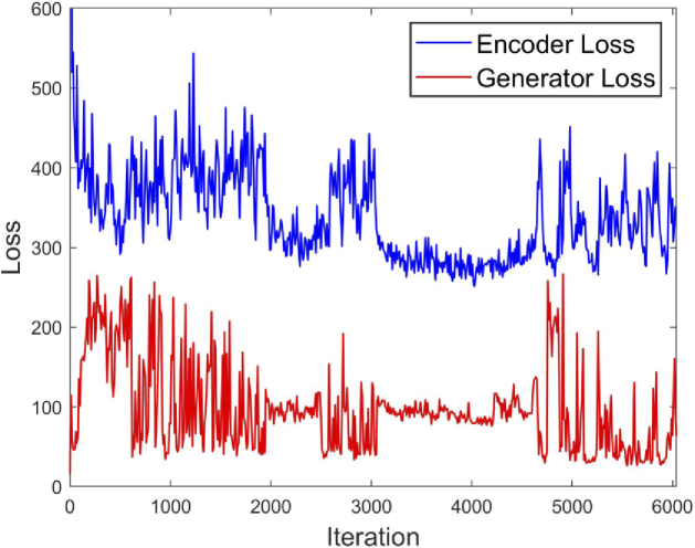
The network is trained in an adversarial way and it is difficult to determine the convergence condition. In Fig. 4, we show the loss curves of 40 epochs with selected parameters ( , , dimension = 256). It can be found that the adversarial loss will become more and more unstable as quality improves. Since a 40-epoch training is able to generate images with primary structures, setting the total training epochs to 200 is enough to achieve satisfactory generation results.
Fig. 4.
Loss curves of the training process of AL-VAE in 40 epochs with , , dimension = 256.
3.3. Results
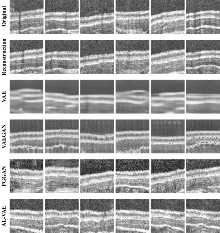
Fig. 5 shows the experiments result of different networks, including the VAE [17], VAEGAN [19], PGGAN [24] and the proposed AL-VAE. The VAE, VAEGAN and AL-VAE were implemented in Pytorch, while the PGGAN is implemented based on a public code [30]. The first row is images sampled from the test set and the reconstruction result by the AL-VAE is shown in the second row. It can be found that the generator is able to reconstruct the input with a clear layered structure, which indicates that the latent vector retains sufficient information of the input image. The generation result of VAE was displayed in the third row. The images show layered structures of the esophageal and even generate the detailed structures of the probe sheath as presented in the last column. However, the image is blurry since VAE is optimized based on element-wise measures like square error. On the contrary, the VAEGAN is able to generate sharper images, but the network is difficult to train due to the extra discriminator. Although we have tried several times, the generated result is still unsatisfactory. For example, the demonstrated images include strange dark points, which are obvious in the last image. The PGGAN and the proposed AL-VAE are able to capture most of the input topological information and provide a clear layered structure of the esophagus. The difference is that the result of our method is of clearer tissues and less noise, which makes the image more realistic in visualization.
Fig. 5.
Demonstration of generation results of different networks. The reconstruction result in the second row is achieved from the AL-VAE.
3.4. Quantitative analysis of the generation result
The following metrics were used to evaluate the quality of the generated images, including the Wasserstein distance (WD) [31], mode score (MS) [32] and the maximum mean discrepancy (MMD) [33]. Among these metrics, the WD and MMD measure distances of two distributions in feature space, where a smaller value indicates more close relationship, representing more realistic generation. The MS measurea the reality and diversity of the generated images, where a larger value indicates better results. The three metrics were calculated by Eqs. (9) to (11).
| (9) |
where and represent the data set of real image and generated image, is sample number, and represent the real samples and the generated samples. is a trained discriminator.
| (10) |
where is a constant, denotes the kernel function.
| (11) |
where and represent the prediction probability of the label for samples from real data set and generated data set, respectively.
1000 images respectively generated by different networks were used to evaluate the network performance. Besides, the 1000 images in the test set were regarded as the gold standard. The comparison results were listed in Table 1. It can be found that the gold standard achieved the smallest value in WD and MMD, and the largest value in MS, which indicates the effectiveness of the selected metrics. Moreover, the AL-VAE achieved metric values closest to the gold standard, indicating its outstanding performance in generating esophageal OCT images.
Table 1. Metrics of the images generated by different models.
| Model | Gold-standard | VAE | VAEGAN | PGGAN | AL-VAE |
|---|---|---|---|---|---|
| WD | 0.0750 a | 0.6811 | 0.4217 | 0.1537 | 0.1234 b |
| MMD | 0.1537 a | 1.3623 | 0.8441 | 0.3072 | 0.2465 b |
| MS | 1.2757 a | 0.6415 | 0.8611 | 1.0403 | 1.1519 b |
indicates the best performance,
indicates the performance closest to the gold standard
3.5. Latent space analysis
We also investigated the latent space by linearly interpolating the real image in the latent space. Specifically, we first applied the trained encoders to the test set to calculate their latent vectors and obtain the range of each dimension. Then, the value in a specific dimension was evenly sampled within the allowable range to observe the change of generated images. In this way, we found some latent dimensions encode particular features of the OCT image. Figure 6 illustrates three examples where some known attributes of OCT images are described by the corresponding latent dimensions. Each row of the image represents a latent dimension related to a specific image feature, which includes the esophageal tissue direction, the tissue thickness and the plastic sheaths (introduced from the imaging equipment), respectively. The images vary gradually from left to right verifying the continuity of the latent space. Note that the plastic sheaths adjoining the esophagus are unfavorable for image processing, and our method provides a way to reduce this artifact by manipulating the corresponding latent dimension.
Fig. 6.
Demonstration of three examples that a particular feature encoded by a specific latent dimension. For each row, the leftmost and rightmost are real images in the test set that with the maximum or minimum values of one specific latent dimension, the rest images are reconstructed from the interpolation of the latent vector.
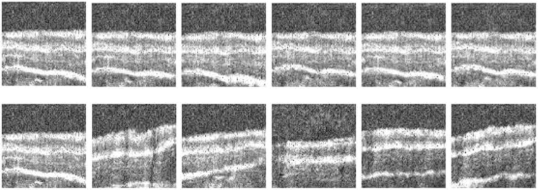
It is also worth mentioning that we have 256 dimensions, but only a few dimensions are ideally disentangled and related to meaningful structures on OCT images. More dimensions are hard to interpret as shown in Fig. 7. The first row presents the situation that the value change in a dimension has little effect on the generated result and the second row shows the generated images did not gradually vary from left to right as the cases in Fig. 6.
Fig. 7.
Demonstration of examples that a specific latent dimension is hard to interpret. For each row, the leftmost and rightmost are real images in the test set that with the maximum or minimum values of one specific latent dimension, the rest images are reconstructed from the interpolation of the latent vector.
3.6. Application in segmentation
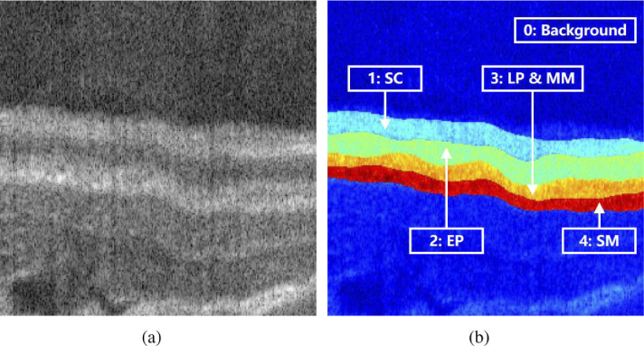
OCT image segmentation is an important technique in computer-aided diagnosis for esophageal disease. A typical task is to recognize different tissues as shown in Fig. 8, where the layers from top to bottom labeled from “1” to “4” are the epithelium stratum corneum (SC), epithelium (EP), lamina propria (LP), muscularis mucosae (MM) and submucosa (SM), respectively.
Fig. 8.
Demonstration of (a) a typical esophageal OCT image for mouse and (b) the corresponding manual segmentation result.
The OCT images generated by AL-VAE can be used to augment the dataset to improve the segmentation performance of the deep network. In the segmentation experiment, we used 800 images from four C57BL mice to construct the training set, and 200 images from two other mice to construct the test set. In comparison, we constructed another training set that was supplemented by 500 samples generated by AL-VAE. In the test set, only real images were included with no generated data.
Traditional data augmentation techniques including random rotation, horizontal flipping, random shearing, elastic deformations were added during training in both of the two cases. The dice similarity coefficients (DSC) are used as evaluation metrics [34] to perform a quantitative evaluation in the test set. The framework of the segmentation model is U-Net [35], which is implemented in Keras using Tensorflow as the backend and trained on a 12 GB Tesla K80 GPU for 100 epochs.
The DSC evaluations for the four target tissue layers (SC, EP, LP MM, SM) in the test set are described as mean standard deviation and listed in Table 2 with the better performance bolded. It can be found that the segmentation model trained by incorporating synthetic data achieved an improvement in DSC values compared to the model using only the real data with traditional augmentation, this suggests that the synthetic data generated by the proposed AL-VAE model are meaningful in practice. These results show that our method may provide the opportunity to train a successful learning model in condition of lacking enough real data for training.
Table 2. DSC evaluation (mean standard deviation) of esophageal layers segmentation. Traditional data augmentation techniques were incorporated during training.
| Methods | SC | EP | LP MM | SM |
|---|---|---|---|---|
| Real data | ||||
| Real + Synthetic |
4. Discussion
We propose an AL-VAE model to synthesize realistic esophageal OCT images by combining GAN and VAE. Benefiting from the adversarial learning in GAN, the proposed model improves the sharpness of VAE result when generating high-quality images. In model training, we add discriminative targets to the encoder, so that the encoder can also be used as a GAN discriminator. This makes our model require no additional architectures compared to traditional hybrid models, thereby reducing the complexity of the model. An extra bonus is that the AL-VAE model can achieve favorable synthetic results in a simple manner with single stage training, rather than processing the image in multiple stages as PGGAN, StackGAN and LAPGAN.
In this paper, the adversarial loss was calculated in the VAE latent space. Using GAN in the latent space has been adopted in adversarial autoencoders (AAE) proposed by Makhzani et al. [36] and their following work PixelGan autoencoder [37]. The AAE used the adversarial training to impose a prior distribution on the latent code to replace the KL divergence penalty of the VAE. As a result, the AAE is able to capture the data manifold better than the VAE. However, the generation result is still blurry [37] since it uses conventional decoders for generation. In contrast, although this study performs adversarial training in the latent space, the adversarial loss was intended to distinguish real images and fake images, which can help produce better generation results.
Section 3.5 shows examples of selected three AL-VAE latent dimensions related with image characteristics. The latent space has not been studied comprehensively in this study since there are also dimensions that seem to be meaningless. Moreover, some dimensions were not disentangled ideally, leading to some specific image characteristics related to a combination of several latent dimensions. However, the experiment in this study still demonstrated the possibilities of the proposed model in generating customized medical images in a controlled manner by manipulating the latent space. In our future work, we will try to develop a method to better disentangle the latent space and search for new latent dimensions that have the potential to manipulate more image characteristics. In that case, images with specific lesions can be synthesized by manipulating a few dimensions of the latent vectors, which is of great significance in clinical. In addition, images from diseased esophagus will also be collected and analyzed to improve the current network.
The proposed network has the potential to remove OCT noise artifacts, which may change the image structure. However, the modification is controlled by the adversarial learning process to generate images approximating the real ones. In that case, the generated images is more suitable to be used than traditional data augmentation techniques that may bring unreasonable changes. It is also worth to mention that the changes will not mess up the quantitative assessment of image quality since we are not simply using the larger or smaller values as the comparison critics. Indeed, we focus more on the comparison with the gold standard, which is the real OCT images independent from the training set. A closer metrics to the gold-standard indicates the generated result is more approximate to a real OCT image.
With additional synthetic data, a better esophageal layer segmentation performance was observed in section 3.6, which suggests that augmenting data with synthetic data generated by our model could help improve supervised learning performance. Researches have shown that insufficient data is a major limitation for automatical image processing method reaching human-level performance. Our previous research solved this problem by focusing on new technologies to implement segmentation tasks with limited training data, such as employing the attention mechanism or multi-stage architectures [5,6]. Experiments showed that they can improve the segmentation result to some extent. In the future, we will try to combine these studies to develop new segmentation models that can process esophagus OCT images comparable to manual segmentation. In addition, the labels of the generated images are manually drawn, which limits its further applications in segmentation tasks. In our future work, the network will be improved to automatically produce masks for the AL-VAE-generated data.
5. Conclusion
In this study, we proposed an AL-VAE model that aims to synthesize realistic esophageal OCT images using an adversarial design for VAE training. To simplify the model architecture, the encoder was designed to implement two tasks: as a conventional encoder to learn expressive latent vectors from the input data set, and as a discriminator to distinguish between real samples and generated samples. Another advantage of AL-VAE is that it retains the advantages of VAE and can train the network robustly and efficiently in a single stage, which alleviates the training difficulties of hybrid models. Experimental results have shown that our model achieved better generation performance when compared with several generartive models. Moreover, the segmentation evaluation results demonstrated that with additional synthesis data, the deep learning based segmentation performance is improved, which indicates our method is effective in data augmentation. For the case with limited dataset, our work may help improve the performance of the deep networks, and it can also be easily extended to other related medical image tasks.
Funding
Natural Science Foundation of Jiangsu Province10.13039/501100004608 (BK20200216); Natural Science Foundation of Shandong Province10.13039/501100007129 (ZR2021QF068, ZR2021QF105).
Disclosures
The authors declare that there are no conflicts of interest related to this article.
Data availability
Data underlying the results presented in this paper are not publicly available at this time but may be obtained from the authors upon reasonable request.
References
- 1.Huang D., Swanson E. A., Lin C. P., Schuman J. S., Stinson W. G., Chang W., Hee M. R., Flotte T., Gregory K., Puliafito C. A., Fujimoto J. G., “Optical coherence tomography,” Science 254(5035), 1178–1181 (1991). 10.1126/science.1957169 [DOI] [PMC free article] [PubMed] [Google Scholar]
- 2.Okuwobi I. P., Ji Z., Fan W., Yuan S. T., Bekalo L., Chen Q., “Automated quantification of hyperreflective foci in SD-OCT with diabetic retinopathy,” IEEE J. Biomed. Health Inform. 24(4), 1125–1136 (2020). 10.1109/JBHI.2019.2929842 [DOI] [PubMed] [Google Scholar]
- 3.Testoni P. A., Mangiavillano B., “Optical coherence tomography in detection of dysplasia and cancer of the gastrointestinal tract and bilio-pancreatic ductal system,” World J. Gastroenterol. 14(42), 6444–6452 (2008). 10.3748/wjg.14.6444 [DOI] [PMC free article] [PubMed] [Google Scholar]
- 4.Gora M. J., Suter M. J., Tearney G. J., Li X. D., “Endoscopic optical coherence tomography: technologies and clinical applications [invited],” Biomed. Opt. Express 8(5), 2405–2444 (2017). 10.1364/BOE.8.002405 [DOI] [PMC free article] [PubMed] [Google Scholar]
- 5.Gan M., Wang C., “Dual-stage u-shape convolutional network for esophageal tissue segmentation in OCT images,” IEEE Access 8, 215020 (2020). 10.1109/ACCESS.2020.3041767 [DOI] [PMC free article] [PubMed] [Google Scholar]
- 6.Wang C., Gan M., “Tissue self-attention network for the segmentation of optical coherence tomography images on the esophagus,” Biomed. Opt. Express 12(5), 2631–2646 (2021). 10.1364/BOE.419809 [DOI] [PMC free article] [PubMed] [Google Scholar]
- 7.Soomro T. A., Afifi A. J., Zheng L. H., Soomro S., Gao J. B., Hellwich O., Paul M., “Deep learning models for retinal blood vessels segmentation: a review,” IEEE Access 7, 71696–71717 (2019). 10.1109/ACCESS.2019.2920616 [DOI] [Google Scholar]
- 8.Sharma H., Jain J. S., Bansal P., Gupta S., “Feature extraction and classification of chest x-ray images using cnn to detect pneumonia,” Proceedings of the Confluence 2020: 10th International Conference on Cloud Computing, Data Science & Engineering pp. 227–231 (2020). [Google Scholar]
- 9.Yamanakkanavar N., Choi J. Y., Lee B., “Mri segmentation and classification of human brain using deep learning for diagnosis of Alzheimer’s disease: A survey,” Sensors 20(11), 3243 (2020). 10.3390/s20113243 [DOI] [PMC free article] [PubMed] [Google Scholar]
- 10.Boveiri H. R., Khayami R., Javidan R., Mehdizadeh A., “Medical image registration using deep neural networks: a comprehensive review,” Comput. Electrical Eng. 87, 106767 (2020). 10.1016/j.compeleceng.2020.106767 [DOI] [Google Scholar]
- 11.Yang Z. Y., Soltanian-Zadeh S., Chu K. K., Zhang H. R., Moussa L., Watts A. E., Shaheen N. J., Wax A., Farsiu S., “Connectivity-based deep learning approach for segmentation of the epithelium in in vivo human esophageal oct images,” Biomed. Opt. Express 12(10), 6326–6340 (2021). 10.1364/BOE.434775 [DOI] [PMC free article] [PubMed] [Google Scholar]
- 12.Milletari F., Navab N., Ahmadi S. A., “V-net: Fully convolutional neural networks for volumetric medical image segmentation,” Proceedings of 2016 Fourth International Conference on 3D Vision (3dv) pp. 565–571 (2016). [Google Scholar]
- 13.Shin H. C., Tenenholtz N. A., Rogers J. K., Schwarz C. G., Senjem M. L., Gunter J. L., Andriole K. P., Michalski M., “Medical image synthesis for data augmentation and anonymization using generative adversarial networks,” Simul. Synth. Med. Imaging 11037, 1–11 (2018). [Google Scholar]
- 14.Frid-Adar M., Diamant I., Klang E., Amitai M., Goldberger J., Greenspan H., “Gan-based synthetic medical image augmentation for increased cnn performance in liver lesion classification,” Neurocomputing 321, 321–331 (2018). 10.1016/j.neucom.2018.09.013 [DOI] [Google Scholar]
- 15.Chaudhari P., Agrawal H., Kotecha K., “Data augmentation using mg-gan for improved cancer classification on gene expression data,” Soft Comput. 24(15), 11381–11391 (2020). 10.1007/s00500-019-04602-2 [DOI] [Google Scholar]
- 16.Luo Y., Zhu L. Z., Wan Z. Y., Lu B. L., “Data augmentation for enhancing eeg-based emotion recognition with deep generative models,” J. Neural Eng. 17(5), 056021 (2020). 10.1088/1741-2552/abb580 [DOI] [PubMed] [Google Scholar]
- 17.Kingma D. P., Welling M., “Auto-encoding variational bayes,” in International Conference on Learning Representations (Iclr), (2014). [Google Scholar]
- 18.Goodfellow I. J., Pouget-Abadie J., Mirza M., Xu B., Warde-Farley D., Ozair S., Courville A., Bengio Y., “Generative adversarial nets,” Adv. Neural Inf. Process. Syst. 27 (Nips 2014) 27, 2672–2680 (2014). [Google Scholar]
- 19.Larsen A. B. L., Sonderby S. K., Larochelle H., Winther O., “Autoencoding beyond pixels using a learned similarity metric,” Int. Conf. on Mach. Learn. Vol 48 48 (2016).
- 20.Gulrajani I., Ahmed F., Arjovsky M., Dumoulin V., Courville A., “Improved training of wasserstein gans,” Adv. Neural Inf. Process. Syst. 30 (Nips 2017) 30 (2017).
- 21.Srivastava A., Valkov L., Russell C., Gutmann M. U., Sutton C., “Veegan: Reducing mode collapse in gans using implicit variational learning,” Adv. Neural Inf. Process. Syst. 30 (Nips 2017) 30 (2017).
- 22.Denton E., Chintala S., Szlam A., Fergus R., “Deep generative image models using a laplacian pyramid of adversarial networks,” Adv. Neural Inf. Process. Syst. 28 (Nips 2015) 28 (2015).
- 23.Zhang H., Xu T., Li H. S., Zhang S. T., Wang X. G., Huang X. L., Metaxas D., “Stackgan: Text to photo-realistic image synthesis with stacked generative adversarial networks,” 2017 IEEE International Conference on Computer Vision (Iccv) pp. 5908–5916 (2017). [Google Scholar]
- 24.Karras T., Aila T., Laine S., Lehtinen J., “Progressive growing of gans for improved quality, stability, and variation,” in International Conference on Learning Representations (Iclr), (2018). [Google Scholar]
- 25.Dumoulin V., Belghazi I., Poole B., Mastropietro O., Lamb A., Arjovsky M., Courville A., “Adversarially learned inference,” (2016).
- 26.Donahue J., Krahenbuhl P., Darrell T., “Adversarial feature learning,” in International Conference on Learning Representations (ICLR), (2017). [Google Scholar]
- 27.Zha X. W., Shi F., Ma Y. H., Zhu W. F., Chen X. J., “Generation of retinal OCT images with diseases based on cgan,” Med. Imaging 2019: Image Process 10949 (2019).
- 28.Tavakkoli A., Kamran S. A., Hossain K. F., Zuckerbrod S. L., “A novel deep learning conditional generative adversarial network for producing angiography images from retinal fundus photographs,” Sci. Rep. 10(1), 21580 (2020). 10.1038/s41598-020-78696-2 [DOI] [PMC free article] [PubMed] [Google Scholar]
- 29.Sun Y., Wang J. F., Shi J. D., Boppart S. A., “Synthetic polarization-sensitive optical coherence tomography by deep learning,” npj Digit. Med. 4(1), 105 (2021). 10.1038/s41746-021-00475-8 [DOI] [PMC free article] [PubMed] [Google Scholar]
- 30.Shin M., “A pytorch implementation of pggan,” Website (2019). https://github.com/nashory/pggan-pytorch.
- 31.Panaretos V. M., Zemel Y., “Statistical aspects of Wasserstein distances,” Annu. Rev. Stat. Appl. 6(1), 405–431 (2019). 10.1146/annurev-statistics-030718-104938 [DOI] [Google Scholar]
- 32.Che T., Li Y., Jacob A. P., Bengio Y., Li W., “Mode regularized generative adversarial networks,” (2017).
- 33.Bounliphone W., Belilovsky E., Blaschko M. B., Antonoglou I., Gretton A., “A test of relative similarity for model selection in generative models,” (2016).
- 34.Taha A. A., Hanbury A., “Metrics for evaluating 3D medical image segmentation: analysis, selection, and tool,” BMC Med. Imaging 15(1), 29 (2015). 10.1186/s12880-015-0068-x [DOI] [PMC free article] [PubMed] [Google Scholar]
- 35.Ronneberger O., Fischer P., Brox T., “U-net: convolutional networks for biomedical image segmentation,” Med. Image Comput. Comput. Interv. Pt Iii 9351, 234–241 (2015). [Google Scholar]
- 36.Makhzani A., Shlens J., Jaitly N., Goodfellow I., Frey B., “Adversarial autoencoders,” (2016).
- 37.Makhzani A., Frey B., “Pixelgan autoencoders,” in Advances in Neural Information Processing Systems 30 (Nips 2017), vol. 30 (2017). [Google Scholar]
Associated Data
This section collects any data citations, data availability statements, or supplementary materials included in this article.
Data Availability Statement
Data underlying the results presented in this paper are not publicly available at this time but may be obtained from the authors upon reasonable request.


