Optimal Two-Stage Genotyping in Population-Based Association Studies

Abstract

We propose a cost-effective two-stage approach to investigate gene-disease associations when testing a large number of candidate markers using a case-control design. Under this approach, all the markers are genotyped and tested at stage 1 using a subset of affected cases and unaffected controls, and the most promising markers are genotyped on the remaining individuals and tested using all the individuals at stage 2. The sample size at stage 1 is chosen such that the power to detect the true markers of association is 1−β₁ at significance level α₁. The most promising markers are tested at significance level α₂ at stage 2. In contrast, a one-stage approach would evaluate and test all the markers on all the cases and controls to identify the markers significantly associated with the disease. The goal is to determine the two-stage parameters (α₁, β₁, α₂) that minimize the cost of the study such that the desired overall significance is α and the desired power is close to 1−β, the power of the one-stage approach. We provide analytic formulae to estimate the two-stage parameters. The properties of the two-stage approach are evaluated under various parametric configurations and compared with those of the corresponding one-stage approach. The optimal two-stage procedure does not depend on the signal of the markers associated with the study. Further, when there is a large number of markers, the optimal procedure is not substantially influenced by the total number of markers associated with the disease. The results show that, compared to a one-stage approach, a two-stage procedure typically halves the cost of the study.

INTRODUCTION

Complex diseases are diseases that do not exhibit a simple Mendelian pattern of segregation and are multifactorial in nature. Linkage analyses were used in the past to identify genes associated with Mendelian disorders, based on information obtained from extended families. This approach, however, requires a large number of potential recombination events to localize the disease susceptibility regions to narrow intervals for practical uses such as positional cloning [Boehnke, 1994]. Well-designed population-based association studies are better suited to identify genes associated with complex diseases [Cardon and Bell, 2001; Cardon and Palmer, 2003]. Association studies are commonly carried out using a case-control design, where the candidate markers are genotyped on all cases and controls. The ability to obtain a large number of markers (such as single-nucleotide polymorphisms) on the human genome has accelerated research interests in association studies. These studies are carried out using either a whole-genome approach or the candidate gene approach. Under the whole-genome approach, markers are evenly spaced throughout the genome, and the markers exhibiting a statistically significant association with the disease outcome are identified. On the other hand, the candidate gene approach focuses on specific (candidate) genomic regions that are selected based on a priori hypotheses regarding their role in disease incidence [Tabor et al., 2002]. Thus, the candidate gene approach involves evaluation of fewer markers than the whole-genome approach. In association studies, typically every marker is first genotyped on all cases and controls, and an appropriate test statistic [such as Armitage’s chi-square test for trend; see Sasieni, 1997] is then used to determine the association between every marker and the disease. This one-stage approach, however, is not a cost-effective strategy when testing a large number of markers, because many of the markers can be eliminated early on in the study as being unlikely to be associated with the disease. Two-stage genotyping strategies were shown to be efficient methods for identifying disease loci in linkage analyses [Elston, 1994; Elston et al., 1996]. Under this approach, a sparse scanning of the genome is performed at stage 1 on all individuals to identify candidate regions. Additional markers flanking and in the candidate regions are genotyped on all the individuals at stage 2 to more accurately localize the disease loci. The two-stage procedure approximately halves the cost of the linkage study in comparison with the one-stage procedure alone [Elston et al., 1996]. Two-stage designs were recently shown to be cost-effective for association studies, where at stage 1 all the markers are evaluated on a subset of the individuals, and the most promising markers are then evaluated at stage 2 using additional individuals [Satagopan et al., 2002]. When the principal constraint is the total cost of the study, a rule-of-thumb two-stage design that provides near-optimal power is to evaluate all the markers on approximately 25% of the individuals at stage 1, and then to validate the top 10% of the markers on all remaining individuals at stage 2. This rule-of-thumb two-stage design enables evaluation of 325% more individuals in comparison with a one-stage design, thus resulting in a substantial increase in power to detect the markers associated with the disease.

Often, however, it may be of more interest to design a study with predefined power than with predefined total cost. In this paper, we consider a two-stage design where the required sample size is first calculated corresponding to a one-stage design with a desired power and significance level. Given this sample size, we then focus on determining the two-stage design that minimizes the cost of marker evaluations such that the desired power is attained. We describe the two-stage design for candidate gene association studies using a statistical hypothesis-testing paradigm to identify the markers significantly associated with the disease. We derive the significance level α₁ and the power 1−β₁ for testing all the markers on a subsample at stage 1. Those markers that are significant will then be tested at stage 2 at significance level α_2, using all the individuals. Our goal is to derive the values of α₁, β₁, and α₂ that minimize the total cost of the study, but such that the desired overall significance level is α and the power is close to 1−β (the desired power of the corresponding one-stage approach). The values of α₁ and β₁ determine the size of the subsample to take at stage 1. Using Monte Carlo simulations, we show that near-optimal power can be achieved under a two-stage approach by utilizing only a fraction of the cost of the corresponding one-stage design.

METHODS

We consider evaluating m markers using a case-control design, where the cases and controls are all unrelated persons. Further, we assume that the markers are not in strong linkage disequilibrium with each other, and hence the markers can be considered independent; in other words, we assume that there is only one marker (which could be defined by a haplotype) for each candidate gene. Suppose there are D (<m) disease loci. We assume that for every disease locus there is a marker in complete linkage disequilibrium with that locus. Our goal is to identify at least one of these loci. A one-stage design will proceed by genotyping all the m markers on all available individuals. At every marker locus we will then test the null hypothesis that the marker is not associated with the disease against the alternative hypothesis that the marker is associated with the disease. Let μ denote the “signal” or design effect of the marker being tested. In a case-control design, the allele (or genotype or haplotype) frequencies in cases and controls are compared at every marker locus to determine association between the locus and the binary disease status. Denoting the allele frequencies in the cases and controls as p₁ and p₀, respectively, the null hypothesis tested at a marker locus is given by H₀: p₁=p₀. Let U₁ and U₀, respectively, denote the observed number of cases and controls carrying the allele of interest at the marker locus. Then, using a binomial distribution, the statistic U₁−U₀ has expected value n(p₁−p₀) and variance n[p₁(1−p₁)+p₀(1−p₀)], where n denotes both the number of cases and the number of controls. Therefore, the signal μ can be interpreted as the “design effect” $\left(p_1-p_0\right)/\sqrt{p_1\left(1-p_1\right)+p_0\left(1-p_0\right)}$. The null hypothesis H₀: p₁=p₀ is equivalent H₀: μ=0. Without loss of generality, here we will consider a one-sided alternative hypothesis H_A: μ>0. We make the large sample assumption that our test statistic is normally distributed with variance proportional to the sample size.

ONE-STAGE PROCEDURE

Let α be the desired overall significance level, and 1−β denote the desired power. Let Φ(.) and ϕ(.) denote the cumulative distribution function and probability density function of the standard normal distribution, respectively. We shall use the notation Z_a to denote the 100*a^th percentile of a standard normal distribution, i.e., Φ(Z_a)=a. Suppose we consider a case-control design with equal numbers (n each, say) of cases and controls. Using the Bonferroni correction for testing m independent markers, the sample size of the one-stage design is given by Witte et al. [2000]:

$$n=\frac{1}{{\mu }^2}{\left(Z_{1-\alpha /m}+Z_{1-\beta }\right)}^2.$$ (1)

When there are multiple disease loci (i.e., D>1) with different signals, we consider μ to represent the smallest of the D signals. In other words, n represents the sample size (number of cases and an equal number of controls) required to detect the disease locus with the smallest signal of interest.

Now let T_A denote the cost of recruiting a case-control pair, and let T_G denote the cost of genotyping a single marker on these two individuals (we assume that both T_A and T_G are known to the investigator). Then the cost of this one-stage design, denoted ${\text{T}}_1^{*}$, is given by ${\text{T}}_1^{*}={\text{nT}}_{\text{A}}+{\text{nmT}}_{\text{G}}$. Let ${\text{T}}_1={\text{T}}_1^{*}/{\text{T}}_{\text{G}}$. Further, let R=T_A/T_G denote the cost of recruiting an individual relative to the cost of genotyping a marker on that individual. Then using as units of cost the cost of genotyping a single marker, the cost of the one-stage design is:

$$T_1=nR+nm.$$ (2)

TWO-STAGE PROCEDURE

Consider the following two-stage design. At stage 1, evaluate (i.e., genotype and test) all m markers using n₁ (<n) cases and n₁ controls, where the sample size n₁ is such that the power to detect a disease locus is 1−β₁ at significance level α₁. Let m₁ (<m) denote the number of markers significant at level α₁. At stage 2, genotype these m₁ markers on the remaining n₂=n−n₁ cases and n₂ controls. Test the m₁ markers at significance level α₂, using all individuals. The markers significant at level α₂ will be identified as the disease loci. The cost of the two-stage design is thus ${\text{T}}_2^{*}={\text{nT}}_{\text{A}}+{\text{n}}_1{\text{mT}}_{\text{G}}+{\text{n}}_2{\text{m}}_1{\text{T}}_{\text{G}}$. Denoting ${\text{T}}_2={\text{T}}_2^{*}/{\text{T}}_{\text{G}}$, the cost of the two-stage design, T₂, can be written as:

$$T_2=nR+n_{1}m+n_2{m}_1.$$ (3)

The above two-stage design has similarities to group sequential designs, commonly used in clinical trials [Jennison and Turnbull, 2000]. As in a group sequential design, the decision to evaluate a marker at stage 2 depends on whether the marker exceeds the desired critical value $Z_{1-{\alpha }_1}$ at stage 1. However, here we test multiple markers at every stage.

Let P represent the power to detect a disease locus using the two-stage design. In the absence of any constraint on sample size, the one-stage design will have the maximum power to detect a disease locus, i.e., 1−β>P. Note that since n₁<n and m₁<m, we have T₂<T₁. Hence, if the two-stage design were to provide power close to that of a one-stage design, and if the cost reduction is substantial, then it would be more cost-effective to perform a two-stage design.

The sample size n₁ at stage 1 is given by:

$$n_1=\frac{{\left(Z_{1-{\alpha }_1}+Z_{1-{\beta }_1}\right)}^2}{{\mu }^2}.$$ (4)

The expected number of significant markers at stage 1 is given by:

$$E\left(m_1\right)=(m-D){\alpha }_1+D\left(1-{\beta }_1\right).$$ (5)

This is a mixture of two binomial random variables, since the D disease loci each have a probability 1−β₁ of being selected at stage 1, and the m−D null loci each have probability α₁ of being selected at stage 1. The values (α₁, β₁, α₂) define the two-stage design parameters. Our goal is to estimate the two-stage design parameters that minimize the expected cost T₂, such that the overall significance level of the two-stage procedure is α and the power P is close to 1−β.

A simplifying assumption to derive the overall significance level and power functions is that, under the alternative hypothesis, an observation on a marker from a single individual has a normally distributed outcome with variance 1 and mean μ. This could be a reasonable approximation so long as the sample size (number of cases and controls) is large enough that the test statistic corresponding to each marker has an approximate normal distribution with variance proportional to the sample size. Let (X₁, X₂) denote the test statistics of a marker at stages 1 and 2. Then X₁~N(n₁μ, n₁) and X₂~N(nμ, n). When the marker is not associated with the disease, μ=0. Further, since cases and controls are randomly sampled (i.e., unrelated individuals), the test statistics follow the Markov property, i.e., X₂−X₁ is independent of X₁. Hence, X₂−X₁~N(n₂μ, n₂). In other words, the test statistic pair (X₁, X₂) for a marker in the two stages has a bivariate normal distribution with mean vector (n₁μ, nμ) and covariance matrix $\Sigma =\left(\begin{array}{ll}{n}_1\hfill & n_1\hfill \\ n_1\hfill & n\hfill \end{array}\right)$.

OVERALL SIGNIFICANCE LEVEL AND POWER OF THE TWO-STAGE PROCEDURE

The overall significance α is the probability of finding at least one significant association under the null hypothesis (i.e., at least one false-positive association). Let P₀(.) denote the probability of an event under the null hypothesis. The probability of detecting a false-positive association at stage 1 is ${\alpha }_1=P_0\left(X_1>Z_{1-{\alpha }_1}\sqrt{n_1}\right)$. Let p₂ denote the conditional probability of a false-positive association at stage 2, given there is a false-positive association at stage 1. Then $p_2=P_0\left(X_2>Z_{1-{\alpha }_2}\sqrt{n}\mid X_1>Z_{1-{\alpha }_1}\sqrt{n_1}\right)$. Hence, the overall significance level can be obtained as below:

$$\begin{gathered} 1-\alpha =P_0\left(\mathit{\text{no false positive associations}}\right) \\ =P_0\left(\mathit{\text{no false positive association at Stage}}1\right)+P_0\left(\mathit{\text{at least }}1\mathit{\text{ false positive association at Stage}}1\mathit{\text{ and none at Stage}}2\right) \\ ={\left(1-{\alpha }_1\right)}^m+\sum _{k=1}^m{P}_0\left(\mathit{\text{k false positive associations at Stage}}1\mathit{\text{ and none at Stage}}2\right) \\ ={\left(1-{\alpha }_1\right)}^m+\sum _{k=1}^m\left(\begin{array}{c}m\\ k\end{array}\right){\alpha }_1^k{\left(1-{\alpha }_1\right)}^{m-k}{\left(1-p_2\right)}^k \\ ={\left(1-{\alpha }_1\right)}^m+\sum _{k=1}^m\left(\begin{array}{l}m\hfill \\ k\hfill \end{array}\right){\left(\frac{{\alpha }_1\left(1-p_2\right)}{1-{\alpha }_1}\right)}^k{\left(1-{\alpha }_1\right)}^m \\ =\sum _{k=0}^m\left(\begin{array}{l}m\hfill \\ k\hfill \end{array}\right){\left(\frac{{\alpha }_1\left(1-p_2\right)}{1-{\alpha }_1}\right)}^k{\left(1-{\alpha }_1\right)}^m \\ ={\left(1-{\alpha }_1{p}_2\right)}^m. \end{gathered}$$

When the total number of markers m is large, we have $\alpha /m={\alpha }_1{p}_2=P_0\left(X_1>Z_{1-{\alpha }_1}\sqrt{n_1},X_2>Z_{1-{\alpha }_2}\sqrt{n}\right)$.

The power P of the two-stage procedure is the probability of selecting a disease locus under the alternative hypothesis. Therefore, denoting P_A(.) as the probability of an event under the alternative hypothesis, we can write P as follows:

$$\begin{gathered} P=P_A\left(X_1>Z_{1-{\alpha }_1}\sqrt{n_1},X_2>Z_{1-{\alpha }_2}\sqrt{n}\right) \\ ={\int }_{Z_{1-{\alpha }_1}}^{\infty }\left[1-\Phi \left(\frac{Z_{1-{\alpha }_2}\sqrt{n}-z\sqrt{n_1}-n_2\mu }{\sqrt{n_2}}\right)\right]\times \varphi \left(z-\mu \sqrt{n_1}\right)dz. \end{gathered}$$ (6)

The right hand side of this equation is an increasing function of α₂ for given values of m, μ, α, β (and hence n), α₁, and β₁ (and hence n₁). The significance level can be obtained from Equation (6) by setting μ=0.

ESTIMATING THE TWO-STAGE DESIGN PARAMETERS

The expected cost function of the two-stage approach is given by T₂ = nR + n₁m + (n − n₁)E(m₁). This expected cost function is, therefore, a function of α₁ and β₁, and using this and Equations 4 and 5 we can write:

$$\left(T_2-nR\right){\mu }^2=m{\left(Z_{1-{\alpha }_1}+Z_{1-{\beta }_1}\right)}^2+\left[(m-D){\alpha }_1+D\left(1-{\beta }_1\right)\right]\times \left[{\left(Z_{1-\alpha /m}+Z_{1-\beta }\right)}^2-{\left(Z_{1-{\alpha }_1}+Z_{1-{\beta }_1}\right)}^2\right].$$ (7)

Our goal is to minimize the expected cost given by Equation (7) with respect to the three unknowns (α₁, β₁, α₂), subject to the significance level and power constraints given by Equation 6, for given values of m, D, R, μ, α, and β (and hence of n). More specifically, our goal is to estimate the value of the parameters (α₁, β₁, α₂) that provide the minimum cost, such that the power P of the two-stage design is close to 1−β, the power of the one-stage design. In other words, for a given small positive value of ϵ, the estimated parameters must be such that (1−β)−P≤ϵ. Minimizing the expected cost T₂ with respect to (α₁, β₁, α₂) is equivalent to minimizing the right-hand side of Equation (7), which is independent of μ and R. Further, it can be easily seen using Equations (1) and (4) that the integrand of Equation (6) is independent of μ when written as functions of α, β, α₁, β₁, and α₂. Hence, the values of (α₁, β₁, α₂) that minimize the expected cost will not depend upon μ or R. When the value of T₂ is specified, the Power Equation 6, the significance-level equation obtained by setting μ=0 in Equation 6, and the Cost Equation (7) constitute three equations in the three unknowns. Hence, a solution to the unknown parameters can be obtained by solving the three equations. Note that when T₂ is specified, β₁ can be estimated from Equation (7) using the Newton-Raphson method for a given α₁. The value of α₂ can then be estimated from Equation (6) by setting μ=0 using the Newton-Raphson method and numerical integration. Finally, P can be calculated from Equation (6) using numerical integration.

The cost fraction (T₂ − nR)/(T₁ − nR) ∈ (0, 1) represents the fraction of marker evaluations performed under the two-stage procedure relative to the one-stage approach. The cost of the one-stage procedure T₁ is known when the values of m, μ, α, β (and hence n), and R are given. Therefore, specifying the cost fraction is equivalent to specifying the (expected) cost T₂ of the two-stage procedure. Further, the significance level for testing at stage 1 is between 0 and 1, i.e., α₁∈(0, 1). We use a Monte Carlo grid search on the unit square to obtain the required solution for given values of m, μ, D, R, α, and 1−β. Every point on the grid corresponds to a value of the cost fraction and α₁. At every point on the grid, we can solve for β₁, α₂, and P as described above. For every cost fraction, we then identify the parameters (α₁, β₁, α₂) where the power P is maximum. Finally, we identify the smallest cost fraction, and hence the minimum expected cost T₂, at which the maximum power P is such that (1−β)−P≤ϵ, for some prespecified ϵ (we take ϵ=0.01). The corresponding values of (α₁, β₁, α₂) provide the required solution.

RESULTS

We calculated the optimal design parameters using Monte Carlo simulations for various combinations of the following parameters: m=25, 50, 100, 200, 500, and 1,000 markers; D=1, 5, and 10 disease loci; overall significance level α=0.01, 0.05; and power of the one-stage design 1−β=0.80, 0.90. Further, we set ϵ=0.01. Therefore, the two-stage procedure is said to have near-optimal power when (1−β)−P≤ϵ.

Figure 1 illustrates the results for D=1, α=0.05 and 1−β=0.80. The horizontal axis shows the cost fraction (shown here between 0.25–0.90). The vertical axis represents the maximum power P of the two-stage procedure. The power is shown for values of m ranging from 25–1,000. The horizontal lines correspond to 1−β=0.80 (power of the one-stage design) and 1−β−ϵ=0.79 (lower bound for achieving near-optimal power). As the cost fraction increases, the power of the two-stage procedure increases towards the power of the one-stage procedure. Note that when the cost fraction increases to one, T₂≈T₁. Therefore, from Equations (2) and (3), nm≈n₁m+n₂m₁=n₁m+(n−n₁)m₁. This implies that m≈m₁. Therefore, when the cost fraction increases to one, the two-stage design is essentially a one-stage design, and hence the power converges to 1−β. Further, for a given cost fraction, the power increases as m increases. The two vertical lines correspond to cost fractions of 50% and 55%. Note that when the cost fraction is above 50%, the power of the two-stage design is between 0.79 and 0.80. In general, when m≥100, the two-stage procedure achieves near-optimal power when the cost fraction is at least 50%.

Fig. 1.

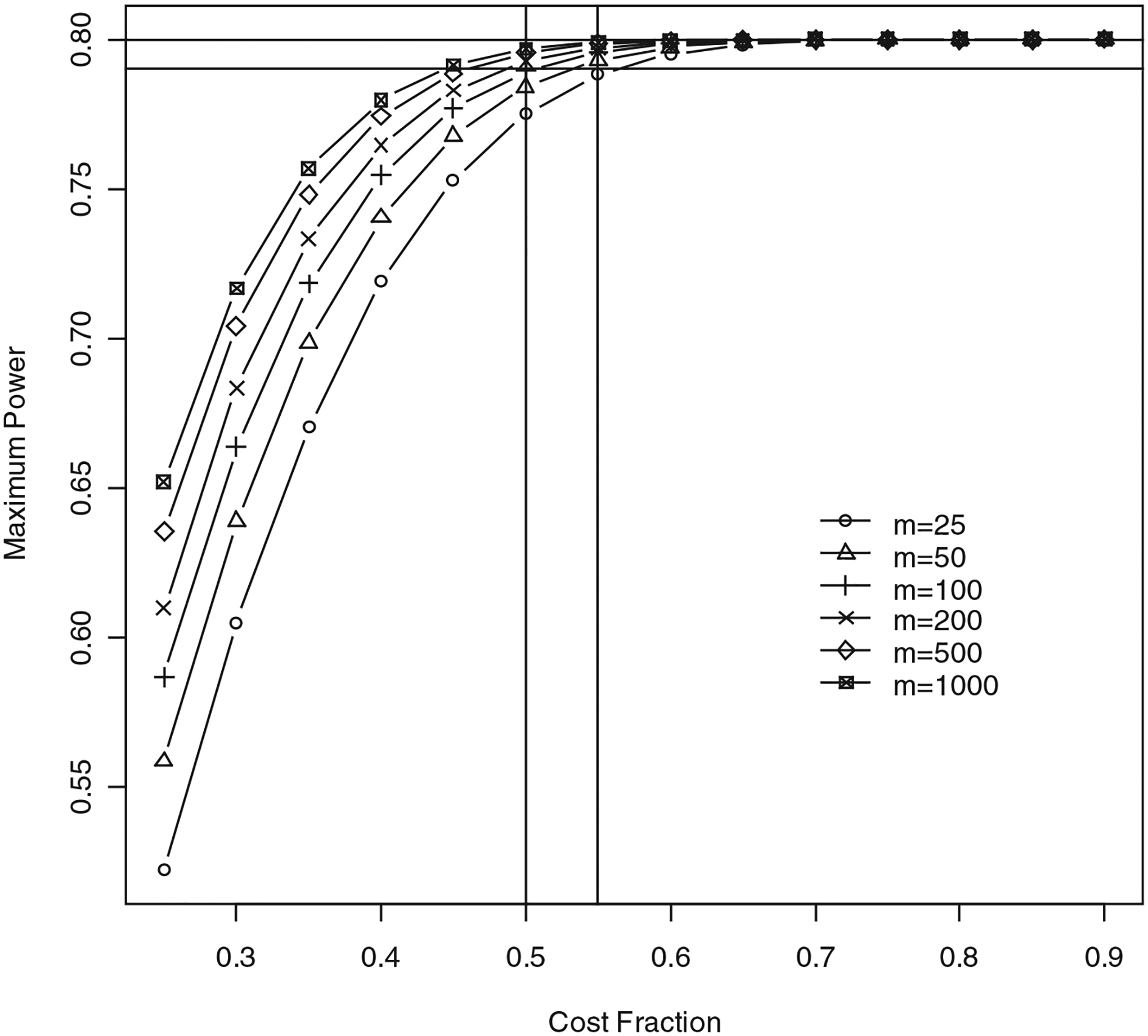
Power of two-stage approach for D=1, α=0.05, 1−β=0.80, and ϵ=0.01. Note that 1−β is power of one-stage approach. Power is shown for values of m ranging from 25–1,000. Horizontal axis shows cost fraction (T₂−nR)/(T₁−nR). Vertical axis shows maximum power attained by two-stage procedure for a given cost fraction. Two horizontal lines correspond to powers of 79% and 80%. Two vertical lines correspond to cost fractions of 50% and 55%.

Tables I–IV illustrate the results of various Monte Carlo simulations. These results show that near-optimal power can be obtained by using only a fraction of the cost of the one-stage procedure. In general, when D=1 and m is large (≥100), a cost fraction of approximately 50% or less is sufficient to obtain near-optimal power. The optimal cost fraction increases as D increases. When m is very large, this increase in the optimal cost fraction is not substantial. For example, when m=1,000, near-optimal power is attained when the cost fraction is approximately 45%, irrespective of the value of D. Similarly, when m=200, near-optimal power is attained when the cost fraction is around 50%. As a general rule-of-thumb, when the number of markers m is large, a judicious choice of two-stage parameters (obtained using Equations 6 and 7) can provide near-optimal power by using only 50% of the cost of a one-stage design. Denoting F as the optimal cost fraction, the optimal expected cost of a two-stage design can be obtained as F × (T₁ − nR) + nR, where n (a function of μ²)is given by Equation (1), and T₁ is given by Equation (2). The value of R is provided by the investigator. For example, let α=0.05, 1−β=0.80, m=100, μ=0.10, R=2, and the cost fraction F=0.50. The sample size is n=1,708, and the expected cost of the two-stage design is 88,816 units.

TABLE I.

Characteristics of optimal two-stage procedure using independent markers, α=0.05, 1−β=0.80, and ϵ=0.01^a

			Optimal parameters
m	D	Optimal cost fraction	α1	β1	α2
25	1	0.56	0.24	0.05	0.002
	5	0.63	0.24	0.05	0.002
50	1	0.43	0.22	0.04	0.001
	5	0.57	0.22	0.04	0.001
100	1	0.51	0.21	0.04	0.0005
	5	0.53	0.21	0.04	0.0005
200	1	0.49	0.19	0.04	0.00026
	5	0.50	0.19	0.04	0.00026
	10	0.51	0.19	0.04	0.00026
500	1	0.46	0.17	0.04	0.0001
	5	0.47	0.17	0.04	0.0001
	10	0.47	0.17	0.04	0.0001
1,000	1	0.45	0.16	0.04	0.00005
	5	0.45	0.16	0.04	0.00005
	10	0.45	0.16	0.04	0.00005

^am, total number of markers; D, number of disease loci.

TABLE IV.

Characteristics of optimal two-stage procedure using independent markers, α=0.01, 1−β=0.90, and ϵ=0.01^a

			Optimal parameters
m	D	Optimal cost fraction	α1	β1	α2
25	1	0.51	0.19	0.03	0.0004
	5	0.59	0.19	0.03	0.0004
50	1	0.48	0.18	0.03	0.0002
	5	0.52	0.18	0.03	0.0002
100	1	0.46	0.17	0.03	0.0001
	5	0.48	0.17	0.03	0.0001
200	1	0.44	0.16	0.03	0.00005
	5	0.45	0.16	0.03	0.00005
	10	0.47	0.16	0.03	0.00005
500	1	0.42	0.14	0.03	0.00002
	5	0.42	0.14	0.03	0.00002
	10	0.43	0.14	0.03	0.00002
1,000	1	0.41	0.13	0.03	0.00001
	5	0.41	0.13	0.03	0.00001
	10	0.41	0.13	0.03	0.00001

^am, total number of markers; D, number of disease loci.

For a given m, the value of D does not (substantially) influence the optimal two-stage parameters. For example, when m=25, α=0.05, and 1−β=0.80, the optimal two-stage parameters are α₁=0.24, β₁=0.05, and α₂=0.002, irrespective of the value of D. This is equivalent to testing all the markers on a subset of n₁ individuals, where n₁ is calculated such that the power to detect a true marker is 1−β₁=95% at α₁=24% significance level at stage 1, and testing the significant markers on all n individuals at α₂=0.2% significance level at stage 2. In general, the optimal value of α₂ is approximately equal to α/m, irrespective of the values of the other parameters. Further, when α=0.05, near-optimal power is attained when the sample size n₁ in stage 1 is chosen such that the power to detect at least one disease locus in stage 1 is approximately 96% (and 97% when α=0.01), irrespective of the values of the other parameters.

DISCUSSION

We have shown that the two-stage procedure is an efficient strategy to identify markers associated with a disease when testing a large number of markers using case-control samples. We can achieve an overall power of 80% using this method by designing the study (i.e., calculating the sample size n) such that the corresponding one-stage design has power 80%+100 × ϵ%, and we suggest setting ϵ=0.01. The optimal two-stage sequential approach derived here, in general, halves the cost (or the number of marker evaluations) of large-scale association studies. Further, our results on the optimal cost fraction are similar to the optimal two-stage procedure for linkage analyses discussed in Elston et al. [1996].

Here we have described two-stage association studies using independent genetic markers. This assumption may be violated when the markers are correlated, e.g., when the markers are in linkage disequilibrium. In particular, when testing every marker individually in an association study, violation of this assumption would influence the overall significance level (given by Equation 6), thus resulting in conservative estimates of significance levels. Note that when multiple single-nucleotide polymorphisms (SNPs) in a candidate gene (or a candidate region) are in complete (or high) linkage disequilibrium, it would be possible to infer their genotypes based on information from one or a few SNPs in that region. Therefore, it would be pragmatic to conduct a pilot study of linkage disequilibrium to first reduce the number of SNPs and only consider a subset of SNPs in a candidate region that represents the biological function of that region, after eliminating SNPs that are in high linkage disequilibrium. The presumption of independent test statistics for the markers would then be reasonable to derive the significance level and power of the two-stage approach in candidate gene association studies.

The two-stage approach proposed here is based on genotyping every marker on all cases and controls (i.e., individual genotyping). DNA pooling is becoming increasingly used as a genotyping strategy for association studies [Shaw et al., 1998]. Under this approach, DNA samples from two or more cases are pooled to create several case DNA pools, and similarly for control DNA pools. Allele frequencies at the marker loci are then obtained using the DNA pools. Ito et al. [2003] suggested DNA pooling using two individuals per pool in order to obtain reliable haplotype information. Wang et al. [2003] evaluated the cost-effectiveness of DNA pooling methods for estimating haplotype frequencies, and recommended using two individuals per DNA pool. DNA pooling enables reduction of genotyping costs, but at the expense of only being able to obtain the allele (or haplotype), rather than genotype, frequencies. The individual genotyping approach, on the other hand, provides complete information on the genotype frequencies of individuals at every marker locus. Testing for deviation from Hardy-Weinberg equilibrium (HWE) proportions in cases was suggested as a more precise method to localize disease loci [Feder et al., 1996; Jiang et al., 2001], provided the mode of inheritance is not multiplicative [Nielsen et al., 1999]. This approach, however, requires knowledge of individual genotype, rather than allele (or haplotype), frequencies. It will be worthwhile to consider a two-stage approach that combines the two genotyping methods. All the markers could be evaluated on a subset of cases and controls at stage 1, using two (or even more) individuals per DNA pool. The most promising markers could then be evaluated on all individuals at stage 2, using individual genotyping so that testing for deviations from HWE could be used to identify causative loci. Two-stage approaches of this type, combining case-control association tests and HWE tests with various genotyping strategies, can be considered. Since, under this approach, controls might only be used in the first stage, the design could focus on ascertaining more cases than controls. Further research is needed to determine cost-efficient strategies of this nature. Finally, it should be noted that, although we focused here on a case-control design where the cases and controls are independent, the same technique can be used when the controls are family-based, such as the pseudosib controls that are used in the transmission/disequilibrium test design [Spielman et al., 1993].

TABLE II.

Characteristics of optimal two-stage procedure using independent markers, α=0.05, 1−β=0.90, and ϵ=0.01^a

			Optimal parameters
m	D	Optimal cost fraction	α1	β1	α2
25	1	0.56	0.23	0.03	0.002
	5	0.63	0.23	0.03	0.002
50	1	0.53	0.22	0.03	0.001
	5	0.56	0.21	0.03	0.001
100	1	0.50	0.19	0.03	0.0005
	5	0.52	0.19	0.03	0.0005
200	1	0.48	0.18	0.03	0.00026
	5	0.49	0.18	0.03	0.00026
	10	0.50	0.18	0.03	0.00026
500	1	0.45	0.16	0.03	0.0001
	5	0.46	0.17	0.03	0.0001
	10	0.46	0.16	0.03	0.0001
1,000	1	0.44	0.16	0.02	0.00005
	5	0.44	0.16	0.02	0.00005
	10	0.44	0.15	0.02	0.00005

^am, total number of markers; D, number of disease loci.

TABLE III.

Characteristics of optimal two-stage procedure using independent markers, α=0.01, 1−β=0.80, and ϵ=0.01^a

			Optimal parameters
m	D	Optimal cost fraction	α1	β1	α2
25	1	0.52	0.20	0.04	0.0004
	5	0.59	0.19	0.04	0.0004
50	1	0.49	0.18	0.04	0.0002
	5	0.53	0.18	0.04	0.0002
100	1	0.47	0.17	0.04	0.0001
	5	0.49	0.17	0.04	0.0001
200	1	0.45	0.16	0.04	0.00005
	5	0.45	0.16	0.04	0.00005
	10	0.47	0.16	0.04	0.00005
500	1	0.43	0.15	0.04	0.00002
	5	0.43	0.15	0.04	0.00002
	10	0.44	0.15	0.04	0.00002
1,000	1	0.41	0.14	0.04	0.00001
	5	0.42	0.14	0.04	0.00001
	10	0.42	0.14	0.04	0.00001

^am, total number of markers; D, number of disease loci.

REFERENCES

- Boehnke M 1994. Limits of resolution of genetic linkage studies: implications for the positional cloning of human genetic diseases. Am J Hum Genet 55:379–390. [PMC free article] [PubMed] [Google Scholar]
- Cardon LR, Bell JI. 2001. Association study designs for complex diseases. Nat Rev Genet 2:91–99. [DOI] [PubMed] [Google Scholar]
- Cardon LR, Palmer LJ. 2003. Population stratification and spurious allelic association. Lancet 361:598–604. [DOI] [PubMed] [Google Scholar]
- Elston RC. 1994. P values, power, and pitfalls in the linkage analysis of psychiatric disorders. In: Gershon ES, Clonings CR, editors. Genetic approaches to mental disorders. Proceedings of the Annual Meeting of the American Psychopathological Association. Washington, DC: American Psychiatric Press. p 3–21. [Google Scholar]
- Elston RC, Guo X, Williams LV. 1996. Two-stage global search designs for linkage analysis using pairs of affected relatives. Genet Epidemiol 13:535–558. [DOI] [PubMed] [Google Scholar]
- Feder JN, Gnirke A, Thomas W, Tsuchihashi Z, Ruddy DA, Basava A, Dormishian F, Domingo R, Ellis MC, Fullan A, Hinton LM, Jones NL, Kimmel BE, Kronmal GS, Lauer P, Lee VK, Loeb DB, Mapa FA, McClelland E, Meyer NC, Mintier GA, Moeller N, Moore T, Morikang E, Prass CE, Quintana L, Starnes SM, Schatzman RC, Brunke KJ, Drayna DT, Risch NJ, Bacon BR, Wolff RK. 1996. A novel MHC class I-like gene is mutated in patients with hereditary haemochromatosis. Nat Genet 13: 399–408. [DOI] [PubMed] [Google Scholar]
- Ito T, Chiku S, Inoue E, Tomita M, Morisaki T, Morisaki H, Kamatani N. 2003. Estimation of haplotype frequencies, linkage-disequilibrium measures, and combination of haplotype copies in each pool by use of pooled DNA data. Am J Hum Genet 72:384–398. [DOI] [PMC free article] [PubMed] [Google Scholar]
- Jennison C, Turnbull BW. 2000. Group sequential methods with applications to clinical trials. New York: Chapman and Hall. [Google Scholar]
- Jiang R, Dong J, Wang D, Sun FZ. 2001. Fine-scale mapping using Hardy-Weinberg disequilibrium. Ann Hum Genet 65:207–219. [DOI] [PubMed] [Google Scholar]
- Nielsen DM, Ehm MG, Weir BS. 1999. Detecting marker-disease association by testing for Hardy-Weinberg disequilibrium at a marker locus. Am J Hum Genet 63:1531–1540. [DOI] [PMC free article] [PubMed] [Google Scholar]
- Sasieni P 1997. From genotypes to genes: doubling the sample space. Biometrics 53:1253–1261. [PubMed] [Google Scholar]
- Satagopan JM, Verbel DA, Venkatraman ES, Offit KE, Begg CB. 2002. Two-stage designs for gene-disease association studies. Biometrics 58:163–170. [DOI] [PMC free article] [PubMed] [Google Scholar]
- Shaw SH, Carrasquillo MM, Kashuk C, Puffenberger EG, Chakravarti A. 1998. Allele frequency distributions in pooled DNA samples: applications to mapping complex disease genes. Genome Res 8:111–123. [DOI] [PubMed] [Google Scholar]
- Spielman RS, McGinnis RE, Ewens WJ. 1993. Transmission test for linkage disequilibrium: the insulin gene region and insulin-dependent diabetes mellitus (IDDM). Am J Hum Genet 52: 506–516. [PMC free article] [PubMed] [Google Scholar]
- Tabor HK, Risch NJ, Myers RM. 2002. Candidate-gene approaches for studying complex genetic traits: practical considerations. Nat Rev Genet 3:1–7. [DOI] [PubMed] [Google Scholar]
- Wang S, Kidd KK, Zhao H. 2003. On the use of DNA pooling to estimate haplotype frequencies. Genet Epidemiol 24:74–82. [DOI] [PubMed] [Google Scholar]
- Witte JS, Elston RC, Cardon LR. 2000. On the relative sample size required for multiple comparisons. Stat Med 19:369–372. [DOI] [PubMed] [Google Scholar]