Think positive: An interpretable neural network for image recognition

Abstract

The COVID-19 pandemic is an ongoing pandemic and is placing additional burden on healthcare systems around the world. Timely and effectively detecting the virus can help to reduce the spread of the disease. Although, RT-PCR is still a gold standard for COVID-19 testing, deep learning models to identify the virus from medical images can also be helpful in certain circumstances. In particular, in situations when patients undergo routine $X$-rays and/or CT-scans tests but within a few days of such tests they develop respiratory complications. Deep learning models can also be used for pre-screening prior to RT-PCR testing. However, the transparency/interpretability of the reasoning process of predictions made by such deep learning models is essential. In this paper, we propose an interpretable deep learning model that uses positive reasoning process to make predictions. We trained and tested our model over the dataset of chest CT-scan images of COVID-19 patients, normal people and pneumonia patients. Our model gives the accuracy, precision, recall and F-score equal to 99.48%, 0.99, 0.99 and 0.99, respectively.

1. Introduction

The pandemic COVID-19 is placing enormous strain on public health systems around the world, and severely affecting the economies of many countries. Although, vaccination is being done for the virus, but the number of the variants of the virus is also increasing. The new variants of the virus can reduce the effectiveness of the vaccines (WHO, 2021). Therefore, along with vaccination for the virus, detection of the virus is important to reduce the spread of the disease and the development of mutants of the virus. In addition to the prevalent testing technique reverse transcription polymerase chain reaction (RT-PCR), deep learning models can also be helpful in efforts to detect the virus. Most of the deep learning algorithms work as a black-box because their reasoning process for their predictions is not transparent/interpretable. However, the interpretation of the reasoning process of a deep learning model related to a high stake decision is important. There have been cases where erroneous data fed into the black-box models went unnoticed, due to which wrongful long prison sentences were given (e.g., inmate Glen Rodriguez was denied parole because of wrong COMPAS score) (Li et al., 2017, Wexler, 2017). The lack of interpretability of the reasoning processes of such deep learning models has become a major issue for whether we can trust predictions that are coming from these models. Therefore, we propose an interpretable deep learning model quasi prototypical part network (Quasi-ProtoPNet), and trained and tested the model over the dataset of chest CT images.

1.1. Related work

In this section, we first discuss those works that are related to our paper because of the interpretability of their reasoning process. Second, we provide a brief summary of the studies that are related to this study as they categorize medical images (chest CT-scan and $X$-ray images). The models in the second category attempt to distinguish medical images of COVID-19 patients from the medical images of pneumonia patients and normal people, but the models are not necessarily interpretable.

Several approaches have emerged to interpret convolutional neural networks, including posthoc interpretability analysis. Once a neural network performs the classification, posthoc analysis is used to interpret the neural network. Deconvolution (Zeiler & Fergus, 2014), saliency visualization (Simonyan et al., 2014, Smilkov et al., 2017, Sundararajan et al., 2017, Wexler, 2017) and activation maximization (Erhan et al., 2009, Hinton, 2012, Lee et al., 2009, Nguyen et al., 2016, Simonyan et al., 2014, Yosinski et al., 2015) are a few examples of posthoc analysis technique. However, these visualization approaches of posthoc analysis do not shed light on the reasoning process with clarity.

Attention-based interpretability is another technique to clarify the reasoning process of the neural networks. The instances of this technique include part-based models (Fu et al., 2017, Girshick et al., 2014, Huang et al., 2015, Ren et al., 2015, Simon and Rodner, 2015, Uijlings et al., 2013, Xiao et al., 2015, Zhang et al., 2014, Zheng et al., 2017, Zhou et al., 2018) and class activation maps (CAM) (Zhou, Khosla, Lapedriza, Oliva, & Torralba, 2016). In this approach, the aim of a model is to show the patches of an input image that are the focus of its attention; nonetheless, these models do not represent prototypes that resemble the parts of an input image that are the focal points of the models. Recently, a model CXR-specific with class activation maps has also been developed to detect COVID-19 from medical images (Rajaraman, Sornapudi, Alderson, Folio, & Antani, 2020).

Case-based classification techniques that use prototypes (Bien and Tibshirani, 2011, Priebe et al., 2003, Wu and Tabak, 2017) or $k$-nearest neighbors (Papernot and McDaniel, 2018, Salakhutdinov and Hinton, 2007, Weinberger and Saul, 2009) are also related to our work. Throughout this paper, a prototype or a prototypical part will represent a patch of an image. Li et al. (2017) have developed a model that uses full image-sized prototypes and requires a decoder for visualizing prototypes. Chen, Li, Barnett, Su, and Rudin (2018) developed a model ProtoPNet which significantly improved on the model developed in Li et al. (2017).

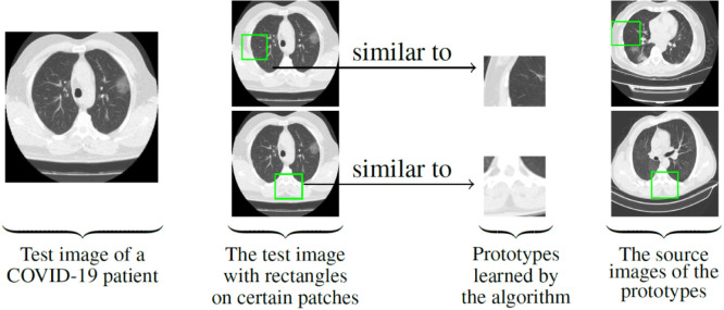
As shown in Fig. 1, ProtoPNet is able to identify different parts of an input image that are similar to different prototypes, and it classifies an image based on the similarity scores. To classify an input image, ProtoPNet finds the Euclidean distance between each latent patch of the input image and the learned prototypes of images from different classes, where prototypes have spatial dimensions 1 × 1. The maximum of the inverted distances between a prototype and the patches of the input image is called the similarity score of the prototype. Note that, the smaller the distance, the larger the reciprocal, and there will be only one similarity score for each prototype. A weighted combination of similarity scores is used to determine the logits for different classes and these logits are normalized using Softmax to determine the class of the input image. The weights for the correct class and incorrect class of a training image are set equal to $1$ and $-0.5$, respectively. These weights are also called connections of the similarity scores with the classes. The negative weights are assigned to include the negative reasoning process, that is, to reject the incorrect classes. ProtoPNet tries to zero out the negative weights during the training process, and with this assumption of ProtoPNet, a theorem is proved (Chen et al., 2018 Theorem 1.1). However, our experiments show that it is hardly possible to zero out the negative connections during the training process after making a negative connection between the similarity scores and incorrect classes.

Fig. 1.

For a given CT-scan image of a COVID-19 patient, Quasi-ProtoPNet identifies the parts of the image where it thinks that this part of the image is similar to that learned prototype.

The models NP-ProtoPNet (Singh & Yow, 2021c), Gen-ProtoPNet (Singh & Yow, 2021a) and Ps-ProtoPNet (Singh & Yow, 2021b) are variations of ProtoPNet, and we refer to these four models collectively the ProtoPNet models or the series of ProtoPNet models. Gen-ProtoPNet model uses a generalized version of the Euclidean distance function, NP-ProtoPNet considers the negative reasoning process and the positive reasoning process but emphasizes on the negative reasoning process, and Ps-ProtoPNet model uses the connections between logits and similarity scores as suggested by Singh and Yow (2021b, Theorem 1), and uses the generalized version of the distance function. The theorem (Singh & Yow, 2021b Theorem 1) uses a more realistic assumption of fixed negative connections between similarity scores and incorrect classes to find the impact of change in the negative connections on the logits. The impact on the logits is obtained due to the projection of prototypes to the patches of training images, that is, the replacement of the prototypes with the latent patches of the training images. However, the use of fixed negative connections leads to decrease in the logit of correct class and increase in the logit of incorrect classes, consequently the accuracy of Ps-ProtoPNet deceases after the projection of prototypes. In particular, the impact is more severe when the number of classes is small, see Singh and Yow (2021b, Theorem 1). In summary, each model of the series of ProtoPNet models uses the negative reasoning process along with the positive reasoning process, whereas our model Quasi-ProtoPNet uses only positive reasoning process to categorize images.

In order to get rid of the flaws of the ProtoPNet models, especially when the number of classes is small, Quasi-ProtoPNet uses only positive reasoning process by placing zero connection between the similarity scores and incorrect classes. Quasi-ProtoPNet suspends the convex optimization of the last layer to keep the connections constant, where by the suspension of the convex optimization of the last layer means that Quasi-ProtoPNet does not optimize the last layer by freezing all other layers. In addition to the positive reasoning process, Quasi-ProtoPNet uses prototypes of all types of spatial dimensions, that is, rectangular spatial dimensions and square spatial dimensions, whereas ProtoPNet model uses the prototypes with only square spatial dimensions 1 × 1. Prototypes with large spatial dimensions help our model to classify the images on the basis of objects instead of backgrounds of the objects in the images. However, the optimum spatial dimensions need to be determined to get better accuracy.

To identify an image that has not been previously exposed, humans can compare patches of the image with patches of images of known objects. This type of reasoning is usually used in difficult identification tasks. For example, radiologists may compare suspicious tumors in an $X$-ray or a CT-scan image with prototype tumor images to diagnose cancer. This type of human reasoning inspired our model where comparison of image parts with learned prototypes is an integral part of the model’s reasoning process. Therefore, our model differentiates between CT-scan images of a COVID-19 patient and CT-scan images of pneumonia patients based on greater similarity between the learned prototypes and the patches of images.

Several non-interpretable networks have been proposed to distinguish chest CT-scan or $X$-ray images of COVID-19 patients from chest CT-scan or $X$-ray images of pneumonia patients and normal people, see Al-Waisy et al., 2020, Al-Waisy et al., 2021, Chaudhary et al., 2021, Chen et al., 2020, Clough et al., 2020, Cohen et al., 2020, Dansana et al., 2020, Gunraj et al., 2021a, Gunraj et al., 2020, Jain, Gupta, et al., 2020, Jain, Mittal, et al., 2020, Kumar et al., 2020, Ozturk et al., 2020, Rajaraman et al., 2020, Reddy et al., 2020 and Zebin and Rezvy (2020). Some studies have surveyed the machine learning/deep learning models that classify chest CT-scan images or $X$-ray images of COVID-19 patients, pneumonia patients and normal people. A survey by Bhattacharya et al. (2021) signifies the lack of sufficient and reliable data of the medical images related COVID-19 patients for neural networks, but a model’s reliability depends data. However, we experimented our model over currently publicly available the biggest dataset of the CT-scan images (Gunraj, Sabri, Koff, & Wong, 2021b). Few more studies (Yan, Gong, et al., 2021, Yan, Hao, et al., 2022, Yan et al., 2020, Yan, Meng, et al., 2022, Yan, Teng, et al., 2021) related to multi-view hashing and image retrieval are also worth mentioning.

1.2. Dataset

We choose the dataset (Gunraj et al., 2021b) of chest CT-scan images of COVID-19 patient, normal people and pneumonia patients to train and test our model. The dataset consists of $143778$ training images and $25658$ test images. We crop the images using the bounding box information provided with the dataset. Also, we use the information provided with the dataset to segregate the cropped images into three classes Covid, Normal and Pneumonia that contain the images of COVID-19 patients, normal people and pneumonia patients, respectively. We also call these classes first, second and third, and denote them by $C,N$ and $P$, respectively. The classes $C,N$ and $P$ have $35996$, $25496$ and $82286$ training images, and $12245$, $7395$ and $6018$ test images, respectively. All images have been resized to the dimensions 224 × 224 as required by the base models.

1.3. Contributions

The novelty of our model is that it uses positive reasoning process along with the use of prototypes that can have any type of spatial dimensions, that is, rectangular spatial dimensions and square spatial dimensions. Quasi-ProtoPNet uses an objective function different from the objective function used in the series of ProtoPNet models. The contributions of this paper are summarized below.

• $•$Quasi-ProtoPNet uses only the positive reasoning process by maintaining zero connection between the similarity scores and incorrect classes. Quasi-ProtoPNet suspends the convex optimization of the last layer to keep the connections fixed. The suspension of the convex optimization also reduces the training time considerably.
• $•$The architecture of Quasi-ProtoPNet helped us to prove a theorem, see Theorem 3.1. The theorem provides the theoretical evidence of the reason of the improvement in the performance of our model over the other ProtoPNet models. We remark that the theorem is not only true for the distance function that we use for our model, but it is also true for any positive-valued function that satisfies the triangular inequality and has appropriate domain.
• $•$Quasi-ProtoPNet uses prototypes with both types of spatial dimensions, that is, rectangular spatial dimensions and square spatial dimensions, whereas ProtoPNet model uses prototypes with only square spatial dimensions 1 × 1.

The rest of the paper is organized as follows. In Section 2, we provide a detailed information about the architecture of our model, and we explain the training procedure and reasoning process of our model. In Section 3, we provide confusion matrices for our model with different base models, and we compare the performance of our model with the ProtoPNet models and the base models. Also, we show that the improvement in the accuracies given by our model over the accuracies given by the other ProroPNet models is statistically significant. A graphical comparison of the accuracies is provided. In this section, we also prove a theorem that finds the bounds of the changes in logits due to projection of prototypes on the training images. In Section 4, we talk about the limitations of our model. In Section 5, a brief discussion on our model and the series of ProtoPNet models is provided. Finally, in Section 6, we conclude our work.

2. Method

In this section, we introduce and explain the architecture and the training process of our model Quasi-ProtoPNet in the context of CT-scan images.

2.1. Quasi-ProtoPNet architecture

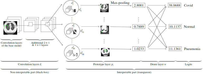
Quasi-ProtPNet can be built on convolutional layers of a state-of-the-art base model (baseline), such as: VGG-19 (Simonyan & Zisserman, 2015), ResNet-34, ResNet-152 (He, Zhang, Ren, & Sun, 2016), DenseNet-121, or DenseNet-161 (Huang, Liu, Van Der Maaten, & Weinberger, 2017). As shown in Fig. 2, Quasi-ProtoPNet consists of the convolution layers of a base model that are followed by two additional convolutional layers 2 × 1 and 1 × 1. These convolutional layers are collectively denoted by $L$, and they are followed by a generalized convolutional layer (Ghiasi-Shirazi, 2019, Nalaie et al., 2017) $p_t$ of prototypical parts. The layer $p_t$ is followed by a dense layer $w$ with no bias. The parameters of $L$ and the weight matrix of a dense layer are denoted by $L_{conv}$ and $w_m$, respectively. The activation functions ReLU and Sigmoid are used for the additional second last convolutional layer and last convolution layer, respectively. Note that, convolutional layers $L$ form a non-interpretable (black-box) part of our model whereas the generalized convolutional layer $p_t$ forms the interpretable (transparent) part of our model.

Fig. 2.

Quasi-ProtoPNet architecture.

Although, convolutional layers of any of the base models can be used to construct our model, we provide the explanation of Quasi-ProtoPNet when it is constructed over the convolutional layers of VGG-$16$. Let $x$ be an input image. Since the output of the convolutional layers of VGG-$16$ has depth $512$ and spatial dimensions 7 × 7, $L\left(x\right)$ has depth $512$ and spatial dimensions 6 × 6. Note that, the layer $p_t$ is a vector of prototypical units, and each prototypical unit is a tensor of the shape $512\times h\times w$, where $1\times 1<h\times w<6\times 6$, that is, $h$ and $w$ together are neither equal to $1$ nor $6$. Suppose $n$ and $m$ denote the total number of classes and prototypes for each class, respectively. Let $P^c={\left\{p_l^c\right\}}_{l=1}^m$ be the set of prototypes of a class $c$ and $P={\left\{P^c\right\}}_{c=1}^n$ is set of all prototypes. For our work $n=3$, but we randomly set the hyperparameter $m=10$.

The shapes of $L\left(x\right)$ and $p_t$ are 512 × 6 × 6 and $512\times h\times w$, where $h$ and $w$ lie between $1$ and $6$ but together they are neither equal to $1$ nor $6$. Therefore, each prototype can be thought of as a part of $L\left(x\right)$. The model takes into account the spatial relationship between $L\left(x\right)$ and the prototypical parts, and upsamples the part of $L\left(x\right)$ (the part of $L\left(x\right)$ that is at the smallest distance from a prototypical part) to the input image $x$ to identify the patch on $x$ that resembles similar to a prototype. The green rectangles in the source images are the parts of the source images from where the prototypes are actually projected. The source image of the prototypes $p_1^1$, $p_1^2$ and $p_{10}^3$ are also shown in Fig. 2. Similar to ProtoPNet (see Section 1.1), Quasi-ProtoPNet computes the similarity scores between an input image and prototypes $p_1^1-p_{10}^1$, $p_1^2-p_{10}^2$ and $p_1^3-p_{10}^3$, see Fig. 2. The prototypes $p_1^1$, $p_1^2$ and $p_{10}^3$ have similarity scores 2.8001, 0.7889 and 1.0233, and the similarity score of $p_1^1$ is greater than the other two similarity scores. The complete list of similarity scores obtained from our experiments is given in the matrix $s_m$, see Section 2.3.

In the dense layer $w$, the matrices $w_m$ and $s_m$ are multiplied to obtain the logits. The logits for the classes $C$, $N$ and $P$ are 38.0688, 10.1137 and 11.1361, respectively. The interpretability/transparency of our model comes into play when an image is classified into a certain class. Our model is able to tell the reason of the classification of the image to that class, and the reason is that the image has some patches more similar to certain learned prototypes related to that class and it shows those learned prototypes. The learned prototypes are projected from the training images, so they are the patches of the training images.

2.2. Training of Quasi-ProtoPNet

Quasi-ProtoPNet uses the generalized version $d$ of the Euclidean distance function, and in this section we show that $d$ is a generalization of the Euclidean distance function. Consider Quasi-ProtoPNet with base model VGG-$16$. Let $x$ be an input image. Therefore, the shape of $L\left(x\right)$ is 512 × 6 × 6 as described in Section 2.1. Let $p$ be any prototype with shape $512\times h\times w$, where $1\le h,w\le 6$, and $h$ and $w$ together are neither equal to $1$ nor $6$. The output $\mathcal{O}(=L\left(x\right))$ of the convolutional layers $L$ has $(7-h)(7-w)$ patches of dimensions $h\times w$. Hence, square of the distance $d({\mathcal{P}}_{ij},p)$ between $p$ and $(i,j)$ patch ${\mathcal{P}}_{ij}$ (say) of $\mathcal{O}$ is:

$$d^2({\mathcal{P}}_{ij},p)=\sum _{l=1}^h\sum _{m=1}^w\sum _{k=1}^{512}{\Vert {\mathcal{O}}_{(i+l-1)(j+m-1)k}-p_{lmk}\Vert }_2^2.$$ (1)

Note that, if $p$ has prototypes of spatial dimensions 1 × 1, that is, $h=w=1$, then $d^2({\mathcal{P}}_{ij},p)={\sum }_{k=1}^{512}{\Vert {\mathcal{O}}_{ijk}-p_{11k}\Vert }_2^2$, which is the square of the Euclidean distance between $p$ and a patch of $\mathcal{O}$, where $p_{11k}\simeq p_k$. Therefore, the function $d$ is a generalization of the Euclidean distance function. The prototypical unit $p_t$ calculates the following.

$$p_t\left(\mathcal{O}\right)=\underset{1\le i\le 7-h,1\le j\le 7-w}{max}log\left(\frac{d^2({\mathcal{P}}_{ij},p)+1}{d^2({\mathcal{P}}_{ij},p)+\epsilon }\right).$$

That is,

$$p_t\left(L\left(x\right)\right)=\underset{\mathcal{P}\in \text{patches}\left(L\left(x\right)\right)}{max}log\left(\frac{d^2(\mathcal{P},p)+1}{d^2(\mathcal{P},p)+\epsilon }\right).$$ (2)

Eq. (2) exhibits that a prototype $p$ is more similar to the image $x$ if the reciprocal of the distance between $p$ and a latent patch of $x$ is smaller. Quasi-ProtoPNet is trained using the following two steps.

2.2.1. Optimization of all layers before the dense layer

Let $X=\{x_1\dots x_n\}$ and $Y=\{y_1\dots y_n\}$ be sets of images and associated labels, respectively, and $D=\{(x_i,y_i):x_i\in X,y_i\in Y\}$. Then our objective function is:

$$\underset{P,L_{conv}}{min}\frac{1}{n}\sum _{i=1}^n\text{CrosEnt}(h\circ p_t\circ L\left(x_i\right),y_i)+\lambda \text{ClstCost},$$ (3)

where ClstCost is given by the equation

$$\text{ClstCost}=\frac{1}{n}\sum _{i=1}^n\underset{j:p_j\in P_{y_i}}{min}\underset{\mathcal{P}\in \text{patches}\left(L\left(x_i\right)\right)}{min}{d}^2(\mathcal{P},p_j).$$ (4)

Eq. (4) discloses that the drop in the cluster cost (ClstCost) leads to the clustering of prototypes around their respective classes. The reduction in cross entropy leads to better classifications, see the objective function (3). The hyperparameter $\lambda$ is set equal to 0.7. Since $w_m$ is the weight matrix for the dense layer, $w_m^{(i,j)}$ is the weight assigned to the connection between logit of $i$th class and similarity score of $j$th prototype. Therefore, for a class $c$, we put $w_m^{(i,j)}=1$ for all $j$ with $p_j^i\in P^i$, and for all $p_j^c⁄\in P^i$ with $c\ne i$, $m_w^{(c,j)}=0$. The non-negativity of the distance function and optimization of all the layers before the last layer with optimizer SGD help Quasi-ProtoPNet to learn important latent spaces.

2.2.2. Projection of prototypes

Let $x$ be an input image. At the second step, Quasi-ProtoPNet projects the prototypes onto the patches of $x$ that are more similar to the prototypes. That is, a patch of $x$ that is at a smaller distance from a prototype gets projected, and the distance must be at least $93$rd percentile of all the inverted distances of the prototype from all the images. For this purpose, Quasi-ProtoPNet makes the following update:

$$p_j^c⟵\text{arg}\underset{\{\mathcal{P}:\mathcal{P}\in \text{patches}\left(L\left(x_i\right)\right)\forall i\text{ such that }{y}_i=c\}}{min}d(\mathcal{P},p_j^c).$$

2.3. Explanation of Quasi-ProtoPNet

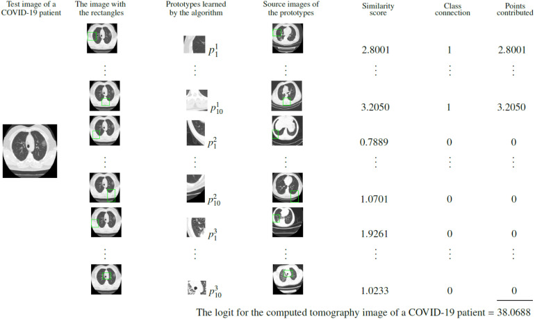
In this section, we explain our model with an example of an input image as given in Fig. 3.

Fig. 3.

The explanation of the reasoning process of the model.

In Fig. 3, the image in the first column belongs to the class Covid. In the second column of the figure, the green rectangle on the image is enclosing the patches of the image that give the highest similarity score to the prototypes in the third column. In the fourth column, the rectangles are enclosing the patches on the source images of the prototypes, that is, the rectangles are pinpointing the patches on the source images from where the prototypes are projected. In the fifth column, similarity scores between the prototypes and patches of the test image are displayed. In the sixth column, the connections between similarity scores and the logits are given. Since the image belongs to the first class $C$, the similarity scores of the prototypes of the second and third class are assigned zero weight. The entries of the seventh column are obtained by multiplying similarity scores and class connections, and the logit (38.0688) for the class $C$ is obtained by adding the entries of the seventh column. The logit for the class $C$ can also be computed by multiplying the first row of $w_m$ with matrix $s_m$. The logits for the classes $N$ and $P$ are 10.1137 and 11.1361, respectively, and can be computed by multiplying second and third row of $w_m$ with matrix $s_m$.

The transpose of the weight matrix $w_m$ and similarity score matrix $s_m$ that we obtain from our experiments are as follows:

$$w_m^T=\left(\begin{array}{ccc}\hfill 1\hfill & \hfill 0\hfill & \hfill 0\hfill \\ \hfill 1\hfill & \hfill 0\hfill & \hfill 0\hfill \\ \hfill 1\hfill & \hfill 0\hfill & \hfill 0\hfill \\ \hfill 1\hfill & \hfill 0\hfill & \hfill 0\hfill \\ \hfill 1\hfill & \hfill 0\hfill & \hfill 0\hfill \\ \hfill 1\hfill & \hfill 0\hfill & \hfill 0\hfill \\ \hfill 1\hfill & \hfill 0\hfill & \hfill 0\hfill \\ \hfill 1\hfill & \hfill 0\hfill & \hfill 0\hfill \\ \hfill 1\hfill & \hfill 0\hfill & \hfill 0\hfill \\ \hfill 1\hfill & \hfill 0\hfill & \hfill 0\hfill \\ \hfill 0\hfill & \hfill 1\hfill & \hfill 0\hfill \\ \hfill 0\hfill & \hfill 1\hfill & \hfill 0\hfill \\ \hfill 0\hfill & \hfill 1\hfill & \hfill 0\hfill \\ \hfill 0\hfill & \hfill 1\hfill & \hfill 0\hfill \\ \hfill 0\hfill & \hfill 1\hfill & \hfill 0\hfill \\ \hfill 0\hfill & \hfill 1\hfill & \hfill 0\hfill \\ \hfill 0\hfill & \hfill 1\hfill & \hfill 0\hfill \\ \hfill 0\hfill & \hfill 1\hfill & \hfill 0\hfill \\ \hfill 0\hfill & \hfill 1\hfill & \hfill 0\hfill \\ \hfill 0\hfill & \hfill 1\hfill & \hfill 0\hfill \\ \hfill 0\hfill & \hfill 0\hfill & \hfill 1\hfill \\ \hfill 0\hfill & \hfill 0\hfill & \hfill 1\hfill \\ \hfill 0\hfill & \hfill 0\hfill & \hfill 1\hfill \\ \hfill 0\hfill & \hfill 0\hfill & \hfill 1\hfill \\ \hfill 0\hfill & \hfill 0\hfill & \hfill 1\hfill \\ \hfill 0\hfill & \hfill 0\hfill & \hfill 1\hfill \\ \hfill 0\hfill & \hfill 0\hfill & \hfill 1\hfill \\ \hfill 0\hfill & \hfill 0\hfill & \hfill 1\hfill \\ \hfill 0\hfill & \hfill 0\hfill & \hfill 1\hfill \\ \hfill 0\hfill & \hfill 0\hfill & \hfill 1\hfill \end{array}\right)\text{and}{s}_m=\left(\begin{array}{c}\hfill 2.8001\hfill \\ \hfill 2.8001\hfill \\ \hfill 2.8001\hfill \\ \hfill 3.2050\hfill \\ \hfill 2.8001\hfill \\ \hfill 1.9548\hfill \\ \hfill 2.4170\hfill \\ \hfill 8.7579\hfill \\ \hfill 7.3285\hfill \\ \hfill 3.2050\hfill \\ \hfill 0.7889\hfill \\ \hfill 1.7505\hfill \\ \hfill 0.7889\hfill \\ \hfill 0.7889\hfill \\ \hfill 1.7363\hfill \\ \hfill 0.8233\hfill \\ \hfill 0.7889\hfill \\ \hfill 0.7889\hfill \\ \hfill 0.7889\hfill \\ \hfill 1.0701\hfill \\ \hfill 1.9261\hfill \\ \hfill 1.0942\hfill \\ \hfill 0.9336\hfill \\ \hfill 0.9524\hfill \\ \hfill 1.0003\hfill \\ \hfill 1.1130\hfill \\ \hfill 0.9112\hfill \\ \hfill 1.0463\hfill \\ \hfill 1.1354\hfill \\ \hfill 1.0233\hfill \end{array}\right).$$

3. Results

In this section, we present the metrics given by our model and compare the performance of our model with the performance of the other models.

3.1. The metrics and confusion matrices

Suppose TP, TN, FP and FN denote the true positives, true negatives, false positives and false negatives for the Covid class. The metrics accuracy, precision, recall and F1-score are (Wikipedia contributors, 2021a, Wikipedia contributors, 2021b, Wikipedia contributors, 2021c):

$$\begin{array}{ccc}\hfill & \hfill \hfill & \text{Accuracy}=\frac{TP+TN}{TP+TN+FP+FN},\text{ Precision}=\frac{TP}{TP+FP}.\hfill \end{array}$$ (5)

$$\begin{array}{ccc}\hfill & \hfill \hfill & \text{Recall}=\frac{TP}{TP+FN},\text{ F1-score}=\frac{2}{{\text{Precision}}^{-1}+{\text{Recall}}^{-1}}.\hfill \end{array}$$ (6)

In Fig. 4, Fig. 5, Fig. 6, Fig. 7, Fig. 8, Fig. 9, the confusion matrices of Quasi-ProtoPNet with the base models are given. For example, in Fig. 4, the confusion matrix $M$ (say) of Quasi-ProtoPNet with baseline VGG-$16$ is provided. Hence, the numbers $M\left[0\right]\left[0\right]$, $M\left[1\right]\left[1\right]+M\left[2\right]\left[2\right]$, $M\left[0\right]\left[1\right]+M\left[0\right]\left[2\right]$ and $M\left[1\right]\left[0\right]+M\left[2\right]\left[0\right]$ are the TP, TN, FP and FN of the class Covid. Therefore, by Eqs. (5), (6), for Quasi-ProtoPNet, the accuracy, precision, recall and F1-score are equal to 99.05, 0.98, 0.99 and 0.98, respectively.

Fig. 4.

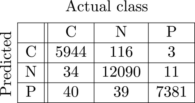
Base VGG-16.

Fig. 5.

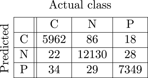
Base VGG-19.

Fig. 6.

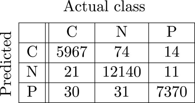
Base ResNet-34.

Fig. 7.

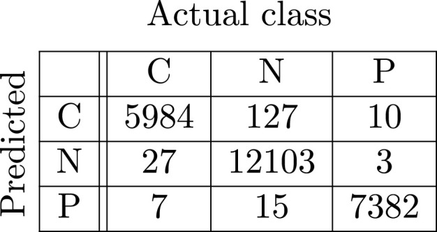
Base ResNet-152.

Fig. 8.

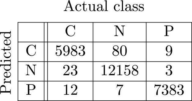
Base DenseNet-121.

Fig. 9.

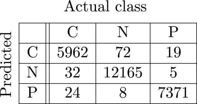
Base DenseNet-161.

3.2. The performance comparison of the models

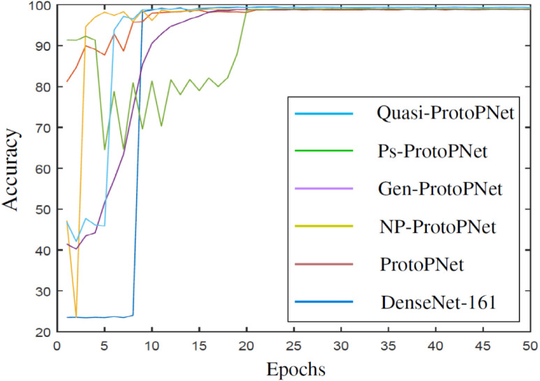
The series of ProtoPNet models are constructed over the convolution layers of the base models. Although, the accuracies of the series of ProtoPNet models and the base models become stabilize prior to $35$ epochs (see Section 3.4), but we trained and tested the models for $100$ epochs.

The performance comparison in the metrics is provided in Table 1. We see from the third column of Table 1 that when we build our model on the convolutional layers of VGG-$16$ then the accuracy, precision, recall and F1-score given by Quasi-ProtoPNet are 99.05, 0.98, 0.99 and 0.98, respectively. The accuracy, precision, recall and F1-score given by the models ProtoPNet, NP-ProtoPNet, Gen-ProtoPNet, Ps-PrortoPNet with base model VGG-$16$, and the base model itself (Base only) are 90.84, 0.89, 0.91 and 0.90; 98.23, 0.93, 0.95 and 0.94; 95.85, 0.93, 0.95 and 0.94; 98.83, 0.96, 0.98 and 0.97; and 99.03, 0.98, 0.99 and 0.98, respectively. The highest accuracies obtained with different base models are in bold. Moreover, we see from the Table 1 that accuracies given by Quasi-ProtoPNet are even better than the accuracies given by the base models when Quasi-ProtoPNet is constructed over the convolutional layers of VGG-$16$, VGG-$19$ and DenseNet-$121$. Furthermore, the highest accuracy (99.48%) achieved by Quasi-ProtoPNet with base model DenseNet-$121$ is equal to the highest accuracy (99.48%) achieved by the non-interpretable model DenseNet-$161$.

Table 1.

The comparison of performances of the models while experimented over the dataset of CT images.

Base	Metric	Quasi- ProtoPNet	Ps-ProtoPNet (Singh & Yow, 2021b)	Gen-ProtoPNet (Singh & Yow, 2021a)	NP-ProtoPNet (Singh & Yow, 2021c)	ProtoPNet (Chen et al., 2018)	Base only
VGG-16	Accuracy	99.05	98.83	95.85	98.23	90.84	99.03
	Precision	0.98	0.96	0.93	0.93	0.89	0.98
	Recall	0.99	0.98	0.95	0.95	0.91	0.99
	F1-score	0.98	0.97	0.94	0.94	0.90	0.98
VGG-19	Accuracy	99.15	98.53	98.17	98.23	96.54	98.71
	Precision	0.98	0.97	0.95	0.91	0.93	0.98
	Recall	0.99	0.99	0.99	0.96	0.95	0.99
	F1-score	0.98	0.98	0.97	0.93	0.94	0.98
ResNet-34	Accuracy	99.29 ±  0.04	98.97 ±  0.05	98.40 ±  0.12	98.45 ±  0.07	97.05 ±  0.06	99.24 ±  0.10
	Precision	0.99	0.97	0.96	0.96	0.95	0.99
	Recall	0.99	0.99	0.99	0.99	0.96	0.99
	F1-score	0.99	0.98	0.97	0.97	0.96	0.99
ResNet-152	Accuracy	99.26 ±  0.05	98.85 ±  0.04	95.90 ±  0.09	98.48 ±  0.06	88.20 ±  0.08	99.40 ±  0.05
	Precision	0.98	0.97	0.93	0.99	0.87	0.99
	Recall	0.99	0.98	0.93	0.99	0.87	0.99
	F1-score	0.98	0.97	0.93	0.99	0.87	0.99
DenseNet-121	Accuracy	99.44 ±  0.04	99.24 ±  0.05	98.97 ±  0.02	98.83 ±  0.10	98.81 ±  0.07	99.32 ±  0.03
	Precision	0.99	0.98	0.98	0.99	0.98	0.99
	Recall	0.99	0.99	0.99	0.98	0.98	0.99
	F1-score	0.99	0.98	0.98	0.98	0.98	0.99
DenseNet-161	Accuracy	99.37 ±  0.02	99.02 ±  0.03	98.87 ±  0.02	98.88 ±  0.03	98.76 ±  0.07	99.41 ±  0.07
	Precision	0.98	0.96	0.98	0.97	0.97	0.99
	Recall	0.99	0.99	0.99	0.99	0.99	0.99
	F1-score	0.99	0.97	0.98	0.97	0.98	0.99

In addition to achieving excellent accuracy, Quasi-ProtoPNet can explain why an input image is classified into a certain class, whereas such explanations are not possible with black-box models. That is, our model exhibits some prototypes from the image class that are similar to some patches of the classified image. In other words, if an image is classified to a certain class then it must have some patches similar to the prototypes of that class. The model also gives prototypes that can be manually compared with some patches of the classified image to know why a certain class has been assigned to the image.

3.3. The test of hypothesis for the accuracies

Since an accuracy is the proportion of correctly classified images among all the test images, the test of hypothesis concerning system of two proportions can be applied to determine whether the differences between the accuracies are statistical significant. Let $n_d$ be the size of test dataset. Let $x_1$ and $x_2$ be the number of images correctly classified by models $1$ and $2$, respectively. Let ${\tilde{p}}_1=x_1/n_d$ and ${\tilde{p}}_2=x_2/n_d$. The statistic for the test concerning difference between two proportions (accuracies) is as follows  (Richard, Miller, & Freund, 2017):

$$Z=\frac{{\tilde{p}}_1-{\tilde{p}}_2}{\sqrt{2\tilde{p}(1-\tilde{p})/n_d}},\text{ where }\tilde{p}=(x_1+x_2)/2n_d.$$ (7)

Suppose the models $1$ and $2$ give the accuracies $p_1$ and $p_2$. Then, our hypothesis:

$H_0:(p_1-p_2)=0$ (null hypothesis)

$H_a:(p_1-p_2)\ne 0$ (alternative hypothesis)

Let the level of confidence ($\alpha$) be 0.05. Therefore, to reject the null hypothesis, the $p$-value must be less than 0.025 because we have two-tailed hypothesis. Suppose $p_1$ represents the accuracy given by Quasi-ProtoPNet and the accuracies given by the other models are represented by $p_2$. The values of test statistic $Z$ are obtained by the above formula, see Eq. (7). We use the standard normal table to obtain the associated $p$-values, and list the $p$-values in the Table 2.

Table 2.

The $p$-values obtained with the test of hypothesis for system of two proportions (accuracies) between our proposed model and each of the other models.

Base	Ps-ProtoPNet (Singh & Yow, 2021b)	Gen-ProtoPNet (Singh & Yow, 2021a)	NP-ProtoPNet (Singh & Yow, 2021c)	ProtoPNet (Chen et al., 2018)	Base only
VGG-16	0.00755	0.00002	0.00002	0.00002	0.40905
VGG-19	0.00002	0.00002	0.00002	0.00002	0.00002
ResNet-34	0.00005	0.00002	0.00002	0.00002	0.44828
ResNet-152	0.00002	0.00002	0.00002	0.00002	0.02169
DenseNet-121	0.00480	0.00002	0.00002	0.00002	0.03836
DenseNet-161	0.00002	0.00002	0.00002	0.00002	0.08692

In particular, when convolutional layers of VGG-$16$ are used to construct the models, we get the $p$-values from the accuracy given by Quasi-ProtoPNet along with the accuracies given by Ps-ProtoPNet, Gen-ProtoPNet, NP-ProtoPNet, ProtoPNet and VGG-$16$ equal to 0.00755, $0.00002,0.00002,0.00002$ and 0.40905, respectively. The null hypothesis for all the $p$-values that correspond to the series of ProtoPNet models got rejected, because the $p$-values are less than 0.025, see the Table 2. Therefore, the accuracies given by Quasi-ProtoPNet with different base models are statistically significantly (with 95% confidence) better than the accuracies given by the ProtoPNet models. However, the $p$-values given in the last column of Table 2 corresponding to the base models VGG-$16$, ResNet-$34$, ResNet-$152$, DenseNet-$121$ and DenseNet-$161$ are greater than 0.025. So, the accuracies given by these base models are not significantly different from the accuracies given by our model.

3.4. The graphical comparison of the accuracies

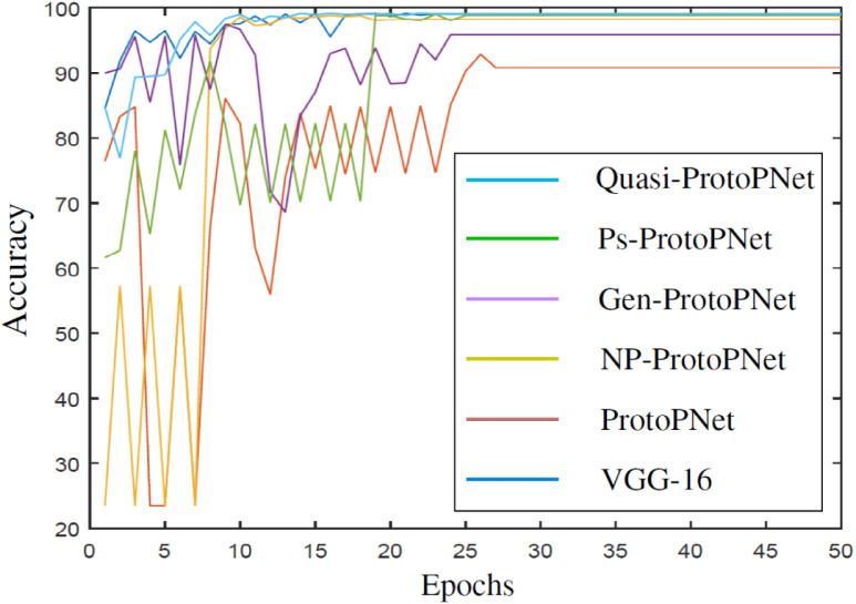
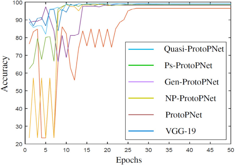
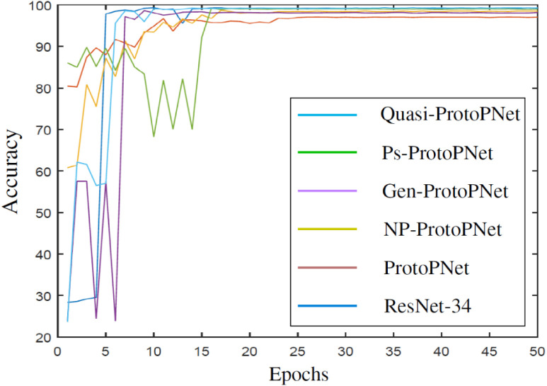
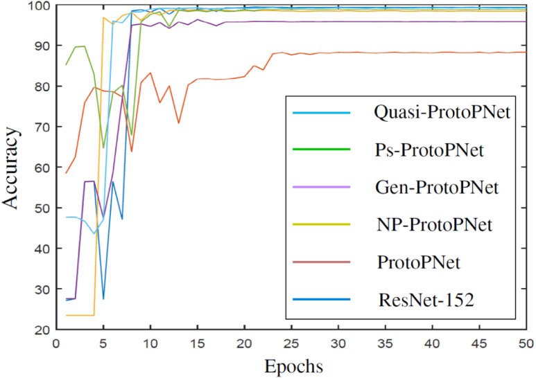
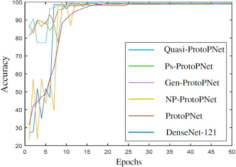
In Fig. 10, Fig. 11, Fig. 12, Fig. 13, Fig. 14, Fig. 15, graphical comparison of the accuracies given by Quasi-ProtoPNet and the other models is provided. Although, the accuracies given the models become stable before $35$ epochs, the models are trained and tested for $100$ epochs over the dataset (Gunraj et al., 2021b), and the graphical comparisons of the accuracies are provided over $50$ epochs.

Fig. 10.

Quasi-ProtoPNet with VGG-16.

Fig. 11.

Quasi-ProtoPNet with VGG-19.

Fig. 12.

Quasi-ProtoPNet with ResNet-34.

Fig. 13.

Quasi-ProtoPNet with ResNet-152.

Fig. 14.

Quasi-ProtoPNet with DenseNet-121.

Fig. 15.

Quasi-ProtoPNet with DenseNet-161.

Fig. 10 provides a comparison of the accuracies given by the models when they are constructed over the convolutional layers of VGG-$16$. Although, it is difficult to see the difference between the accuracies in Fig. 10, Fig. 11, Fig. 12, Fig. 13, Fig. 14, Fig. 15, the difference is clear before the models stabilize.

3.5. The effect of the projection of prototypes

In this section, we prove a theorem similar to Chen et al. (2018, Theorem 2.1). The theorem (Chen et al., 2018 Theorem 2.1) assumes that the negative connections between similarity scores and incorrect classes can be made equal to zero during the training process. As mentioned in Section 1.1, our experiments show that it is hardly possible to make the negative connections zero during the training process. However, we do not need to make this assumption because our model uses only positive reasoning process, and the suspension of the convex optimization of the last layer of our model keeps the connection between similarity scores and incorrect classes zero. Furthermore, (Chen et al., 2018 Theorem 2.1) is proved with the Euclidean distance function, whereas our theorem is neither restricted to the Euclidean distance function nor to its generalized version $d$, but the distance function can be replaced with any positive-valued function that satisfies the triangular inequality and has an appropriate domain. However, we present the theorem with a hemimetric, a distance function more general than the distance function $d$.

Theorem 3.1

Let $f$ be a hemimetric. Suppose $f$ and the distance function $d$ have the same domain, and $f^2$ denotes the square of $f$ . Let $h\circ p_t\circ L$ be a Quasi-ProtoPNet. For a class $k$ , let $a_i^k$ and $b_i^k$ be the values of $i$ th prototype for class $k$ after the projection of $p_i^k$ and before the projection of $p_i^k$ , respectively. Let $x$ be an input image that is correctly classified by Quasi-ProtoPNet before the projection, and $k$ be the correct class label of $x$ . Let ${\mathcal{O}}_i^k$ be the patch of $L\left(x\right)$ closest to $a_i^k$ . Suppose there exists some $\delta$ with $0<\delta <1$ such that:

• 1. for all $k^{\prime }\ne k$ and $i\in \{1,\dots ,m_{k^{\prime }}\}$ , we have $f(a_i^{k^{\prime }},b_i^{k^{\prime }})\le \theta f({\mathcal{O}}_i^{k^{\prime }},b_i^{k^{\prime }})-\sqrt{\epsilon }$ , where $\theta =min(\sqrt{1+\delta }-1,1-\frac{1}{\sqrt{2-\delta }})$ and $\epsilon$ is given by $p_t\left(L\left(x\right)\right)={max}_{\mathcal{P}\in \text{patches}\left(L\left(x\right)\right)}^{}log\left(\frac{f^2(\mathcal{P},p)+1}{f^2(\mathcal{P},p)+\epsilon }\right)$ ;
• 2. for all $i\in \{1,\dots ,m_k\}$ , we have $f(a_i^k,b_i^k)\le (\sqrt{1+\delta }-1)f({\mathcal{O}}_i^k,b_i^k)$ and $f({\mathcal{O}}_i^k,b_i^k)\le \sqrt{1-\delta }$ .

Then after projection,

• 1. the output logit ${\Delta }_k$ (say) for the correct class $k$ can decrease at most by $mlog(1+\delta )(2-\delta )$ , that is, ${\Delta }_k\ge -mlog(1+\delta )(2-\delta )$ ;
• 2. the output logit ${\Delta }_{k^{\prime }}$ (say) for incorrect classes $k^{\prime }$ can increase at most by $mlog(1+\delta )(2-\delta )$ , that is, ${\Delta }_{k^{\prime }}\le mlog(1+\delta )(2-\delta )$ .

Proof

For any class $c$, let $G_c(x,{\left\{p_i^c\right\}}_{i=1}^m)$ be the output logit for input image $x$, where ${\left\{p_i^c\right\}}_{i=1}^m$ denote the prototypes of class $c$. The connection between similarity score and incorrect classes is zero, and the suspension of the convex optimization of the dense layer keep these connections fixed. Therefore,

$$\begin{array}{ccc}\hfill G_c(x,{\left\{p_i^c\right\}}_{i=1}^m)& \hfill =\hfill & \sum _{i=1}^{m}log\left(\frac{f^2({\mathcal{O}}_i^c,p_i^c)+1}{f^2({\mathcal{O}}_i^c,p_i^c)+\epsilon }\right).\hfill \end{array}$$

Let ${\Delta }_c$ be the difference between the output logit of class $c$ after the projection and before the projection of prototypes. Suppose $G_c(x,{\left\{a_i^c\right\}}_{i=1}^m)$ and $G_c(x,{\left\{b_i^c\right\}}_{i=1}^m)$ denote the logits after the projection and before the projection, respectively. Therefore, we have

$$\begin{array}{ccc}{\Delta }_c\hfill & =\hfill & G_c(x,{\left\{a_i^c\right\}}_{i=1}^m)-G_c(x,{\left\{b_i^c\right\}}_{i=1}^m)\hfill \\ \hfill & =\hfill & \sum _{i=1}^{m}log\left(\frac{f^2({\mathcal{O}}_i^c,a_i^c)+1}{f^2({\mathcal{O}}_i^c,b_i^c)+1}\cdot \frac{f^2({\mathcal{O}}_i^c,b_i^c)+\epsilon }{f^2({\mathcal{O}}_i^c,a_i^c)+\epsilon }\right).\hfill \end{array}$$ (8)

Assume,

$$\begin{array}{c}\hfill {\Psi }_i^c=\frac{f^2({\mathcal{O}}_i^c,a_i^c)+1}{f^2({\mathcal{O}}_i^c,b_i^c)+1}\times \frac{f^2({\mathcal{O}}_i^c,b_i^c)+\epsilon }{f^2({\mathcal{O}}_i^c,a_i^c)+\epsilon }.\end{array}$$ (9)

Therefore,

$${\Delta }_c=\sum _{i=1}^{m}log{\Psi }_i^c.$$ (10)

First, to prove 1., that is, to find the lower bound of ${\Delta }_k$, assume $c=k$ in Eqs. (9), (10), where $k$ is the correct class of $x$.

From the inequality given in assumption 2., we have

$$\frac{f^2({\mathcal{O}}_i^k,a_i^k)+1}{f^2({\mathcal{O}}_i^k,b_i^k)+1}\ge \frac{1}{f^2({\mathcal{O}}_i^k,b_i^k)+1}\ge \frac{1}{2-\delta }.$$ (11)

Using the triangular inequality, we have

$$\frac{f^2({\mathcal{O}}_i^k,b_i^k)+\epsilon }{f^2({\mathcal{O}}_i^k,a_i^k)+\epsilon }\ge \frac{f^2({\mathcal{O}}_i^k,b_i^k)+\epsilon }{{(f({\mathcal{O}}_i^k,b_i^k)+f(a_i^k,b_i^k))}^2+\epsilon }.$$ (12)

By assumption 2., we have

$$f(a_i^k,b_i^k)\le (\sqrt{1+\delta }-1)f({\mathcal{O}}_i^k,b_i^k),\text{that is, }$$

$$f(a_i^k,b_i^k)+f({\mathcal{O}}_i^k,b_i^k)\le f({\mathcal{O}}_i^k,b_i^k)\sqrt{1+\delta }.$$ (13)

Square inequality (13) and add $\epsilon$ to the result, we obtain

$$\begin{array}{ccc}\hfill {(f(a_i^k,b_i^k)+f({\mathcal{O}}_i^k,b_i^k))}^2+\epsilon & \hfill \le \hfill & (1+\delta )f^2({\mathcal{O}}_i^k,b_i^k)+\epsilon \hfill \\ \hfill & \hfill \le \hfill & (1+\delta )(f^2({\mathcal{O}}_i^k,b_i^k)+\epsilon ).\hfill \end{array}$$ (14)

On rearranging inequality (14), we have

$$\frac{f^2({\mathcal{O}}_i^k,b_i^k)+\epsilon }{{(f(a_i^k,b_i^k)+f({\mathcal{O}}_i^k,b_i^k))}^2+\epsilon }\ge (1+\delta ).$$ (15)

By inequalities (12), (15), we have

$$\frac{f^2({\mathcal{O}}_i^k,b_i^k)+\epsilon }{f^2({\mathcal{O}}_i^k,a_i^k)+\epsilon }\ge (1+\delta ).$$ (16)

Therefore, by Eqs. (11), (16), we have

$${\Psi }_i^k=\frac{f^2({\mathcal{O}}_i^k,a_i^k)+1}{f^2({\mathcal{O}}_i^k,b_i^k)+1}\times \frac{f^2({\mathcal{O}}_i^k,b_i^k)+\epsilon }{f^2({\mathcal{O}}_i^k,a_i^k)+\epsilon }\ge \frac{1}{(1+\delta )(2-\delta )}.$$ (17)

Hence, by Eqs. (8), (17), we have

$${\Delta }_k\ge \sum _{i=1}^{m}log\left(\frac{1}{(1+\delta )(2-\delta )}\right),\text{ that is, }{\Delta }_k\ge -mlog(1+\delta )(2-\delta ).$$

Second, to prove 2., that is, to find the upper bound of ${\Delta }_{k^{\prime }}$, assume $c=k^{\prime }$ in the above Eqs. (9), (10), where $k^{\prime }$ is the incorrect class of $x$.

By the triangle inequality,

$$\frac{f^2({\mathcal{O}}_i^{k^{\prime }},a_i^{k^{\prime }})+1}{f^2({\mathcal{O}}_i^{k^{\prime }},b_i^{k^{\prime }})+1}\le \frac{{(f({\mathcal{O}}_i^{k^{\prime }},b_i^{k^{\prime }})+f(a_i^{k^{\prime }},b_i^{k^{\prime }}))}^2+1}{f^2({\mathcal{O}}_i^{k^{\prime }},b_i^{k^{\prime }})+1}.$$ (18)

The assumption 1. gives:

$$\begin{array}{ccc}\hfill f(a_i^{k^{\prime }},b_i^{k^{\prime }})& \hfill \le \hfill & (\sqrt{1+\delta }-1)f({\mathcal{O}}_i^{k^{\prime }},b_i^{k^{\prime }})-\sqrt{\epsilon }\hfill \\ \hfill & \hfill \le \hfill & (\sqrt{1+\delta }-1)f({\mathcal{O}}_i^{k^{\prime }},b_i^{k^{\prime }}).\hfill \end{array}$$ (19)

By the inequality (19), we have

$$\begin{array}{ccc}\hfill {(f({\mathcal{O}}_i^{k^{\prime }},b_i^{k^{\prime }})+f(a_i^{k^{\prime }},b_i^{k^{\prime }}))}^2& \hfill \le \hfill & {(f({\mathcal{O}}_i^{k^{\prime }},b_i^{k^{\prime }})+(\sqrt{1+\delta }-1)f({\mathcal{O}}_i^{k^{\prime }},b_i^{k^{\prime }}))}^2\hfill \\ \hfill \\ \hfill & \hfill =\hfill & {\left(\left(\sqrt{1+\delta }\right)f({\mathcal{O}}_i^{k^{\prime }},b_i^{k^{\prime }})\right)}^2=(1+\delta )f^2({\mathcal{O}}_i^{k^{\prime }},b_i^{k^{\prime }}).\hfill \end{array}$$ (20)

The inequality (20) gives:

$$\begin{array}{ccc}\hfill \frac{{(f({\mathcal{O}}_i^{k^{\prime }},b_i^{k^{\prime }})+f(a_i^{k^{\prime }},b_i^{k^{\prime }}))}^2+1}{f^2({\mathcal{O}}_i^{k^{\prime }},b_i^{k^{\prime }})+1}& \hfill \le \hfill & \frac{(1+\delta )f^2({\mathcal{O}}_i^{k^{\prime }},b_i^{k^{\prime }})+1}{f^2({\mathcal{O}}_i^{k^{\prime }},b_i^{k^{\prime }})+1}\hfill \\ \hfill \\ \hfill & \hfill \le \hfill & \frac{(1+\delta )f^2({\mathcal{O}}_i^{k^{\prime }},b_i^{k^{\prime }})+1+\delta }{f^2({\mathcal{O}}_i^{k^{\prime }},b_i^{k^{\prime }})+1}\hfill \\ \hfill & \hfill =\hfill & 1+\delta .\hfill \end{array}$$ (21)

From the inequalities (18), (21), we have

$$\frac{f^2({\mathcal{O}}_i^{k^{\prime }},a_i^{k^{\prime }})+1}{f^2({\mathcal{O}}_i^{k^{\prime }},b_i^{k^{\prime }})+1}\le 1+\delta .$$ (22)

Again, by the triangle inequality, we have

$$f({\mathcal{O}}_i^{k^{\prime }},a_i^{k^{\prime }})\ge f({\mathcal{O}}_i^{k^{\prime }},b_i^{k^{\prime }})-f(a_i^{k^{\prime }},b_i^{k^{\prime }}).$$ (23)

The assumption 1. implies $f({\mathcal{O}}_i^{k^{\prime }},b_i^{k^{\prime }})-f(a_i^{k^{\prime }},b_i^{k^{\prime }})>0$. Therefore, by the inequality (23), we have

$$\begin{array}{ccc}\hfill \frac{f^2({\mathcal{O}}_i^{k^{\prime }},b_i^{k^{\prime }})+\epsilon }{f^2({\mathcal{O}}_i^{k^{\prime }},a_i^{k^{\prime }})+\epsilon }& \hfill \le \hfill & \frac{f^2({\mathcal{O}}_i^{k^{\prime }},b_i^{k^{\prime }})+\epsilon }{{(f({\mathcal{O}}_i^{k^{\prime }},b_i^{k^{\prime }})-f(a_i^{k^{\prime }},b_i^{k^{\prime }}))}^2+\epsilon }\hfill \\ \hfill & \hfill \le \hfill & {\left(\frac{f({\mathcal{O}}_i^{k^{\prime }},b_i^{k^{\prime }})+\sqrt{\epsilon }}{f({\mathcal{O}}_i^{k^{\prime }},b_i^{k^{\prime }})-f(a_i^{k^{\prime }},b_i^{k^{\prime }})}\right)}^2.\hfill \end{array}$$ (24)

Again, by assumption 1., we have

$$f(a_i^{k^{\prime }},b_i^{k^{\prime }})\le \left(1-\frac{1}{\sqrt{2-\delta }}\right)f({\mathcal{O}}_i^{k^{\prime }},b_i^{k^{\prime }})-\sqrt{\epsilon }.$$

On simplifying the above inequality, we obtain

$$\frac{1}{\sqrt{2-\delta }}f({\mathcal{O}}_i^{k^{\prime }},b_i^{k^{\prime }})+\sqrt{\epsilon }\le f({\mathcal{O}}_i^{k^{\prime }},b_i^{k^{\prime }})-f(a_i^{k^{\prime }},b_i^{k^{\prime }}).$$

Therefore,

$$\begin{array}{ccc}\hfill \frac{1}{\sqrt{2-\delta }}f({\mathcal{O}}_i^{k^{\prime }},b_i^{k^{\prime }})+\frac{\sqrt{\epsilon }}{\sqrt{2-\delta }}& \hfill \le \hfill & \frac{1}{\sqrt{2-\delta }}f({\mathcal{O}}_i^{k^{\prime }},b_i^{k^{\prime }})+\sqrt{\epsilon }\hfill \\ \hfill & \hfill \le \hfill & f({\mathcal{O}}_i^{k^{\prime }},b_i^{k^{\prime }})-f(a_i^{k^{\prime }},b_i^{k^{\prime }}).\hfill \end{array}$$ (25)

By the inequality (25), we have

$$\frac{f({\mathcal{O}}_i^{k^{\prime }},b_i^{k^{\prime }})+\sqrt{\epsilon }}{f({\mathcal{O}}_i^{k^{\prime }},b_i^{k^{\prime }})-f(a_i^{k^{\prime }},b_i^{k^{\prime }})}\le \sqrt{2-\delta }.$$ (26)

On combining the inequalities (24), (26), we obtain

$$\frac{f({\mathcal{O}}_i^{k^{\prime }},b_i^{k^{\prime }})+\epsilon }{f({\mathcal{O}}_i^{k^{\prime }},a_i^{k^{\prime }})+\epsilon }\le {\left(\sqrt{2-\delta }\right)}^2=2-\delta .$$ (27)

On combining the inequalities (23), (27), we have

$${\Psi }_i^{k^{\prime }}=\frac{f^2({\mathcal{O}}_i^{k^{\prime }},a_i^{k^{\prime }})+1}{f^2({\mathcal{O}}_i^k,b_i^k)+1}\times \frac{f^2({\mathcal{O}}_i^k,b_i^k)+\epsilon }{f^2({\mathcal{O}}_i^{k^{\prime }},a_i^{k^{\prime }})+\epsilon }\le (1+\delta )(2-\delta ).$$ (28)

Therefore, by Eq. (10), and inequality (28), we have

$$\begin{array}{ccc}\hfill {\Delta }_{k^{\prime }}& \hfill \le \hfill & \sum _{i=1}^{m}log(1+\delta )(2-\delta )\le mlog(1+\delta )(2-\delta ).\hfill \end{array}$$ (29)

Hence, ${\Delta }_{k^{\prime }}\le mlog(1+\delta )(2-\delta )$. □

4. Limitations

As mentioned in Section 1.1, Quasi-ProtoPNet gives better performance than the series of ProtoPNet models when classification is to be made over only a few classes. As the number of classes grows bigger, our model may not give performance better than the performance of ProtoPNet and Ps-ProtoPNet. However, there are many cases similar to the case of CT-scan images as discussed in this paper when we need to classify images over only a few classes. Therefore, our model can be really useful for such situations.

5. Discussion

Quasi-ProtoPNet model suspends the convex optimization of the last layer to keep the connections constant and it uses the objective function that accommodates only the positive reasoning process. Also, the suspension reduced the training time of our model. Quasi-ProtoPNet is closely related to the series of other ProtoPNet models, but strikingly different from them due to its reasoning process for the classifications. Quasi-ProtoPNet uses the positive reasoning process whereas other ProtoPNet models use the negative reasoning process along with the positive reasoning process that leads to decrease in their accuracy, especially when number of classes is small. In particular, our model can be useful during this pandemic when deadly mutants of coronavirus (e.g. omicron variant) are being identified.

6. Conclusions

The use of positive reasoning process along with the use of prototypes with rectangular spatial dimensions and square spatial dimensions helped our model to improve its performance over the series of the other ProtoPNet models. Moreover, as observed in Section 3.2, Quasi-ProtoPNet gives the highest accuracy (99.48%) when DenseNet-$121$ is used as the base model, and the highest accuracy given by Quasi-ProtoPNet is equal to the highest accuracy (99.48%) given by the non-interpretable model DenseNet-$161$.

Declaration of Competing Interest

The authors declare that they have no known competing financial interests or personal relationships that could have appeared to influence the work reported in this paper.

References

- Al-Waisy A.S., Al-Fahdawi S., Mohammed M.A., Abdulkareem K.H., Mostafa S.A., Maashi M.S., et al. COVID-CheXNet: Hybrid deep learning framework for identifying COVID-19 virus in chest X-rays images. Soft Computing. 2020 doi: 10.1007/s00500-020-05424-3. [DOI] [PMC free article] [PubMed] [Google Scholar]
- Al-Waisy A.S., Mohammed M.A., Al-Fahdawi S., Maashi M.S., Garcia-Zapirain B., Abdulkareem K.H., et al. COVID-DeepNet: Hybrid multimodal deep learning system for improving COVID-19 pneumonia detection in chest X-ray images. Computers, Materials & Continua. 2021;67(2):2409–2429. doi: 10.32604/cmc.2021.012955. [DOI] [Google Scholar]
- Bhattacharya S., Reddy Maddikunta P.K., Pham Q.-V., Gadekallu T.R., Krishnan S S.R., Chowdhary C.L., et al. Deep learning and medical image processing for coronavirus (COVID-19) pandemic: A survey. Sustainable Cities and Society. 2021;65 doi: 10.1016/j.scs.2020.102589. [DOI] [PMC free article] [PubMed] [Google Scholar]
- Bien J., Tibshirani R. Prototype selection for interpretable classification. The Annals of Applied Statistics. 2011;5(4):2403–2424. URL: http://www.jstor.org/stable/23069335. [Google Scholar]
- Chaudhary Y., Mehta M., Sharma R., Gupta D., Khanna A., Rodrigues J.J.P.C. 2020 IEEE international conference on e-health networking, application services. 2021. Efficient-CovidNet: Deep learning based COVID-19 detection from chest X-Ray images; pp. 1–6. [DOI] [Google Scholar]
- Chen J.-C., Che Azemin M.Z., Hassan R., Mohd Tamrin M.I., Md Ali M.A. 2020. COVID-19 deep learning prediction model using publicly available radiologist-adjudicated chest X-Ray images as training data: Preliminary findings; pp. 1687–4188. [DOI] [PMC free article] [PubMed] [Google Scholar]
- Chen C., Li O., Barnett A., Su J., Rudin C. 2018. This looks like that: deep learning for interpretable image recognition. CoRR abs/1806.10574, URL: http://arxiv.org/abs/1806.10574. [Google Scholar]
- Clough A., Sharma A., Rani S., Gupta D. Artificial intelligence-based classification of chest X-Ray images into COVID-19 and other infectious diseases. International Journal of Biomedical Imaging. 2020;2020 doi: 10.1155/2020/8889023. [DOI] [PMC free article] [PubMed] [Google Scholar]
- Cohen J.P., Dao L., Roth K., Morrison P., Bengio Y., Abbasi A.F., et al. Predicting COVID-19 Pneumonia severity on chest X-ray with deep learning. Cureus. 2020;12 doi: 10.7759/cureus.9448. [DOI] [PMC free article] [PubMed] [Google Scholar]
- Dansana D., Kumar R., Bhattacharjee A., Hemanth D.J., Gupta D., Khanna A., et al. Early diagnois of COVID-19-affected patients based on X-ray and computed tomography images using deep learning algorithm. Soft Computing. 2020 doi: 10.1007/s00500-020-05275-y. [DOI] [PMC free article] [PubMed] [Google Scholar]
- Erhan D., Bengio Y., Courville A., Vincent P. University of Montreal; 2009. Visualizing higher-layer features of a deep network: Technical Report 1341. URL: https://www.researchgate.net/publication/265022827s_Visualizing_Higher-Layer_Features_of_a_Deep_Network. [Online; Accessed 1 July 2020] [Google Scholar]
- Fu J., Zheng H., Mei T. Proceedings of the IEEE conference on computer vision and pattern recognition. 2017. Look closer to see better: Recurrent attention convolutional neural network for fine-grained image recognition; pp. 4438–4446. URL: https://openaccess.thecvf.com/content_cvpr_2017/html/Fu_Look_Closer_to_CVPR_2017_paper.html. [Online; (Accessed 1 July 2020)] [Google Scholar]
- Ghiasi-Shirazi K. Generalizing the convolution operator in convolutional neural networks. Neural Processing Letters. 2019;50(3):2627–2646. doi: 10.1007/s11063-019-10043-7. [DOI] [Google Scholar]
- Girshick R., Donahue J., Darrell T., Malik J. 2014 IEEE conference on computer vision and pattern recognition. 2014. Rich feature hierarchies for accurate object detection and semantic segmentation; pp. 580–587. [DOI] [Google Scholar]
- Gunraj H., Sabri A., Koff D., Wong A. 2021. COVID-net CT-2: Enhanced deep neural networks for detection of COVID-19 from chest CT images through bigger, more diverse learning. arXiv:arXiv:2101.07433. [DOI] [PMC free article] [PubMed] [Google Scholar]
- Gunraj H., Sabri A., Koff D., Wong A. 2021. COVID-net open source initiative - COVIDx CT-2 dataset. Kaggle, https://www.kaggle.com/hgunraj/covidxct. [Online; (Accessed 7 June 2021)] [Google Scholar]
- Gunraj H., Wang L., Wong A. COVIDNet-CT: A tailored deep convolutional neural network design for detection of COVID-19 cases from chest CT images. Frontiers in Medicine. 2020;7:1025. doi: 10.3389/fmed.2020.608525. URL: https://www.frontiersin.org/article/10.3389/fmed.2020.608525. [DOI] [PMC free article] [PubMed] [Google Scholar]
- He K., Zhang X., Ren S., Sun J. 2016 IEEE conference on computer vision and pattern recognition. 2016. Deep residual learning for image recognition; pp. 770–778. [DOI] [Google Scholar]
- Hinton G.E. Neural networks: tricks of the trade. Springer; 2012. A practical guide to training restricted Boltzmann machines; pp. 599–619. [DOI] [Google Scholar]
- Huang G., Liu Z., Van Der Maaten L., Weinberger K.Q. 2017 IEEE conference on computer vision and pattern recognition. 2017. Densely connected convolutional networks; pp. 2261–2269. [DOI] [Google Scholar]
- Huang S., Xu Z., Tao D., Zhang Y. 2015. Part-stacked CNN for fine-grained visual categorization. CoRR abs/1512.08086, URL: http://arxiv.org/abs/1512.08086. [Google Scholar]
- Jain R., Gupta M., Tanjea S., Jude H.D. Deep learning based detection and analysis of COVID-19 on chest X-ray images. Applied Intelligence: The International Journal of Artificial Intelligence, Neural Networks, and Complex Problem-Solving Technologies. 2020;51:1690–1700. doi: 10.1007/s10489-020-01902-1. [DOI] [PMC free article] [PubMed] [Google Scholar]
- Jain G., Mittal D., Thakur D., Mittal M.K. A deep learning approach to detect Covid-19 coronavirus with X-Ray images. Biocybernetics and Biomedical Engineering. 2020;40:1391–1405. doi: 10.1016/j.bbe.2020.08.008. [DOI] [PMC free article] [PubMed] [Google Scholar]
- Kumar R., Arora R., Bansal V., Sahayasheela V.J., Buckchash H., Imran J., et al. 2020. Accurate prediction of COVID-19 using chest X-Ray images through deep feature learning model with SMOTE and machine learning classifiers. MedRxiv. [DOI] [Google Scholar]
- Lee H., Grosse R., Ranganath R., Ng A.Y. Proceedings of the 26th annual international conference on machine learning. Association for Computing Machinery; New York, USA: 2009. Convolutional deep belief networks for scalable unsupervised learning of hierarchical representations; pp. 609–616. (ICML09). [DOI] [Google Scholar]
- Li O., Liu H., Chen C., Rudin C. 2017. Deep learning for case-based reasoning through prototypes: A neural network that explains its predictions. CoRR abs/1710.04806, URL: http://arxiv.org/abs/1710.04806. [Google Scholar]
- Nalaie K., Ghiasi-Shirazi K., Akbarzadeh-T M.-R. 2017 7th international conference on computer and knowledge engineering. IEEE; Mashhad, Iran: 2017. Efficient implementation of a generalized convolutional neural networks based on weighted euclidean distance; pp. 211–216. [DOI] [Google Scholar]
- Nguyen A., Dosovitskiy A., Yosinski J., Brox T., Clune J. 2016. Synthesizing the preferred inputs for neurons in neural networks via deep generator networks. arXiv:1605.09304. [Google Scholar]
- Ozturk T., Talo M., Yildirim E.A., Baloglu U.B., Yildirim O., Rajendra Acharya U. Automated detection of COVID-19 cases using deep neural networks with X-ray images. Computers in Biology and Medicine. 2020;121 doi: 10.1016/j.compbiomed.2020.103792. [DOI] [PMC free article] [PubMed] [Google Scholar]
- Papernot N., McDaniel P.D. 2018. Deep k-nearest neighbors: Towards confident, interpretable and robust deep learning. CoRR abs/1803.04765, URL: http://arxiv.org/abs/1803.04765. [Google Scholar]
- Priebe C.E., Marchette D.J., DeVinney J., Socolinsky D.A. Classification using class cover catch digraphs. Journal of Classification. 2003;20:003–023. doi: 10.1007/s00357-003-0003-7. [DOI] [Google Scholar]
- Rajaraman S., Sornapudi S., Alderson P.O., Folio L.R., Antani S.K. Analyzing inter-reader variability affecting deep ensemble learning for COVID-19 detection in chest radiographs. PLoS One. 2020;15(11):1–32. doi: 10.1371/journal.pone.0242301. [DOI] [PMC free article] [PubMed] [Google Scholar]
- Reddy G.T., Bhattacharya S., Siva Ramakrishnan S., Chowdhary C.L., Hakak S., Kaluri R., et al. 2020 international conference on emerging trends in information technology and engineering. 2020. An ensemble based machine learning model for diabetic retinopathy classification; pp. 1–6. [DOI] [Google Scholar]
- Ren S., He K., Girshick R., Sun J. In: Advances in neural information processing systems. Cortes C., Lawrence N., Lee D., Sugiyama M., Garnett R., editors. Vol. 28. Curran Associates, Inc.; 2015. Faster R-CNN: Towards real-time object detection with region proposal networks; pp. 91–99. URL: https://proceedings.neurips.cc/paper/2015/file/14bfa6bb14875e45bba028a21ed38046-Paper.pdf. [Google Scholar]
- Richard J., Miller I., Freund J. 9th ed. Pearson; Harlow: 2017. Probability and statistics for engineers. [Google Scholar]
- Salakhutdinov R., Hinton G. In: Proceedings of the eleventh international conference on artificial intelligence and statistics. Meila M., Shen X., editors. vol. 2. PMLR; San Juan, Puerto Rico: 2007. Learning a nonlinear embedding by preserving class neighbourhood structure; pp. 412–419. (Proceedings of machine learning research). URL: https://proceedings.mlr.press/v2/salakhutdinov07a.html. [Google Scholar]
- Simon M., Rodner E. 2015 IEEE international conference on computer vision. 2015. Neural activation constellations: Unsupervised part model discovery with convolutional networks; pp. 1143–1151. [DOI] [Google Scholar]
- Simonyan K., Vedaldi A., Zisserman A. Workshop at international conference on learning representations. Citeseer; 2014. Deep inside convolutional networks: Visualising image classification models and saliency maps; pp. 1–8. URL: https://arxiv.org/abs/1312.6034. [Google Scholar]
- Simonyan K., Zisserman A. 2015. Very deep convolutional networks for large-scale image recognition. CoRR abs/1409.1556, URL: https://arxiv.org/abs/1409.1556. [Google Scholar]
- Singh G., Yow K.-C. An interpretable deep learning model for Covid-19 detection with chest X-Ray images. IEEE Access. 2021;9:85198–85208. doi: 10.1109/ACCESS.2021.3087583. [DOI] [PMC free article] [PubMed] [Google Scholar]
- Singh G., Yow K.-C. Object or background: An interpretable deep learning model for COVID-19 detection from CT-scan images. Diagnostics. 2021;11(9):1732. doi: 10.3390/diagnostics11091732. [DOI] [PMC free article] [PubMed] [Google Scholar]
- Singh G., Yow K.-C. These do not look like those: An interpretable deep learning model for image recognition. IEEE Access. 2021;9:41482–41493. doi: 10.1109/ACCESS.2021.3064838. [DOI] [PMC free article] [PubMed] [Google Scholar]
- Smilkov D., Thorat N., Kim B., Viégas F.B., Wattenberg M. 2017. SmoothGrad: removing noise by adding noise. CoRR abs/1706.03825, URL: http://arxiv.org/abs/1706.03825. [Google Scholar]
- Sundararajan M., Taly A., Yan Q. 2017. Axiomatic attribution for deep networks. CoRR abs/1703.01365, URL: http://arxiv.org/abs/1703.01365. [Google Scholar]
- Uijlings J.R.R., van de Sande K.E.A., Gevers T., Smeulders A.W.M. Selective search for object recognition. International Journal of Computer Vision. 2013;104:154–171. doi: 10.1007/s11263-013-0620-5. [DOI] [Google Scholar]
- Weinberger K.Q., Saul L.K. Distance metric learning for large margin nearest neighbor classification. Journal of Machine Learning Research. 2009;10(9):207–244. URL: http://jmlr.org/papers/v10/weinberger09a.html. [Google Scholar]
- Wexler R. 2017. When a computer program keeps you in jail: How computers are harming criminal justice, new york times. https://www.nytimes.com/2017/06/13/opinion/how-computers-are-harming-criminal-justice.html. [Online; (Accessed 20 January 2021)] [Google Scholar]
- WHO R. 2021. The effects of virus variants on COVID-19 vaccines. https://www.who.int/news-room/feature-stories/detail/the-effects-of-virus-variants-on-covid-19-vaccines. [Online; (Accessed 20 November 2021)] [Google Scholar]
- Wikipedia contributors R. 2021. Accuracy and precision — Wikipedia, the free encyclopedia. https://en.wikipedia.org/w/index.php?title=Accuracy_and_precision&oldid=1054342391. [Online; (Accessed 15 November 2021)] [Google Scholar]
- Wikipedia contributors R. 2021. F-score — Wikipedia, the free encyclopedia. https://en.wikipedia.org/w/index.php?title=F-score&oldid=1054927460. [Online; (Accessed 15 November 2021)] [Google Scholar]
- Wikipedia contributors R. 2021. Precision and recall — Wikipedia, the free encyclopedia. https://en.wikipedia.org/w/index.php?title=Precision_and_recall&oldid=1050491609. [Online; (Accessed 15 November 2021)] [Google Scholar]
- Wu C., Tabak E.G. 2017. Prototypal analysis and prototypal regression. arXiv:1701.08916. [Google Scholar]
- Xiao T., Xu Y., Yang K., Zhang J., Peng Y., Zhang Z. 2015 IEEE Conference on computer vision and pattern recognition, vol. 10, no. 9. 2015. The application of two-level attention models in deep convolutional neural network for fine-grained image classification; pp. 842–850. URL: http://arxiv.org/abs/1411.6447. [Google Scholar]
- Yan C., Gong B., Wei Y., Gao Y. Deep multi-view enhancement hashing for image retrieval. IEEE Transactions on Pattern Analysis and Machine Intelligence. 2021;43(4):1445–1451. doi: 10.1109/TPAMI.2020.2975798. [DOI] [PubMed] [Google Scholar]
- Yan C., Hao Y., Li L., Yin J., Liu A., Mao Z., et al. Task-adaptive attention for image captioning. IEEE Transactions on Circuits and Systems for Video Technology. 2022;32(1):43–51. doi: 10.1109/TCSVT.2021.3067449. [DOI] [Google Scholar]
- Yan C., Li Z., Zhang Y., Liu Y., Ji X., Zhang Y. Depth image denoising using nuclear norm and learning graph model. ACM Transactions on Multimedia Computing Communications and Applications. 2020;16(4):1–17. doi: 10.1145/3404374. [DOI] [Google Scholar]
- Yan C., Meng L., Li L., Zhang J., Yin J., Jhang J., et al. Age-invariant face recognition by multi-feature fusion and decomposition with self-attention. ACM Transactions on Multimedia Computing, Communications and Applications. 2022;18(29):1–18. doi: 10.1145/3472810. [DOI] [Google Scholar]
- Yan C., Teng T., Liu Y., Zhang Y., Wang H., Ji X. Precise no-reference image quality evaluation based on distortion identification. ACM Transactions on Multimedia Computing Communications and Applications. 2021;17(3s):1–21. doi: 10.1145/3468872. [DOI] [Google Scholar]
- Yosinski J., Clune J., Nguyen A.M., Fuchs T.J., Lipson H. 2015. Understanding neural networks through deep visualization. CoRR abs/1506.06579, URL: http://arxiv.org/abs/1506.06579. [Google Scholar]
- Zebin T., Rezvy S.R. COVID-19 detection and disease progression visualization: Deep learning on chest X-rays for classification and coarse localization. Applied Intelligence: The International Journal of Artificial Intelligence, Neural Networks, and Complex Problem-Solving Technologies. 2020;50:1–12. doi: 10.1007/s10489-020-01867-1. [DOI] [PMC free article] [PubMed] [Google Scholar]
- Zeiler M.D., Fergus R. Computer vision. Springer International Publishing; Cham: 2014. Visualizing and understanding convolutional networks; pp. 818–833. [DOI] [Google Scholar]
- Zhang N., Donahue J., Girshick R., Darrell T. Computer vision. Springer International Publishing; Cham: 2014. Part-based R-CNNs for fine-grained category detection; pp. 834–849. [DOI] [Google Scholar]
- Zheng H., Fu J., Mei T., Luo J. 2017 IEEE international conference on computer vision. IEEE; Venice, Italy: 2017. Learning multi-attention convolutional neural network for fine-grained image recognition; pp. 5219–5227. [DOI] [Google Scholar]
- Zhou B., Khosla A., Lapedriza A., Oliva A., Torralba A. 2016 IEEE conference on computer vision and pattern recognition. IEEE; Las Vegas, USA: 2016. Learning deep features for discriminative localization; pp. 2921–2929. [DOI] [Google Scholar]
- Zhou B., Sun Y., Bau D., Torralba A. Proceedings of the European conference on computer vision. 2018. Interpretable basis decomposition for visual explanation; pp. 119–134. URL: https://openaccess.thecvf.com/content_ECCV_2018/html/Antonio_Torralba_Interpretable_Basis_Decomposition_ECCV_2018_paper.html. [Google Scholar]