Climate extremes, variability, and trade shape biogeographical patterns of alien species

Abstract

Understanding how alien species assemble is crucial for predicting changes to community structure caused by biological invasions and for directing management strategies for alien species, but patterns and drivers of alien species assemblages remain poorly understood relative to native species. Climate has been suggested as a crucial filter of invasion-driven homogenization of biodiversity. However, it remains unclear which climatic factors drive the assemblage of alien species. Here, we compiled global data at both grid scale (2,653 native and 2,806 current grids with a resolution of 2° × 2°) and administrative scale (271 native and 297 current nations and sub-nations) on the distributions of 361 alien amphibians and reptiles (herpetofauna), the most threatened vertebrate group on the planet. We found that geographical distance, a proxy for natural dispersal barriers, was the dominant variable contributing to alien herpetofaunal assemblage in native ranges. In contrast, climatic factors explained more unique variation in alien herpetofaunal assemblage after than before invasions. This pattern was driven by extremely high temperatures and precipitation seasonality, 2 hallmarks of global climate change, and bilateral trade which can account for the alien assemblage after invasions. Our results indicated that human-assisted species introductions combined with climate change may accelerate the reorganization of global species distributions.

Long-distance human-aided introductions have allowed alien species to overcome geographical dispersal barriers and limitations from biotic interaction in their native ranges (Capinha et al. 2015). This has resulted in a modification of classic biogeography and a modern-day homogenization of biodiversity (Rahel 2000; Olden et al. 2008; Villeger et al. 2011; Bernardo-Madrid et al. 2019 ). Understanding which factors influence the assemblages of invasive species is a particularly urgent scientific question facing the world today with the potential for the answer to direct management and policy (Pyšek et al. 2010; Redding et al. 2019). In addition to human-assisted dispersal factors, such as bilateral trade, climate has been documented as a crucial factor predicting global assemblage patterns of alien species (Capinha et al. 2015). Several climatic factors, including optimal climatic conditions (Hughes et al. 1996), the magnitude of climatic variability (Stevens 1989), and extreme temperatures (Gaston and Chown 1999), have been proposed to dictate species distributions either directly, by exceeding critical thresholds of organisms (i.e., critical thermal minima and maxima), or indirectly, by determining the availability of key resources, such as water and food (Hurlbert and Haskell 2003). In addition, climatic extremes and variability tend to be more sensitive than climatic averages to climate change (Easterling et al. 2000; Palmer and Ralsanen 2002). Consequently, understanding the degree to which climatic factors account for species composition before and after invasion is not only crucial for understanding the role of climate in invasion success, but also for providing insights into range shifts of both native and invasive species in an era of climate change (Blois et al. 2013a). Although previous studies provided valuable insights into the relative importance of climate and dispersal-related factors in shaping the distribution of alien species before and after invasions (Qian and Ricklefs 2006; Capinha et al. 2015), these studies did not thoroughly explore which components of climate were most important.

Amphibians and reptiles provide an ideal opportunity to address this knowledge gap on role of specific climatic factors in the redistribution of alien species because both temperature and precipitation are considered to have marked effects on the distributions, range sizes, and species compositional patterns of ectotherms (Araújo et al. 2008). Second, there are relatively accurate distributional records of alien amphibians and reptiles in their native and invaded ranges (Kraus 2009; Li et al. 2016a; Capinha et al. 2017; Liu et al. 2019), allowing us to precisely quantify their occupied climatic niches before and after invasions. Finally, herpetofauna is arguably the most threatened of terrestrial vertebrates on the planet (Hoffmann et al. 2010), and their declines have been clearly linked to human-assisted introductions of herpetofaunal species and the deadly pathogens they can carry (Fisher et al. 2012). Here, based on the distributional records of 361 alien amphibians and reptiles in their native and invaded ranges (Supplementary Table S1), we explore the unique contributions of different climatic factors to their global assemblage patterns before and after invasions after controlling for natural dispersal limitations (geographical distance) and anthropogenic dispersal-related factors (bilateral trade). We build on Capinha et al.’s (2015) seminal work on the biogeographical patterns of alien gastropods by adapting and advancing their analyses which involve hierarchical cluster analyses, ordination techniques, and generalized dissimilarity modeling (GDM), which were approaches widely used in biogeographical studies (e.g., Ferrier et al. 2007; Kreft and Jetz 2010; Blois et al. 2013a; Holt et al. 2013; Supplementary Figure S1).

We hypothesize that assemblages of alien herpetofauna were predominantly associated with dispersal limitations in their native ranges. That is, we postulate that, historically, there were suitable climatic conditions for many herpetofaunal species in other parts of the world but they could not successfully disperse to them. With the vast increase in the movement of people and products, we hypothesize that long-distance dispersal is less of a limitation now than it was historically and thus, the distribution of alien herpetofauna is more a function of appropriate climatic conditions than dispersal barriers in their current range. Given the narrow thermal breadths of many herpetofaunal species and the reliance of most amphibians on ample moisture (Li et al. 2013; Rohr et al. 2018), we hypothesize that temperature extremes and precipitation variability might be the predominant climatic factors associated with the modern-day assemblage of alien herpetofauna.

Materials and Methods

Datasets

Species distribution datasets

To capture all species’ distribution and occupied climatic niches, we followed previous studies by focusing on alien species with exact native and introduced range information, and conducted analyses comparing the native and current assemblages before and after their invasions (Capinha et al. 2015). The alien species list is based on a widely used database on global amphibian and reptile introductions compiled by Kraus (2009) and recent updates for their establishment during the last decade (Li et al. 2016a; Capinha et al. 2017; Liu et al. 2019; Liu et al. 2020; Supplementary Table S1). Following the criterion of the Kraus (2009) database, we excluded species re-introduced into a species’ native range, released within their native ranges, experimentally introduced into small islets, and that represented questionable introductions without robust evidence. Furthermore, we only used those successful invaders that have established feral populations in non-native ranges (Blackburn et al. 2011). The species native range is determined based on native-range maps of the International Union for Conservation of Nature (IUCN; https://www.iucnredlist.org/resources/spatial-data-download) and validated using other databases, references such as the recent distributional update of global reptiles (Roll et al. 2017), and regional field guides (Supplementary Table S1). The Kraus (2009) and Capinha et al. (2017) databases provided the species list and the national or sub-national information where the species established. However, it makes no sense to use the average climates calculated across coarse range maps, which does not provide any information on the conditions experienced by species living only in some specific areas of a country. Therefore, we collected occurrence data for each alien amphibian and reptile species in both their native and invaded ranges from various databases and an intensive review of published references (Supplementary Table S1). We removed duplicated records among data sources and species whose native ranges are unknown or without precise geographical location data (based on the expert opinion of Fred Kraus).

Analyses of species composition dissimilarity can be influenced by a study’s scale (e.g., grid level, landscape level, or administrative level) (Steinbauer et al. 2012). Therefore, to test whether our results were sensitive to spatial scale, we conducted our analyses at both grid and administrative level, respectively. In the main manuscript, we present analyses at the grid level because it can control the effect of area on results. We conducted the grid-level analyses at a resolution of 2° × 2°, a resolution frequently used in global biogeography studies (e.g., Holt et al. 2013). We re-conducted all analyses at the administrative level at which the trade data are available (Capinha et al. 2015; Murray et al. 2015; Dawson et al. 2017).

In sum, we used 361 species including 108 amphibians and 253 reptiles. These species occupied a total of 368,766 native and 414,374 current occurrences assigned to a total of 2,653 native and 2,806 current 2° ×  2° grids belonging to 271 native and 297 current (sub)nations based on global administrative area designations (www.gadm.org). We checked species synonyms from different taxonomic authorities for amphibians, squamates, crocodilians, serpents, and turtles (Supplementary Text S1).

Climatic average, variation, and extremes

We used a total of 8 climatic variables to describe temperature and precipitation averages, variation, and extremes, which were extracted based on the occurrence data for native and current ranges from the WorldClim database (version 1.4) at a resolution of 10 arc-minute, and averaged each of 8 variables over each country (Capinha et al. 2015). This database was based on meteorological average monthly climate data recorded from 1950 to 2000 (Hijmans et al. 2005). These 8 bioclimatic variables represent annual trends (e.g., mean annual temperature, annual precipitation), seasonality (e.g., annual range in temperature and precipitation), and extreme or limiting climatic factors (e.g., maximum and minimum temperature of the coldest and warmest month, and precipitation of the wettest and driest month). Climate average refers to the average annual temperature (T_av, Bio1) and average annual precipitation (P_av, Bio12) across all 10-min grid cells encompassed by all species in that region. Climate seasonality refers to the temperature (T_sea, Bio4, standard deviation) or precipitation seasonality (P_sea, Bio15, coefficient of variation) calculated as the average value across occupied grid cells by all species in each region (Pither 2003). In the climate literature, climate extreme usually refers to extreme weather and climate events, such as heat waves, cold waves, droughts, and storms, exceeding climate thresholds on a particular occasion (Easterling et al. 2000). In the macroecological and biogeographical literature, “climate extreme” is usually classified as the maximum temperature, minimum temperature, maximum precipitation, and minimum precipitation at any grid cell within the geographic range of a focal species based on averaging monthly data from public climate database (Pither 2003; Li et al. 2016b). Here, we followed this latter classification of extremes. More specifically, as there are usually multiple species in each grid/nation or sub-nation, we first extracted the highest or the lowest value of the maximum or minimum temperature of the hottest (T_max, Bio5) or the coldest month (T_min, Bio6) and the highest or the lowest value of average precipitation of the wettest (P_max, Bio13) or the driest month (P_min, Bio14) encountered by each species in each grid/nation or sub-nation. We then averaged the extracted highest or lowest T_max, T_min, P_max, and P_min values per species in the same grid/nation or sub-nation to represent the average climate extreme of the grid/nation or sub-nation. These 8 climatic variables were selected because they reflect climate average, variability, and extremes that can be important to species distributions (Janzen 1967; Li et al. 2016b). Moreover, pairwise Pearson rank correlation analyses (at which scale the cluster, ordination, and GDM analyses were performed) revealed that the correlation coefficients of these 8 climatic predictors were all <0.75 (Supplementary Table S2), a commonly used cutoff for evaluating climatic collinearity in modeling climate effects on species distributions (Capinha et al. 2015). Thus, these 8 variables were not highly collinear.

Although previous studies suggested that amphibians and reptiles usually have different climatic requirements, as reptiles are particularly rich in hot and dry climates, whereas amphibians are strongly associated with humid climates (Powney et al. 2010), we did not find significant differences in the climatic variables between distributional ranges occupied by amphibians and reptiles (Supplementary Figure S2). Although certain microhabitats might vary among taxa, our results were consistent with previous macroecological studies showing that climatic variables tend to be similar for amphibians and reptiles, reflecting their general physiological requirements for water and energy (Araújo and Pearson 2005). Consequently, as the sample size of amphibians (108 species) is much smaller than reptiles (253 species, Supplementary Table S1), we combined the 2 taxa together to provide a more robust analysis based on a larger sample size.

Natural dispersal and trade data

We used geographical distance calculated based on the geographical coordinates of centroids of each pair of grids (nations or sub-nations at the administrative scale) as a comprehensive proxy of the natural dispersal barriers of species (Blois et al. 2013b; Capinha et al. 2015). It has been widely reported that range expansions of alien species can be associated with human-assisted dispersal factors, such as trade (Essl et al. 2015; Dyer et al. 2016). We, therefore, used average bilateral trade data for the sub-samples of current ranges (2,651 grids across 183 countries, in US dollars across the years of 1962–2010) from the UN trade database (https://comtrade.un.org) to test for the effect of bilateral trade on the species assemblage pattern after invasions (Essl et al. 2015). For countries (e.g., USA, Canada, Australia, and China) that are subdivided into multiple areas, we re-calculated the species compositional dissimilarity, and different climatic and dispersal-related variables for each country as a whole. To calculate bilateral trade, we first calculated all traded commodities (imports and exports) of country i with j, and then divided by the total trade of country i with the world (Capinha et al. 2015). For the grid-level analysis, those grids in the same country were assigned the same trade values.

Delineation of alien species assemblages

Species compositional dissimilarity

We quantified pairwise compositional dissimilarity among grids/nations or sub-nations using the turnover component of the Baselga’s dissimilarity β_sim index (Baselga 2010), which is widely used as a standard index in biogeography and macroecology studies because it robust to differences in species richness among countries (Kreft and Jetz 2010), and to differences in sample size between grids/nations or sub-nations being compared (Barwell et al. 2015). The β_sim was expressed as follows:

$$\mathrm{\beta }\mathrm{sim}\mathrm{ }=1-\frac{a}{\min \left(b,c\right)+a}$$

(1) where a refers to the number of shared species between 2 grids (nations or sub-nations) i and j, b refers to the number of species found in grid (nation or sub-nation) i but not grid (nation or sub-nation) j, and c is the number of species found in grid (nation or sub-nation) j but not grid (nation or sub-nation) i. β_sim varies from 0 to 1, with low β_sim values indicating that grid (nation or sub-nation) i and j share many similar taxa (i.e., 0, complete similarity) and a high β_sim values indicating that grid (nation or sub-nation) i and j share a small number of similar taxa (i.e., 1, complete dissimilarity). The application of the β_sim index resulted in 3,517,878 and 3,935,415 pairwise distance values at the grid scale, and 36,585 and 43,956 pairwise distance at the administrative scale for native and current ranges, respectively. The β_sim index was calculated using the betapart package (Baselga and Orme 2012) in R (Core T 2016).

Hierarchical cluster and ordination analyses

Both hierarchical clustering and ordination techniques were used to calculate and visualize the spatial patterns of compositional similarity based on the β_sim index. We conducted cluster analyses using an unweighted pair-group method based on arithmetic averages (UPGMA), which is frequently used in large-scale biogeographical studies (Kreft and Jetz 2010). UPGMA is a hierarchical clustering technique that classifies different grids/nations or sub-nations with similar species composition into clusters within a dendrogram. We also analyzed the species compositional similarity using 6 other clustering techniques including the weighted pair-group method based on arithmetic averages (McQuitty’s method), Ward’s minimum variance, Median, Centroid, Single, and Complete method (Kreft and Jetz 2010) (descriptions on each cluster method are shown in Supplementary Table S3). We evaluated the accuracy of different cluster methods in converting the dissimilarity matrices into dendrograms using cophenetic correlation coefficients, which measure the agreement between cluster assignments and the original compositional dissimilarity matrix (Legendre and Legendre 2012). We found that UPGMA method had higher cophenetic correlation coefficient, indicating that it performed better than other methods to quantify pairwise dissimilarity for both native and current ranges (Supplementary Table S4). Based on the UPGMA hierarchical dendrograms, we determined the optimal number of biogeographical regions by applying the Kelley–Gardner–Sutcliffe (KGS) penalty function in the maptree package. KGS is an objective method widely used in biogeographical research to determine the number of distinct clusters. For each level of the hierarchical tree, the KGS penalty is calculated as the average distance between nodes within each cluster plus the number of clusters at the level (Kelley et al. 1996). The KGS penalty maximizes differences between clusters and the cohesiveness within clusters and the level of the tree with the minimum value corresponds to the optimal number of clusters (a detailed process of the method is given in Supplementary Figure S3) (Kelley et al. 1996).

To validate the results of the hierarchical clustering analyses, we also analyzed the data using nonmetric multidimensional scaling (NMDS), which is considered the most robust ordination technique for generating low-dimensional projections by arranging range assemblages based on taxonomic composition (Legendre and Legendre 2012). It is especially useful for visualizing the inter-relationships among different grids/nations or sub-nations according to their taxonomic compositional similarity rather than forcing them into discrete groups (i.e., clusters). Additionally, the generated plot can display ranges that are close to one another in ordination space. NMDS represents the original position of data in multidimensional space as accurately as possible using a reduced number of dimensions that can be plotted and visualized (like principal component analysis). The stress value was used to assess the agreement between the original distances and distances in the reduced ordination space of the NMDS (Legendre and Legendre 2012). Stress value is a goodness-of-fit statistic representing the sum of the squared differences between distances in the reduced dimensional space compared with the complete multidimensional space. It ranges from 0 to 1, with smaller values indicating less of a difference and thus a better fit (Legendre and Legendre 2012). We performed the cluster analysis using hclust function and NMDS analyses using monoMDS function in vegan package (Oksanen et al. 2013).

Predictors of alien species assemblages in native and current ranges

We applied GDM (Ferrier et al. 2007) to investigate the drivers of assemblage patterns of alien species in native and current ranges. GDM has been widely used to identify the independent contributions of different factors explaining species compositional dissimilarity (e.g., Blois et al. 2013a; Fitzpatrick et al. 2013; Capinha et al. 2015). Compared with traditional matrix regression approaches, GDM can accommodate nonlinearities of ecological predictors with observed compositional dissimilarity (i.e., β_sim measure) (Ferrier et al. 2007). GDM uses maximum-likelihood estimation and flexible I-splines to explore the relationship between environmental/geographical distance and species compositional dissimilarity (Ferrier et al. 2007). For the administrative-level analysis, to account for the potential influence of country size in representing centroid-based distance, we set weights for each nations or sub-nations according to their ranking in the size distribution. This method is regarded as more robust than weights proportional to country area, which can result in overweighting small island countries. For the grid-level analysis, we set equal weights to each grid. We used the default 3 I-splines basis functions per predictor variable. These 3 coefficients of the I-splines provide the final transformation function representing the best-supported relationship between pairwise distances of predictor variables and observed species compositional dissimilarity (Fitzpatrick et al. 2013). Spatial autocorrelation was accounted for by including the geographical distance between pairs of grids/nations or sub-nations as a predictor variable (Ferrier et al. 2007). Disentangling the relative influence of climatic factors, geographical distance, and human dispersal is challenging as different climatic components may be correlated, and climate might also co-vary with dispersal factors. To achieve this, we followed previous studies using the total height of the transformation function curve, which serves as the relative importance of each variable to species compositional change holding all other variables constant (e.g., “partial ecological distance”), and the shape of the curve reflects the rate of species compositional change along the gradient of the independent variable (Ferrier et al. 2007; Fitzpatrick et al. 2013). The significance of each predictor was tested using Monte Carlo permutation procedures as implemented in the gdm.varImp function (Ferrier et al. 2007). The permutation process was implemented by first calculating the difference in deviance between the models with and without the predictor. Then, this observed deviance difference was compared with a null distribution of deviance differences obtained by fitting the 2 models using random permutations of the order of sites in the compositional dissimilarity matrix. A predictor was considered as nonsignificant if no significant difference was found in deviance between the 2 models (Ferrier et al. 2007; Fitzpatrick et al. 2013; Capinha et al. 2015). We performed 1,000 permutations until all nonsignificant variables were removed. Permutation analyses can test the significance of predictor variables, but cannot quantify parameter uncertainty through confidence interval estimations. In GDM, an estimate of parameter uncertainty, or the variance in fitted I-splines of each predictor, was achieved by a bootstrapping approach using the plotUncertainty function in the gdm package (Shryock et al. 2015). However, evaluation of the uncertainty of overall model fit is unfortunately not available for GDM yet. Consequently, we used the multifaceted biodiversity modelling (MBM) approach based on Gaussian processes to generate the 95% confidence intervals of the overall model fit and qualitatively compared it to the model fit with GDM (Talluto et al. 2018). We then evaluated model fits for MBM and GDM using a root mean square prediction error (RMSE) test with smaller values indicating better performance (Talluto et al. 2018). The MBM analyses were conducted using the mbm package (Talluto et al. 2018) in R. MBM analyses showed similar trends with GDM for changes in species compositional dissimilarity with environmental distance (Supplementary Figure S4). RMSE values for both the GDM and MBM models were very small (0.051–0.070), suggesting a good fit to the data (Supplementary Table S5).

To quantify the unique explained deviances of climatic predictors (D_clim), dispersal predictors (D_dis) and their shared deviances (D_shared) to species compositional dissimilarity, we fit 3 GDMs: (1) only climatic variables; (2) only dispersal predictors including geographical distances in combination with bilateral trade variables; and (3) full models containing all predictors (Blois et al. 2013a; Fitzpatrick et al., 2013; Capinha et al. 2015). D_clim was calculated as the deviance explained by all predictors minus the deviance explained by the model with only dispersal predictors, D_dis as the deviance explained by all predictors minus the deviance explained by the model with only climate, and D_shared as 1—D_clim—D_dis. The relationship between environmental or geographical predictors and compositional dissimilarity is achieved by reformulating traditional matrix regression as a generalized linear model in terms of a link function in inverse form (Ferrier et al. 2007):

$$\mu =\text{ 1 }–e^{-\eta }$$ (2)

where μ is the predicted response variable (i.e., species compositional dissimilarity among sites here), and η is the environmental or geographical distances. To account for the nonlinearity of the rate of species compositional dissimilarity along environmental or geographical gradients, η is then formulated as:

$$\eta =\mathrm{\alpha }+\sum _{p=1}^n\left|f_p\left(x_{pi}\right)-f_p\left(x_{pj}\right)\right|$$ (3)

where n is environmental or geographical variables (x₁ to x_n) from gird/region i to j, f_p (x_p) is the fitting function between predicted and observed compositional dissimilarity as a linear combination of I-spline basis functions:

$$f_p\left(x_p\right)=\sum _{k=1}^{m_p}{a}_{pk}{I}_{pk}\left(x_p\right)$$ (4)

where a_pk (≥0) is a constraint, m_p is the number of I-spline employed, and I_pk is the kth I-spline for variable x_p and a_pk is the fitted coefficient for I_pk.

Sensitivity analyses for data uncertainties

A potential issue in exploring the importance of extreme high temperatures and precipitation seasonality was that our results may be dependent on differences in species introduction opportunities to high versus low-temperature extremes or precipitation seasonality. Although there was a higher proportion of pole-wards (i.e., higher absolute latitude, 65.4%) than equator-wards introductions (i.e., lower absolute latitude, 34.6%) of herpetofaunal species, which was coincident with previous findings on introduction directions of alien mammals, birds, and plants (Guo et al. 2012), we did not detect significant differences in high temperatures (Kruskal–Wallis test: χ² = 2.95, d.f.  = 1, P = 0.204) or precipitation seasonality (χ² = 2.46, d.f.  = 1, P = 0.216) of occupied grids between pole-ward and equator-ward introduction events. This demonstrated that our results were not an artifact of differences in species introduction opportunities along this latitudinal gradient.

Results

Alien species assemblages in native and current ranges

The 361 alien amphibians and reptiles have established populations worldwide (mean ± SE of alien richness: 0.97 ± 0.045 across grids) after 3,516 introduction events in 297 regions (mean ± SE: 12 ± 2.61). There are 17.8% of regions with >50% amphibians and reptiles considered alien species (Supplementary Figure S5). The Atlantic and (sub)tropical Pacific Islands, Florida, and western states of the USA, such as California, western Europe, and southeastern Asia represent hotpots of alien herpetofauna incursions (Supplementary Figure S5). These invasions have resulted in an increase of compositional similarity of the alien herpetofauna in current ranges relative to their native ranges (2-tailed Wilcoxon signed-rank test, Z = −19.80, P < 0.001).

These increases in species compositional similarity have further simplified the global biogeography of alien herpetofauna with significant decreases in the number of assemblages along different levels of UPGMA cluster depths (grid level: native ranges, 27.56 ± 3.79, current ranges, 15.86 ± 3.62, Z = −6.03, P  < 0.001; administrative level: native ranges, 22.18 ± 1.24, current ranges, 14.32 ± 1.37, Z = −6.17, P < 0.001, Supplementary Figure S6). According to the KGS penalty function that aims to objectively identify the optimal number of clusters (Supplementary Figure S7), we found that the assemblages have been simplified from 10 distinct groups in native range to only 4 distinct arrangements in their current range (Figure 1). The native assemblages were generally consistent with the classic zoogeographical classifications, such as Nearctic, Neotropics, Afrotropic, Indo-Mala, Palearctic, and Australia with some Caribbean countries as unique zones (Figure 1). However, after invasions, some distant or isolated islands were no longer distant regions, and some areas were clustered into similar groupings, such as Atlantic islets, Florida U.S., Madagascar, Asia, Australia, and the America (Figure 1). The results of NMDS analyses were highly concordant with the cluster analyses, showing a change from greater dispersion in native ranges to increased similarity among current regions after invasions (Supplementary Figure S8). The stress values both for native distributions and for current distributions were relatively low (0.011 and 0.021, respectively), supporting a good projection of the species compositional dissimilarity matrix into the 2-dimensional ordination space.

Figure 1.

Dendrograms and global maps of compositional similarities for 361 alien amphibians and reptiles at a grid level with a resolution of 2° × 2° for native ranges (A, n = 2,653) and current ranges (B, n = 2,806). Colors represent main groups from the cluster analyses using a UPGMA approach based on the β_sim index. The number of assemblage groups is determined based on the KGS penalty function (Supplementary Figure S7). Caribbean islands included in this study are magnified in the inset.

We obtained similar species assemblage patterns when we excluded American bullfrog (Lithobates catesbeianus = Rana catesbeiana), blind snake Ramphotyphlops braminus, and slider turtle Trachemys scripta (Supplementary Figure S9), which we hypothesized might have significant effects on the biogeographical patterns because of their more widespread introductions than other species. We also obtained similar patterns for remaining regions (i.e., 6 main groups for native ranges and 4 groups for current ranges) after excluding the Atlantic islands where considerable homogenization occurred (Supplementary Figure S10).

Important predictors of alien species assemblages

Overall, the compositional similarity significantly decreased with increasing geographical distance in both native ranges (Spearman correlation coefficient r = −0.427, P < 0.001) and current ranges after invasions (r = −0.365, P < 0.001). However, highly similar species compositions occurred more frequently with increasing geographical distance in current ranges (Supplementary Figure S11). Monte Carlo permutation analyses based on GDMs revealed that geographical distance, precipitation seasonality, and high-temperature extremes were significantly (P < 0.001) correlated with compositional dissimilarity both of native and current ranges. However, the unique variance explained by climate and geographical distance changed greatly after invasions (Figure 2). In native ranges, the unique deviance of geographical distance and climate in explaining compositional dissimilarity was 46.2% and 18.4%, respectively (Figure 2). After invasions, the unique deviance explained by geographical distance decreased to 25.4%, whereas climate explained 35.8% unique deviances of species compositional dissimilarity. When we conducted analyses using subsamples controlling for available bilateral trade data, we obtained a similar result—the unique deviance explained by geographical distance decreased, whereas bilateral trade and climate explained more unique deviances after invasions (Figure 2). When we included bilateral trade in the analysis of native ranges, we found that it was not a significant variable (P = 0.60) in explaining native assemblages of alien species, and it explained much less unique deviance (9.2%) of species compositional dissimilarity in native ranges than current ranges (20.4%) (Figure 2).

Figure 2.

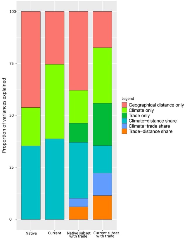
Proportion of unique and shared deviance by climatic and dispersal factors (geographical distance and bilateral trade) for species compositional dissimilarity of 361 alien amphibians and reptiles at a grid level with a resolution of 2° × 2° for native ranges (n = 2,653), current ranges (n = 2,806), and sub-samples of native (n = 2,473) and current ranges (n = 2,651) where bilateral trade data are available.

GDM-fitted I-splines further supported that geographical distance was a dominant predictor with a high relative importance in explaining species compositional dissimilarity in native ranges (Figure 3A-1). In contrast, in current ranges, the relative importance values of climatic factors in explaining species compositional dissimilarity remarkably increased especially for the high-temperature extremes (native: 1.02, current: 2.53, Figure 3A-2 and 3B-2), followed by precipitation seasonality (native: 1.04, current: 1.27, Figure 3A-3 and 3B-3). These 2 climatic variables were also the only 2 significant (P  < 0.001) and most important climatic predictors of species compositional dissimilarity (Figure 3A-2, 3, 3B-2, 3, 3C-2 and 3). The nonlinear shapes of the GDM curves showed an increasing rate of species compositional change with increasing geographical distance (Figure 3A-1, 3B-1 and 3C-1), high-temperature extremes (Figure 3A-2, 3B-2 and 3C-2), precipitation seasonality (Figure 3A-3, 3B-3 and 3C-3), and bilateral trade (Figure 3C-4), but the species composition tended to be stable when geographical distance and high temperatures reached a threshold (Figure 3A-1,2, 3B-1,2 and 3C-1,2). The performance of each predictor variable was stable according to the 95% confidence bands generated by 100 bootstrapping tests (Figure 3).

Figure 3.

GDM-fitted I-splines for significant variables associated with species compositional similarity for alien amphibians and reptiles at a grid level with a resolution of 2° × 2° for native ranges (A, n = 2,653), current ranges (B, n = 2,806), and sub-samples of current ranges where bilateral trade data are available (C, n = 2,651). The maximum height reached by each curve indicates the relative importance of each predictor variable quantified by summing the coefficients of the I-splines from GDM (e.g., “partial ecological distance” holding all other variables constant). The shape of each function provides an indication of how the rate of compositional similarity varies along the environmental gradient. The gray color shows the confidence bands permutating 100 times of bootstrapping using 70% subsampling of sites from the full site-pair sample to estimate uncertainty in the fitted I-splines. Only significant predictors based on Monte Carlo permutation analyses are included and those nonsignificant predictors were shown in Supplementary Figure S12.

Discussion

Our study suggests that assemblages of alien amphibians and reptiles have been simplified from 10 distinct zones before their widespread introductions to only 4 distinct zones in their modern-day ranges: 1) Southeast Asia and Australia; 2) Europe, Asia, and Northern Africa; 3) the USA and Canada; and 4) Latin America, Florida, and Sub-Saharan Africa. The changes are particularly marked by Atlantic islands, such as Caribbean and Canary islands, which supports previous syntheses that islands are hotspots of alien species invasions (Helmus et al. 2014; Bellard et al. 2017; Dawson et al. 2017; Moser et al. 2018). These results are also robust to a few potentially influential species and outlier regions (Supplementary Figures S9 and S10). Although our study cannot quantify changes to overall biogeographical patterns caused by species invasions because we did not include data on native species, our results suggest that human-mediated species invasions in the Anthropocene are homogenizing biodiversity resulting in the dissolution of historical biogeographical patterns (Rahel 2000; Olden et al. 2008; Villeger et al. 2011; Bernardo-Madrid et al. 2019). We also revealed that the dissimilarity of alien herpetofaunal communities in their native ranges is mainly determined by geographical distance and climate, whereas climate is more important than geographical distance in shaping current assemblage patterns after invasions. These patterns mirror those shown for gastropods (Capinha et al. 2015), indicating that the discipline is rapidly approaching generality. However, unlike these past studies, our study covered many more species and regions of the world, focused on one of the most threatened vertebrate groups on the planet, and demonstrated that the results were robust to spatial scale (i.e., grid cells versus administrative units). Also unlike these past studies, we identified the specific climatic factors—high-temperature extremes and precipitation seasonality—that seem to contribute most to alien species assemblages.

Extreme high temperature was an important climatic factor explaining herpetofaunal compositional dissimilarity, and the relationship between compositional dissimilarity and high temperatures tended to asymptote at ∼32°C (Figure 3). We anticipated that high temperatures might be important to the current distribution of herpetofauna. One potential explanation for the important role of high temperatures is the inactivation of cell membranes and proteins under temperature extremes (Angilletta 2009). In addition to temperature extremes, we found that precipitation seasonality was another important climatic filter of herpetofauna. Precipitation can affect the fitness of many organisms, as rainfall is a strong selective force influencing resource evenness and habitat suitability (Bonebrake and Mastrandrea 2010). Our study suggests that the seasonality of precipitation plays a more significant role in determining herpetofaunal composition than mean annual precipitation.

Herpetofaunal introductions were significantly greater in the pole-ward than equator-ward direction, but this directional bias in introductions could not account for our assemblage patterns or climatic driver results. Importantly, a pole-ward bias in introductions is consistent with the hypothesis that climate change should cause greater pole-ward than equator-ward species range expansions or shifts (Coristine and Kerr 2015). However, this consistency should not be interpreted as an indication that climate change was a factor in the current herpetofaunal assemblage patterns. Our analyses included mean climatic factors, not the change in these factors through time, and thus we did not test for a climate change signal. We encourage future studies to evaluate the interactive role of species introductions and climate change on the recent reorganization of global biogeographical patterns.

Our study detected similar assemblage patterns at the administrative and grid levels, the latter of which is a much finer spatial resolution than has been considered previously, indicating that our results are robust to the spatial scale at which the analyses were conducted (Supplementary Figures S13–S16). This is important because several studies demonstrated that the relative importance of biotic and abiotic variables to species compositional dissimilarity can depend on the spatial scale of the analysis (Steinbauer et al. 2012; Cohen et al. 2016). Our results suggest that analyses at 2 spatial levels may have their own specific advantages. For instance, the grid level analysis might reflect finer changes in species’ geographical ranges. For example, in Florida and Mexico, biogeographical changes only occurred in certain areas, but the administrative analyses might overstate such changes to the whole jurisdiction (Figure 1 and Supplementary Figure S13). However, the administrative level may provide more coherent species assemblage patterns than grid-level analyses because the latter might be more sensitive to outliers (e.g., a small number of grids were located in unique biogeographical zones compared with its neighbors when the cluster analyses were conducted at the grid level, Figure 1 and Supplementary Figure S13). Nevertheless, our main conclusions regarding the relative importance of maximum temperature and precipitation seasonality were consistent across the 2 levels.

Although our analyses were robust to variation in spatial scales, we acknowledge that there might be other uncertainties associated with our analyses. For instance, despite not detecting an obvious signal of variable collinearity based on a 0.75 cutoff following previous studies (Capinha et al. 2015) (Supplementary Table S2), we cannot completely rule out multi-collinearity among our climate variables. There might also be uncertainties in the definition of native ranges of alien species, which were mainly based on the IUCN’s native map polygons (Supplementary Table S1). IUCN polygons can only reflect the limits of species distributions based on current known expert knowledge, and thus some species could occur outside these polygons. Third, amphibians experience climate at the microhabitat level that can differ from the coarser grid-level climate data used in our study and similar global-scale studies (De Frenne et al. 2019). Finally, our results could be influenced by biases in data availability, such as the poor coverage of species distribution data from Africa and China. We cannot rule out that the coalescence of herpetofaunal diversity of the Americas with Africa is not at least partially a product of the lack of knowledge on African species invasions. Despite these potential limitations, we believe that our analyses are currently the most comprehensive of those in the literature. Nevertheless, they certainly could be improved, especially as additional data are gathered.

Amphibian and reptile population declines have been linked to the introduction of pathogenic fungi, such as Batrochochytrium dendrobatidis, B. salamandrivorans, and Ophidiomyces ophiodiicola (Martel et al. 2014; Lorch et al. 2016; Scheele et al. 2019). Additionally, both amphibian and reptile populations have experienced die-offs from introduced iridoviruses (Chinchar et al. 2017). The emergence of all of these pathogens has coincided with the global expansion of largely unrestricted commercial trade (Fisher et al. 2012). Indeed, the pet trade of alien amphibians has recently been shown to contribute to the intercontinental transmission of B. dendrobatidis, a primary driver of worldwide amphibian declines (Liu et al. 2013). Now, all lineages of B. dendrobatidis occur in traded amphibians (O’hanlon et al. 2018). The recent invasion of Madagascar by Asian common toads hidden in mining equipment (Kolby 2014), exemplifies how the movement of products can unintentionally disperse herpetofauna and likely contributed to the worldwide spread of pathogens responsible for their declines. In summary, our work suggests that ancient patterns of herpetofaunal assemblage have been redrawn by unrestricted global trade, homogenizing alien herpetofaunal diversity globally. This, in turn, likely translocated pathogens into new regions, triggering several panzootics of emerging diseases of herpetofauna that are contributing to their worldwide declines. To curb future losses of herpetofaunal biodiversity, we encourage the continued strengthening of transcontinental biosecurity.

References

- Angilletta MJ, 2009. Thermal Adaptation: A Theoretical and Empirical Synthesis. New York (NY: ): Oxford University Press. [Google Scholar]
- Araújo MB, Nogués-Bravo D, Diniz-Filho JAF, Haywood AM, Valdes PJ. et al. , 2008. Quaternary climate changes explain diversity among reptiles and amphibians. Ecography 31:8–15. [Google Scholar]
- Araújo MB, Pearson RG, 2005. Equilibrium of species' distributions with climate. Ecography 28:693–695. [Google Scholar]
- Barwell LJ, Isaac NJ, Kunin WE, 2015. Measuring β‐diversity with species abundance data. J Anim Ecol 84:1112–1122. [DOI] [PMC free article] [PubMed] [Google Scholar]
- Baselga A, 2010. Partitioning the turnover and nestedness components of beta diversity. Global Ecol Biogeogr 19:134–143. [Google Scholar]
- Baselga A, Orme CDL, 2012. betapart: an R package for the study of beta diversity. Methods Ecol Evol 3:808–812. [Google Scholar]
- Bellard C, Rysman JF, Leroy B, Claud C, Mace GM, 2017. A global picture of biological invasion threat on islands. Nat Ecol Evol 1:1862–1869. [DOI] [PubMed] [Google Scholar]
- Bernardo-Madrid R, Calatayud J, González-Suárez M, Rosvall M, Lucas PM. et al. , 2019. Human activity is altering the world’s zoogeographical regions. Ecol Lett 22:1297–1305. [DOI] [PubMed] [Google Scholar]
- Blackburn TM, Pyšek P, Bacher S, Carlton JT, Duncan RP. et al. , 2011. A proposed unified framework for biological invasions. Trends Ecol Evol 26:333–339. [DOI] [PubMed] [Google Scholar]
- Blois JL, Williams JW, Fitzpatrick MC, Ferrier S, Veloz SD. et al. , 2013. a. Modeling the climatic drivers of spatial patterns in vegetation composition since the Last Glacial Maximum. Ecography 36:460–473. [Google Scholar]
- Blois JL, Williams JW, Fitzpatrick MC, Jackson ST, Ferrier S, 2013. b. Space can substitute for time in predicting climate–change effects on biodiversity. Proc Natl Acad Sci USA 110:9374–9379. [DOI] [PMC free article] [PubMed] [Google Scholar]
- Bonebrake TC, Mastrandrea MD, 2010. Tolerance adaptation and precipitation changes complicate latitudinal patterns of climate change impacts. Proc Natl Acad Sci USA 107:12581–12586. [DOI] [PMC free article] [PubMed] [Google Scholar]
- Capinha C, Essl F, Seebens H, Moser D, Pereira HM, 2015. The dispersal of alien species redefines biogeography in the Anthropocene. Science 348:1248–1251. [DOI] [PubMed] [Google Scholar]
- Capinha C, Seebens H, Cassey P, García-Díaz P, Lenzner B. et al. , 2017. Diversity, biogeography and the global flows of alien amphibians and reptiles. Divers Distrib 23:1313–1322. [Google Scholar]
- Chinchar VG, Waltzek TB, Subramaniam K, 2017. Ranaviruses and other members of the family Iridoviridae: their place in the virosphere. Virology 511:259–271. [DOI] [PubMed] [Google Scholar]
- Cohen JM, Civitello DJ, Brace AJ, Feichtinger EM, Ortega CN. et al. , 2016. Spatial scale modulates the strength of ecological processes driving disease distributions. Proc Natl Acad Sci USA 113:E3359–E3364. [DOI] [PMC free article] [PubMed] [Google Scholar]
- Coristine LE, Kerr JT, 2015. Temperature-related geographical shifts among passerines: contrasting processes along poleward and equatorward range margins. Ecol Evol 5:5162–5176. [DOI] [PMC free article] [PubMed] [Google Scholar]
- Dawson W, Moser D, Van Kleunen M, Holger K, Pergl J. et al. , 2017. Global hotspots and correlates of alien species richness across taxonomic groups. Nat Ecol Evol 1:0186. [Google Scholar]
- De Frenne P, Zellweger F, Rodríguez-Sánchez F, Scheffers BR, Hylander K. et al. , 2019. Global buffering of temperatures under forest canopies. Nat Ecol Evol 3:744–749. [DOI] [PubMed] [Google Scholar]
- Dyer EE, Franks V, Cassey P, Collen B, Cope RC. et al. , 2016. A global analysis of the determinants of alien geographical range size in birds. Global Ecol Biogeogr 25:1346–1355. [Google Scholar]
- Easterling DR, Meehl GA, Parmesan C, Changnon SA, Karl TR. et al. , 2000. Climate extremes: observations, modeling, and impacts. Science 289:2068–2074. [DOI] [PubMed] [Google Scholar]
- Essl F, Bacher S, Blackburn TM, Booy O, Brundu G. et al. , 2015. Crossing frontiers in tackling pathways of biological invasions. Bioscience 65:769–782. [Google Scholar]
- Ferrier S, Manion G, Elith J, Richardson K, 2007. Using generalized dissimilarity modelling to analyse and predict patterns of beta diversity in regional biodiversity assessment. Divers Distrib 13:252–264. [Google Scholar]
- Fisher MC, Henk DA, Briggs CJ, Brownstein JS, Madoff LC. et al. , 2012. Emerging fungal threats to animal, plant and ecosystem health. Nature 484:186–194. [DOI] [PMC free article] [PubMed] [Google Scholar]
- Fitzpatrick MC, Sanders NJ, Normand S, Svenning JC, Ferrier S. et al. , 2013. Environmental and historical imprints on beta diversity: insights from variation in rates of species turnover along gradients. Proc R Soc Lond B 280:20131201. [DOI] [PMC free article] [PubMed] [Google Scholar]
- Gaston KJ, Chown SL, 1999. Elevation and climatic tolerance: a test using dung beetles. Oikos 86:584–590. [Google Scholar]
- Guo QF, Sax DF, Qian H, Early R, 2012. Latitudinal shifts of introduced species: possible causes and implications. Biol Invasions 14:547–556. [Google Scholar]
- Helmus MR, Mahler DL, Losos JB, 2014. Island biogeography of the Anthropocene. Nature 513:543–546. [DOI] [PubMed] [Google Scholar]
- Hijmans RJ, Cameron SE, Parra JL, Jones PG, Jarvis A, 2005. Very high resolution interpolated climate surfaces for global land areas. Int J Climatol 25:1965–1978. [Google Scholar]
- Hoffmann M, Hilton-Taylor C, Angulo A, Böhm M, Brooks TM. et al. , 2010. The impact of conservation on the status of the world’s vertebrates. Science 330:1503–1509. [DOI] [PubMed] [Google Scholar]
- Holt BG, Lessard JP, Borregaard MK, Fritz SA, Araújo MB. et al. , 2013. An update of wallace’s zoogeographic regions of the world. Science 339:74–78. [DOI] [PubMed] [Google Scholar]
- Hughes L, Cawsey EM, Westoby M, 1996. Geographic and climatic range sizes of Australian eucalypts and a test of Rapoport's rule. Global Ecol Biogeogr 5:128–142. [Google Scholar]
- Hurlbert AH, Haskell JP, 2003. The effect of energy and seasonality on avian species richness and community composition. Am Nat 161:83–97. [DOI] [PubMed] [Google Scholar]
- Janzen DH, 1967. Why mountain passes are higher in the tropics. Am Nat 101:233–249. [Google Scholar]
- Kelley LA, Gardner SP, Sutcliffe MJ, 1996. An automated approach for clustering an ensemble of NMR-derived protein structures into conformationally related subfamilies. Protein Eng 9:1063–1065. [DOI] [PubMed] [Google Scholar]
- Kolby JE, 2014. Stop Madagascar’s toad invasion now. Nature 509:563–563. [DOI] [PubMed] [Google Scholar]
- Kraus F, 2009. Alien Reptiles and Amphibian. A Scientific Compendium and Analysis. Netherlands: Springer. 4. [Google Scholar]
- Kreft H, Jetz W, 2010. A framework for delineating biogeographical regions based on species distributions. J Biogeogr 37:2029–2053. [Google Scholar]
- Legendre P, Legendre LF, 2012. Numerical Ecology. Amsterdam, Netherlands: Elsevier. [Google Scholar]
- Li X, Liu X, Kraus F, Tingley R, Li Y, 2016. a. Risk of biological invasions is concentrated in biodiversity hotspots. Front Ecol Environ 14:411–417. [Google Scholar]
- Li Y, Li X, Sandel B, Blank D, Liu Z. et al. , 2016. b. Climate and topography explain range sizes of terrestrial vertebrates. Nat Clim Change 6:498–502. [Google Scholar]
- Li Y, Cohen JM, Rohr JR, 2013. Review and synthesis of the effects of climate change on amphibians. Integr Zool 8:145–161. [DOI] [PubMed] [Google Scholar]
- Liu X, Blackburn TM, Song T, Li X, Huang C. et al. , 2019. Risks of biological invasion on the belt and road. Curr Biol 29:499–505.e4. [DOI] [PubMed] [Google Scholar]
- Liu X, Blackburn TM, Song T, Huang WX. et al. , 2020. Animal invaders threaten protected areas worldwide. Nat Commun 11:2892. [DOI] [PMC free article] [PubMed] [Google Scholar]
- Liu X, Rohr JR, Li Y, 2013. Climate, vegetation, introduced hosts and trade shape a global wildlife pandemic. Proc R Soc Lond B 280:20122506. [DOI] [PMC free article] [PubMed] [Google Scholar]
- Lorch JM, Knowles S, Lankton JS, Michell K, Edwards JL. et al. , 2016. Snake fungal disease: an emerging threat to wild snakes. Phil Trans R Soc B 371:20150457. [DOI] [PMC free article] [PubMed] [Google Scholar]
- Martel A, Blooi M, Adriaensen C, Van Rooij P, Beukema W. et al. , 2014. Recent introduction of a chytrid fungus endangers Western Palearctic salamanders. Science 346:630–631. [DOI] [PMC free article] [PubMed] [Google Scholar]
- Moser D, Lenzner B, Weigelt P, Dawson W, Kreft H. et al. , 2018. Remoteness promotes biological invasions on islands worldwide. Proc Natl Acad Sci USA 115:9270–9275. [DOI] [PMC free article] [PubMed] [Google Scholar]
- Murray KA, Preston N, Allen T, Zambrana-Torrelio C, Hosseini PR. et al. , 2015. Global biogeography of human infectious diseases. Proc Natl Acad Sci USA 112:12746–12751. [DOI] [PMC free article] [PubMed] [Google Scholar]
- O’hanlon Sj Rieux A, Farrer RA, Rosa GM, Waldman B. et al. , 2018. Recent Asian origin of chytrid fungi causing global amphibian declines. Science 360:621–627. [DOI] [PMC free article] [PubMed] [Google Scholar]
- Oksanen J, Blanchet FG, Kindt R, Legendre P, Minchin PR. et al. , 2013. Package ‘vegan’. Commun Ecol Pack 2:1–295. [Google Scholar]
- Olden JD, Kennard MJ, Pusey BJ, 2008. Species invasions and the changing biogeography of Australian freshwater fishes. Global Ecol Biogeogr 17:25–37. [Google Scholar]
- Palmer TN, Ralsanen J, 2002. Quantifying the risk of extreme seasonal precipitation events in a changing climate. Nature 415:512–514. [DOI] [PubMed] [Google Scholar]
- Pither J, 2003. Climate tolerance and interspecific variation in geographic range size. Proc R Soc Lond B 270:475–481. [DOI] [PMC free article] [PubMed] [Google Scholar]
- Powney GD, Grenyer R, Orme CDL, Owens IPF, Meiri S, 2010. Hot, dry and different: Australian lizard richness is unlike that of mammals, amphibians and birds. Global Ecol Biogeogr 19:386–396. [Google Scholar]
- Pyšek P, Jarosik V, Hulme PE, Kühn I, Wild J. et al. , 2010. Disentangling the role of environmental and human pressures on biological invasions across Europe. Proc Natl Acad Sci USA 107:12157–12162. [DOI] [PMC free article] [PubMed] [Google Scholar]
- Qian H, Ricklefs RE, 2006The role of exotic species in homogenizing the North American flora. Ecol Lett 9:1293–1298. [DOI] [PubMed] [Google Scholar]
- R, Core T, 2016. R: A Language and Environment for Statistical Computing. Vienna, Austria: R Foundation for Statistical Computing. [Google Scholar]
- Rahel FJ, 2000. Homogenization of fish faunas across the United States. Science 288:854–856. [DOI] [PubMed] [Google Scholar]
- Redding DW, Pigot AL, Dyer EE, Şekercioğlu ÇH, Kark S. et al. , 2019. Location-level processes drive the establishment of alien bird populations worldwide. Nature 571:103–106. [DOI] [PMC free article] [PubMed] [Google Scholar]
- Rohr JR, Civitello DJ, Cohen JM, Roznik EA, Sinervo B. et al. , 2018. The complex drivers of thermal acclimation and breadth in ectotherms. Ecol Lett 21:1425–1439. [DOI] [PubMed] [Google Scholar]
- Roll U, Feldman A, Novosolov M, Allison A, Bauer AM. et al. , 2017. The global distribution of tetrapods reveals a need for targeted reptile conservation. Nat Ecol Evol 1:1677–1682. [DOI] [PubMed] [Google Scholar]
- Scheele B, Pasmans F, Skerratt LF, Berger L, Martel A. et al. , 2019. Amphibian fungal panzootic causes catastrophic and ongoing loss of biodiversity. Science 363:1459–1463. [DOI] [PubMed] [Google Scholar]
- Shryock DF, Havrilla CA, Defalco LA, Esque TC, Custer NA. et al. , 2015. Landscape genomics of Sphaeralcea ambigua in the Mojave Desert: a multivariate, spatially–explicit approach to guide ecological restoration. Conserv Genet 16:1303–1317. [Google Scholar]
- Steinbauer MJ, Dolos K, Reineking B, Beierkuhnlein C, 2012. Current measures for distance decay in similarity of species composition are influenced by study extent and grain size. Global Ecol Biogeogr 21:1203–1212. [Google Scholar]
- Stevens GC, 1989. The latitudinal gradient in geographical range: how so many species coexist in the tropics. Am Nat 133:240–256. [Google Scholar]
- Talluto MV, Mokany K, Pollock LJ, Thuiller W, 2018. Multifaceted biodiversity modelling at macroecological scales using Gaussian processes. Divers Distrib 24:1492–1502. [Google Scholar]
- Villeger S, Blanchet S, Beauchard O, Oberdorff T, Brosse S, 2011. Homogenization patterns of the world’s freshwater fish faunas. Proc Natl Acad Sci USA 108:18003–18008. [DOI] [PMC free article] [PubMed] [Google Scholar]
Associated Data
This section collects any data citations, data availability statements, or supplementary materials included in this article.