On Comprehensive Mass Spectrometry Data Analysis for Proteome Profiling of Human Blood Samples

Abstract

To guarantee meaningful interpretation of data in basic and translational medicine, it is critical to ensure the quality of biological samples. Mass spectrometers have become promising instruments to acquire proteomic information that is known to be associated with the quality of samples. However, a universally applicable mass spectrometry data analysis platform for quality assessment remains of great need. We present a comprehensive pattern recognition study to facilitate the development of such a platform. This study involves feature extraction, binary classification, and feature ranking. In this study, we develop classifiers with classification accuracy higher than 90% in distinguishing human serum samples stored for different amounts of time. We also derive fingerprint patterns of serum peptides that can be conveniently used for temporal classification.

Background and Introduction

In medicine, obtained biological samples must be of highest quality to avoid misrepresentations [9, 17, 23, 24]. This request is not easily satisfied for blood samples as they are highly dynamic and tend to deteriorate quickly. Improper collection and storage of blood will cause a series of unexpected reactions such as enzymatic degradation, bacterial growth, or protein aggregation, all of which significantly change the constitutions of blood samples [1, 9]. A lack of standard pre-analysis procedure results in poor reproducibility of clinical research, and few lab works that have been translated into clinical applications [17, 23, 24]. The deterioration of blood is likely influenced by several factors, including clotting procedure, storage time, temperature, and freeze/thaw procession [13, 17]. Therefore, the survey of blood alterations and optimization of the sampling conditions are of great importance to clinical research.

Several proteomic technologies have been employed for the classification of blood samples by pre-analysis handling, including enzyme-linked immunosorbent assay (ELISA) [7], capillary electrophoresis (CE) [10], 2-D or 1-D polyacrylamide gel electrophoresis (PAGE) [18], antibody microarray chip [18], and aptamer microarray [14]. However, most of these techniques offer limited protein information with poor sensitivity and throughput.

Currently, matrix-assisted laser desorption/ionization-time of flight (MALDITOF) mass spectrometry (MS) has offered great potential for proteome profiling due to its high sensitivity and abundant molecular information [24]. Mass spectrometers can separate and quantitatively analyze different molecules in complex samples according to their specific mass-to-charge value (or m/z value), thus becoming a promising tool for survey of bio-sample quality. Three key steps are needed for blood analysis via the MS technique: blood sample preparation to remove interfering contents, MS instrumental analysis, and data interpretations. We have previously developed a novel method for sample preparation based on mesoporous-silica materials, which notably promoted MS analysis of blood samples with higher throughput and lower time and labor consumption [13]. Thus, this approach makes it possible to analyze large-scale blood samples in clinical settings. MS spectrum data can then be automatically collected by commercial MS instruments in a high-throughput mode. However, there remains a need for efficient data-processing methods to analyze the large-scale data generated from clinical samples.

An efficient data-processing method needs to identify key biomarker peaks in MS spectra, which is critically required for blood classification. However, multiple challenges could impede the development of this data-processing method. The high dimensionality of mass spectra and the structure of data have made the identification of important biomarkers a challenging task. Each spectrum is initially represented as a vector of several thousands of tuples of the form (m/z value, intensity). Unfortunately, most machine learning classifiers can handle inputs only as vectors of real numbers or Booleans, and they perform best when the inputs are low-dimensional. Moreover, MS-specific considerations present additional challenges. For example, biomarkers should be identified from those m/z values that are peaks along the spectrum, and the data preprocessing must reflect this [22].

In this paper, we present a generalizable and reproducible software platform for the analysis of MS-based proteomic data, with innovative tools for peak extraction, binary classification, and feature ranking. Our platform resolves the aforementioned challenges in the structure and dimension of the data by modifying a peak extraction idea originally proposed by Yasui et al. [28] for converting mass spectra into Boolean vectors. The peak extraction algorithm focuses on identifying m/z values that are relative peaks along the spectrum, thereby solving the challenge of overrepresented high-weight proteins. After peak extraction, the platform classifies the data via logistic regression, random forests, and support vector machines. Finally, the platform ranks features based on mean decrease in Gini impurity.

The remainder of the paper is organized as follows. In Section 2, we review the literature on feature extraction and classification of MS data. In Section 3, we describe different components of the platform, which involve the aforementioned three steps. In Section 4, we present a proof-of-concept study on distinguishing the freshness of human serum samples, for which our algorithm achieves a classification accuracy greater than 90%. We also describe how to identify fingerprint proteomic biomarkers of m/z values for classification. We provide concluding remarks in Section 5.

Literature Review

This section covers different methods of peak extraction from the literature and the algorithms that have been used for classification of MS data. The final paragraph covers different methods for feature selection and ranking.

The mass spectrometer has become an increasingly popular instrument to gather proteomic data and offers the potential of classifying biological samples. However, the dimensionality of mass spectra is too high for immediate use in training a classifier. Some approaches to feature selection have involved comparing the intensities associated with the same m/z value in different samples [8, 12]. These approaches are based on the idea that certain intensities of m/z values could be biomarkers. Contrary to these approaches, MS typically focuses on m/z values that are peaks along the spectrum, which are also termed proteomic signatures [22]. Many papers attempt to restrict the feature set to selected m/z values that are peaks along the spectrum. For example, Petricoin et al. [16] performed minimal preprocessing on a set of MS data by using all m/z values as possible peaks. Yasui et al. [28] utilized the alternative notion of a peak being an m/z value whose intensity is a maximum within a segment of the mass spectrum. Additionally, they created a parameter to account for misalignment of the m/z value axis. Our paper uses the same peak extraction approach as Yasui et al. [28] for three reasons. First, the results from other studies using this peak extraction method are promising [26, 28]. Secondly, defining a peak as a maximum within a segment of a mass spectrum fixes the problem of overrepresentation of high-weight proteins. This definition is a solution because low-weight proteins that still have a relative maximum intensity are still considered in analyses. And finally, as mentioned by Tibshirani et al. [22], a classifier working with mass spectra should account for instrumentation misalignment when identifying m/z values. This is solved by the parameter for correcting misalignment of the m/z value axis. The procedure in this paper considers an additional tuning parameter, introducing feature selection via a parameter called minimum peak frequency. It removes any features which do not appear as peaks more frequently than the minimum peak frequency.

Now, let us discuss different classification approaches. While our paper focuses on temporal classification of blood samples, the majority of the literature on MS data classification focuses on early-stage diagnosis of ovarian cancer, since neither MRI nor X-rays could identify the disease. Yasui et al. [28] classified such data using boosting, an ensemble learning algorithm where weak learners are weighted by accuracy in order to create a strong learner [19]. The boosting idea resulted in a sensitivity of 93.3% and a specificity of 46.7% in the test dataset. In another study, Petricoin et al. [16] used genetic algorithms to discover proteomic patterns on the same dataset, achieving a 100% sensitivity and a 95% specificity. However, a closer look at the data found that there may have been a change in protocol midway through the data collection, making the results invalid [2]. Won et al. [26] constructed decision trees to diagnose renal cell carcinoma using MS-based serum samples. Their results had a specificity of 85.7% and sensitivity of 86.7%. Zhang et al. [30] built support vector machines and random forests to distinguish healthy rat tissue from rat tissue with liver cirrhosis as well as healthy human breast tissue from breast cancer tissue. However, they did not use an independent test set and, instead, estimated their classification error with cross-validation error and out-of-bag error. Datta and DePadilla [8] did not use an independent test set in their study on ovarian cancer data, which used linear discriminant analysis, quadratic discriminant analysis, neural nets, one nearest neighbor, support vector machines, and random forests. If cross-validation or out-of-bag error is used to tune hyperparameters, estimating accuracy should be done on an independent test set.

Finally, let us look at some approaches to feature ranking in the literature. Ball et al. [3] assessed the relative importance of features based on their associated weights in a trained artificial neural network. Carvalho et al. [6] used Golub’s index and the weighting in a support vector machine model for feature ranking. Zhang et al. [30] used mean decrease in Gini impurity to rank features. Additionally, several simpler ranking methods have been used, often for the purpose of feature selection. For instance, there have been uses of the Student’s t test [6, 12, 15, 27], F- ratios [25], Kolmogorov-Smirnov tests [12, 29], Wilcoxon rank [11, 20], and p-tests for univariate feature ranking [12]. A shortcoming of these univariate feature ranking methods is that they tend to neglect the correlations between features; hence, they may rank redundant features in similar ways. Using mean decrease in Gini impurity for feature ranking will instead rank highly only the best representative feature from a group of redundant features.

Data and Methodology

The data contains 170 human serum samples. After collecting the samples, we stored them at two optional temperatures: 4 or 25° C. In the remainder of the paper, 25° C is referred to as room temperature. Among the samples, 64 samples were stored in a 4° C ice bath and 106 samples were stored at room temperature. MS measurements were taken on each sample immediately after the collection, as well as after 1, 2, 5, and 10 days. For more details, please refer to the “Appendix” section.

Next, the paper discusses the three key steps in the platform for analyzing MS data and for protein profiling of blood samples (Fig. 1). Our aim is to provide accurate temporal classification on the collected samples and identify associated biomarkers. First, the procedure performed signal preprocessing to extract peaks and created a matrix for the binary classifiers. Second, it trained the classifiers and tested their accuracies using a held out test set. Finally, it ranked features using mean decrease in Gini impurity. Our platform is available at https://engineering.purdue.edu/BASO/binspec.

Fig. 1.

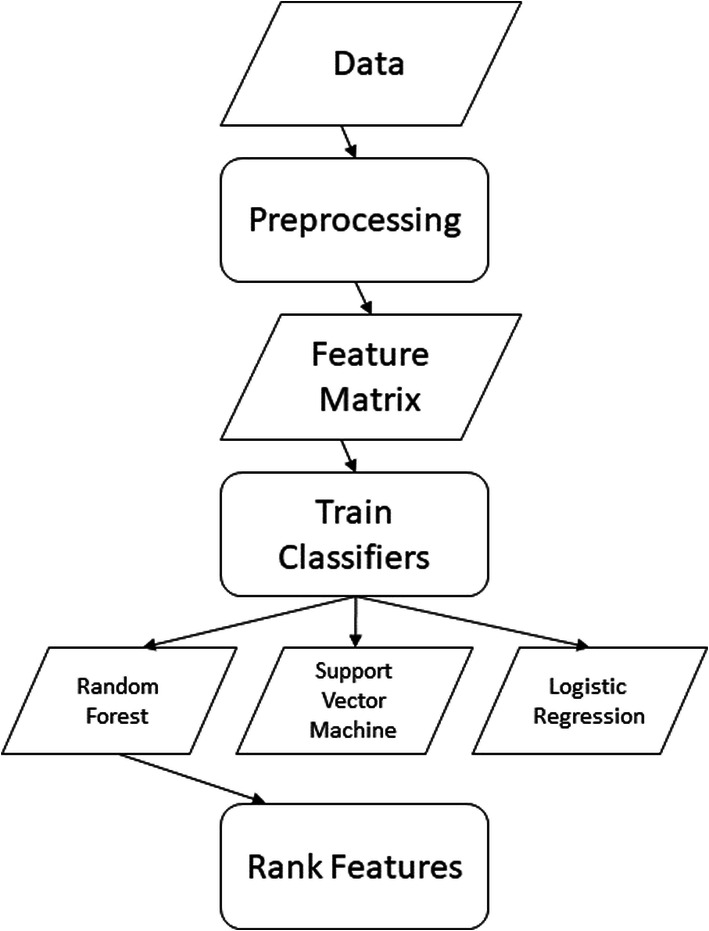
A flowchart of our analytics platform

The first step involves performing signal preprocessing for the following reasons. The libraries for the classification algorithms used here—logistic regression, random forests, and support vector machines—take training sets in the form of matrices, where each row corresponds to a subject and each column corresponds to a feature. Unfortunately, the original representation of each mass spectrum is a set of m/z values and their corresponding intensities. In addition, the intensities corresponding to specific m/z values in a mass spectrum can vary widely based on the intensity of the laser in the mass spectrometer for different measurements [28]. The practical implication is that relative frequencies within a mass spectrum may be more useful than the exact measurement of the intensity. Another potential problem is the alignment error along the m/z value axis [28], which often occurs in the measurement. Additionally, much of the MS literature focuses on peak finding [22]. On the other hand, our preprocessing algorithm performs feature extraction, i.e., extracting those expected to become important features for the classification.

There are three parameters used to control the peak extraction. The first parameter is the number of neighbors. For each m/z value, it specifies how many neighboring m/z values on each side to consider in the following way. If the intensity of any given m/z value is greater than the intensities of all its neighbors, then the given m/z value will be labeled as a peak; otherwise, it will not be labeled as a peak. The second parameter is the allowable misalignment error, denoted by ε, which provides correction for the possible misalignment along the m/z value axis. When a peak m/z value, denoted by m, is found, all the m/z values within [(1 − ε)m, (1 + ε)m] are also labeled as peaks. Finally, there is the minimum peak frequency. To the best of our knowledge, this is a parameter that has not been proposed in the literature. It specifies how often an m/z value must appear as a peak in all the samples in order to be labeled as a peak. Intuitively, this parameter allows for the removal of peaks that appear only in few samples due to the potential measurement errors.

Next, we provide more details on the preprocessing algorithm. To start the algorithm, each m/z value is rounded to the nearest integer. As a result, each subject’s mass spectrum is reduced to a vector of integers. Then, the algorithm identifies the peaks among all elements in the vector based on the number of neighbors. The algorithm iterates through the peak m/z values, adding other m/z values that should also be labeled as peaks, based on the allowable misalignment error. The peak m/z values identified from different subjects are combined to form a data matrix. Each row in the resultant matrix corresponds to a subject. Each column in the matrix corresponds to a unique m/z value that appears in one or many subjects’ peak m/z value lists. The m/z value is labeled as a peak (i.e., “T”) if it is a peak on the corresponding subject’s mass spectrum. The resultant matrix is a Boolean matrix. The algorithm removes columns in which the entry “T” does not appear often among the subjects, i.e., not in as many subjects as the total number of subjects multiplied by the minimum peak frequency. Finally, we replace the Boolean values in the matrix with the true intensities. The result of the preprocessing is a tunable feature selection process designed with mass spectrometry issues in mind (see Fig. 2 for the illustration of the preprocessing).

Fig. 2.

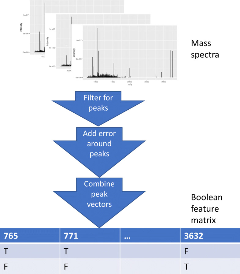
The preprocessing

After performing the preprocessing, the analysis platform inputs the matrix to perform binary classification on the number of days a blood sample has been stored at either temperature. We used three libraries in R, namely glmnet, randomForest, and e1071, to construct the LASSO-penalized logistic, random forest, and support vector machine binary classifiers, respectively. The reasons for these three choices are as follows. Logistic regression is one of the simplest classification techniques, resulting in a linear decision boundary, where the LASSO adds an L1 penalty on the coefficients [21]. The regularizer yields smaller coefficients in the linear decision boundary and encourages sparsity. To compare the linear classification to more expressive models, we also used random forests and support vector machines. Random forests integrate multiple decision trees, which results in a grid-like decision boundary. Our support vector machines used a radial basis kernel, which projects the data into a higher dimensional space before classification, thus allowing nonlinear decision boundaries [4]. The loss functions for each classifier were different. In the case of logistic regression, the loss function was the negative log likelihood of the data given the parameters plus a penalty on the L₁ norm of the coefficients. For the support vector machine, the loss function was the negative squared L₂ norm of the coefficients (which is equivalent to the negative margin of the separating hyperplane) plus a regularization term. Finally, for random forests, the loss was expected misclassification error (estimated using the bootstrap [5].)

For the logistic classifier, we tuned the λ parameter, which penalizes the L₁ norm of the weights, using cv.glmnet() function. For the random forest, we used the function tune.randomforest() to determine the appropriate number of features at each split in the tree for bootstrapping, which yielded a minimal out-of-bag error. For the support vector machine, we utilized the tune.svm() function to choose the appropriate γ and cost parameters for the radial kernel, which respectively are used to scale the distance between points and regularize soft-margin classification. Increasing gamma leads to interpreting points as less close, and increasing the cost increases the penalty on SVMs that misclassify points. To choose these parameters, we used leave-one-out cross-validation and performed exhaustive search with candidate values cost = 2⁻⁵, 2⁻³, 2⁻¹,…, 2⁵ and γ = 2⁻⁹, 2⁻⁷, 2⁻⁵,…, 2³.

After optimizing the hyperparameters of the classifiers using cross-validation (on 80% of the original dataset) of the room temperature and 4° C, respectively, we assessed them on independent test sets. Note that there are twice as many measurements as there are blood samples, as we focus on two measurements for each sample. Also, note that three measurements from the second dataset are missing.

Finally, to rank features, we used mean decrease in Gini impurity, measured on the random forest classifier. The Gini impurity index is $G={\sum }_{i=1}^{n_c}{p}_i(1-p_i)$, where n_c is the number of classes (n_c = 2 in our case) and p_i is the ratio of class. To compute the importance of a feature, we took the average of the importance of each split involving the feature, i.e., I = G_p − G_l − G_r, where G_p, G_l, and G_r are the Gini impurity indices for the parent, the left child, and the right child of the split, respectively [19].

Proof-of-Concept Study

In this section, we first investigate the relationship between the preprocessing algorithm parameters and the number of features extracted, and how changing the parameter values may affect the classification accuracy. We then report the results of applying logistic regression, support vector machines, and random forests to develop binary classifiers for the temporary classification problem. Our results help establish the validity of the logistic regression and random forest classifiers. Finally, we compare several feature ranking methods, including the use of random forest’s mean decrease in Gini impurity.

Analyzing the Preprocessing Parameters

In this section, we mainly focus on the relationship between the minimum peak frequency and the number of features identified. In addition, we briefly mention the impact of the other two preprocessing algorithm parameters.

Overall, our results indicate a few different relationships between preprocessing parameters and the number of features, as seen in Fig. 3. First, increasing the minimum peak frequency decreases the number of features identified for classification. Second, increasing the minimum peak frequency decreases the number of features, but in a nonlinear fashion. Third, increasing the neighbor parameter decreases the number of features. Finally, increasing the allowable misalignment error will increase the number of features.

Fig. 3.

The relationship between the preprocessing parameters and the number of features

Choosing good preprocessing parameters may not be an easy task. For example, choosing a small value for the number of neighbors may result in the inclusion of relatively unimportant features, while a large value may exclude an important m/z value if it lies near another high-intensity m/z value. Similarly, picking too small a misalignment error can lead to misinterpretation of data due to incorrect calibration of the mass spectrometer, while too large a value can create false peaks in the dataset.

Results Using the Binary Classifiers

Recall that we compared the performance of three classifiers: logistic regression, support vector machines, and random forests, with a variety of preprocessing parameters. The results were quite interesting. The room temperature dataset proved more difficult to classify than the 4 °C dataset for all three classifiers. However, logistic regression and random forest classifiers did quite well on each. The best performances on the independent test set for logistic regression and random forests on the room temperature dataset, respectively, were accuracies of 95 and 93%, while support vector machines only achieved a 79% accuracy. It is quite possible that this is due to overfitting. We compared this to a baseline approach of linearly interpolating intensity values, which is a version of smoothing, a popular recommendation in the literature. The baseline approach resulted in accuracies of 92 and 88% for logistic regression and random forests, and an accuracy of only 44% for support vector machines. An intuitive explanation is that linear separation of the data or classifying using a sequence of choices over different features is a simpler way to classify this data than projecting the data to a higher dimensional space and then classifying it in that space.

The best performances on the test sets in the 4° dataset were 99% for logistic regression, 76% for support vector machines, and 100% for random forests. The baseline approach resulted in accuracies of 97 and 100% for logistic regression and random forests, and a 76% accuracy for support vector machines. The excellent accuracies from random forests and logistic regression occurred with many different preprocessing parameters, which suggests that the 4 °C dataset was relatively easy to classify. It is unclear why 4 °C data were easier to classify than room temperature data. A possible explanation is that the setup on the mass spectrometer on the second day was significantly different than on the first day for the 4°C dataset. Another is that the degradation of the samples at 4 °C is in some way more consistent among samples, making them easier to classify.

The preprocessing parameters on the 4 °C dataset were almost meaningless since the data was so easy to classify. In fact, for 55 of the 144 different parameter experiments, logistic regression achieved 99% accuracy, and random forests achieved 100% accuracy in every experiment. However, on the room temperature dataset, the preprocessing parameters caused significant changes in classification accuracy. The best was a minimum peaks percentage of 15%, 11 neighbors, and an allowable misalignment error of 0.3%, which led to the best accuracy, 95%, for logistic regression. The worst was a minimum peaks percentage of zero, 5 neighbors, and an error window of 0.4%, which led to a 90% accuracy, likely due to the lack of feature selection. We suggest that the 11 neighbors’ setting is successful because it strongly selects for peaks in the mass spectra. In addition, making sure that only peaks showed up in a reasonably large fraction of the training samples (15%) meant that there was less potential for the classifier to overfit on an unimportant feature. Finally, having the nonzero error window parameter results in a correction for m/z axis misalignment error. It is reasonable to suppose that these parameters should be tuned when being used on a new dataset, but the parameters chosen here make intuitive sense.

Ranking the Identified Features

To rank the identified features, we used the mean decrease in Gini impurity, which can be computed using a random forest classifier. The random forest classifier was built using the best preprocessing parameter setting according to our tests, but with the allowable misalignment error of zero to avoid false peaks. For the room temperature data, the number of neighbors was set to be 11 and the minimum peak frequency was set to be 0.15. For the 4° C data, the number of neighbors was set to be 11 and the minimum peak frequency was set to be 0.25. The top features and their importance rankings are shown in Table 1. The top row presents the top-ranked m/z values, and the bottom row presents the corresponding mean decreases in Gini importance.

Table 1.

m/z values with the highest mean decrease in Gini impurity

Room temperature
1562	1318	3262	2022	1489	787	1490	1572	1324	1491	979	1206	1461	1091	1984	1556	1426	1237	803	1177
17	4.6	3.8	2.9	2.7	2.3	1.8	1.7	1.4	1.3	1.3	1.3	1.2	1.2	1.2	1	0.9	0.9	0.8	0.8
4° C temperature
1532	1531	1390	1562	1350	1461	1349	3264	1741	921	1289	830	1985	905	852	1044	1099	808	888	1061
16.4	8.9	7.3	7.3	7.1	3.1	2.8	2.1	1.1	0.8	0.6	0.6	0.5	0.4	0.4	0.4	0.3	0.3	0.2	0.2

Figure 4 further shows how well these top-ranked features separate the mass spectra. The m/z values 1531 and 1532 are very close, which suggests that a change in the alignment of the m/z value axis between measurements could have led to easy classification. Hence, we instead used the third and fourth most important features in the ranking. The results suggest that 4° C points are linearly separable, whereas the room temperature points are not. This difference mirrors the lower classification accuracies for the room temperature data. As evident in Fig. 4, 4° C data can be separated by just two important biomarkers, namely m/z values 1390 and 1562. Based on Fig. 4, it seems that mean decrease in Gini impurity is a strong indicator of variable importance.

Fig. 4.

The intensities associated with the two most important features (according to mean decrease in Gini impurity)

Conclusions

Based on our proof-of-concept study, we believe that aided by an enhanced peak extraction algorithm, both logistic regression and random forests are promising methods for classifying MALDI-based MS data. Our main finding is that, after parameter tuning, both classifiers perform temporal classification with 90+% accuracy. Additionally, mean decrease in Gini impurity appears to be effective in identifying MS-based proteomic biomarkers. Such biomarker identification can lead to labor- and cost-effective quality assessment tests in the future. We hope to see the analysis platform presented in this paper applied in other contexts, such as disease diagnosis, drug development, and food safety assessment.

Appendix

Before storage, the samples were left at room temperature for 1 h in order to allow coagulation and then centrifuged at 4° C for 15 min at 1400×g. In order to avoid fluid in the buffy-coat layer, serum was aspirated and collected in polypropylene tubes. After aliquoting, the samples were then stored in one of two conditions, room temperature or 4° C. For both cohorts, each sample’s mass spectrometer data was collected the day the sample was taken and then 1, 2, 5, and 10 days after that. This data was collected using a 1-μL sample that was processed by a mesoporous silicon wafer that was prepared by pre-baking in an oven at 120° C. This sample was spotted on the MALDI target plate and then allowed to air-dry. Afterwards, a 1-μL matrix in 50% acetonitrile containing 0.1% TFA was spotted on the dried sample spot. This sample was allowed to co-crystallize. The mass spectrum data was obtained by using a SHIMADZU AXIMA Resonance MALDI-IT-TOF equipped with a nitrogen laser emitting light at 337 nm. It had an adjustable mass range of 800 to 4000 Da. The positive ion was detected under reflective mode. After taking 500 laser shots, the spectra were usually averaged to find the final sample spectrum. The optimized accelerating voltage was 50 kV.

Funding Information

This study received financial support from NSF grant DMS#1246818 and an industry grant from the Chinese Academy of Sciences Holding Co., Ltd.

References

- 1.Ayache Saleh, Panelli Monica, Marincola Francesco M., Stroncek David F. Effects of Storage Time and Exogenous Protease Inhibitors on Plasma Protein Levels. American Journal of Clinical Pathology. 2006;126(2):174–184. doi: 10.1309/3WM7XJ7RD8BCLNKX. [DOI] [PubMed] [Google Scholar]
- 2.Baggerly KA, Morris JS, Coombes KR. Reproducibility of SELDI-TOF protein patterns in serum: comparing datasets from different experiments. Bioinformatics. 2004;20(5):777–785. doi: 10.1093/bioinformatics/btg484. [DOI] [PubMed] [Google Scholar]
- 3.Ball G, et al. An integrated approach utilizing artificial neural networks and SELDI mass spectrometry for the classification of human tumours and rapid identification of potential biomarkers. Bioinformatics. 2002;18(3):395–404. doi: 10.1093/bioinformatics/18.3.395. [DOI] [PubMed] [Google Scholar]
- 4.Bishop CM. Pattern recognition and machine learning (information science and statistics) Secaucus: Springer-Verlag New York, Inc.; 2006. [Google Scholar]
- 5.Breiman L. Bagging predictors. Mach Learn. 1996;24(2):123–140. [Google Scholar]
- 6.Carvalho PC, et al. Identifying differences in protein expression levels by spectral counting and feature selection. Genet Mol Res. 2008;7(2):342. doi: 10.4238/vol7-2gmr426. [DOI] [PMC free article] [PubMed] [Google Scholar]
- 7.Chaigneau C, et al. Serum biobank certification and the establishment of quality controls for biological fluids: examples of serum biomarker stability after temperature variation. Clin Chem Lab Med. 2007;45(10):1390–1395. doi: 10.1515/CCLM.2007.160. [DOI] [PubMed] [Google Scholar]
- 8.Datta S, DePadilla LM. Feature selection and machine learning with mass spectrometry data for distinguishing cancer and noncancer samples. Stat Methodol. 2006;3(1):79–92. doi: 10.1016/j.stamet.2005.09.006. [DOI] [Google Scholar]
- 9.Jackson DH, Banks RE. Banking of clinical samples for proteomic biomarker studies: a consideration of logistical issues with a focus on pre-analytical variation. Proteomics Clin Appl. 2010;4(3):250–270. doi: 10.1002/prca.200900220. [DOI] [PubMed] [Google Scholar]
- 10.Jenkins MA. Quality control and quality assurance aspects of the routine use of capillary electrophoresis for serum and urine proteins in clinical laboratories. Electrophoresis. 2004;25(10–11):1555–1560. doi: 10.1002/elps.200405882. [DOI] [PubMed] [Google Scholar]
- 11.Kozak KR, et al. Identification of biomarkers for ovarian cancer using strong anion-exchange ProteinChips: potential use in diagnosis and prognosis. Proc Natl Acad Sci. 2003;100(21):12343–12348. doi: 10.1073/pnas.2033602100. [DOI] [PMC free article] [PubMed] [Google Scholar]
- 12.Levner I. Feature selection and nearest centroid classification for protein mass spectrometry. BMC Bioinformatics. 2005;6(1):1. doi: 10.1186/1471-2105-6-68. [DOI] [PMC free article] [PubMed] [Google Scholar]
- 13.Liang K, et al. Mesoporous silica chip: enabled peptide profiling as an effective platform for controlling bio-sample quality and optimizing handling procedure. Clin Proteomics. 2016;13(1):34. doi: 10.1186/s12014-016-9134-9. [DOI] [PMC free article] [PubMed] [Google Scholar]
- 14.Ostroff R, et al. The stability of the circulating human proteome to variations in sample collection and handling procedures measured with an aptamer-based proteomics array. J Proteomics. 2010;73(3):649–666. doi: 10.1016/j.jprot.2009.09.004. [DOI] [PubMed] [Google Scholar]
- 15.Papadopoulos MC, et al. A novel and accurate diagnostic test for human African trypanosomiasis. Lancet. 2004;363(9418):1358–1363. doi: 10.1016/S0140-6736(04)16046-7. [DOI] [PubMed] [Google Scholar]
- 16.Petricoin EF, et al. Use of proteomic patterns in serum to identify ovarian cancer. Lancet. 2002;359(9306):572–577. doi: 10.1016/S0140-6736(02)07746-2. [DOI] [PubMed] [Google Scholar]
- 17.Pieragostino Damiana, Petrucci Francesca, Del Boccio Piero, Mantini Dante, Lugaresi Alessandra, Tiberio Sara, Onofrj Marco, Gambi Domenico, Sacchetta Paolo, Di Ilio Carmine, Federici Giorgio, Urbani Andrea. Pre-analytical factors in clinical proteomics investigations: Impact of ex vivo protein modifications for multiple sclerosis biomarker discovery. Journal of Proteomics. 2010;73(3):579–592. doi: 10.1016/j.jprot.2009.07.014. [DOI] [PubMed] [Google Scholar]
- 18.Rai AJ, et al. HUPO Plasma Proteome Project specimen collection and handling: towards the standardization of parameters for plasma proteome samples. Proteomics. 2005;5(13):3262–3277. doi: 10.1002/pmic.200401245. [DOI] [PubMed] [Google Scholar]
- 19.Russell SJ, et al. Artificial intelligence: a modern approach. Vol. 2. Upper Saddle River: Prentice hall; 2003. [Google Scholar]
- 20.Sorace JM, Zhan M. A data review and re-assessment of ovarian cancer serum proteomic profiling. BMC Bioinformatics. 2003;4(1):1. doi: 10.1186/1471-2105-4-24. [DOI] [PMC free article] [PubMed] [Google Scholar]
- 21.Tibshirani Robert. Regression Shrinkage and Selection Via the Lasso. Journal of the Royal Statistical Society: Series B (Methodological) 1996;58(1):267–288. [Google Scholar]
- 22.Tibshirani R, et al. Sample classification from protein mass spectrometry, by ‘peak probability contrasts’. Bioinformatics. 2004;20(17):3034–3044. doi: 10.1093/bioinformatics/bth357. [DOI] [PubMed] [Google Scholar]
- 23.Veenstra TD, et al. Biomarkers: mining the biofluid proteome. Mol Cell Proteomics. 2005;4(4):409–418. doi: 10.1074/mcp.M500006-MCP200. [DOI] [PubMed] [Google Scholar]
- 24.Villanueva J, Philip J, Chaparro CA, Li Y, Toledo-Crow R, DeNoyer L, Fleisher M, Robbins RJ, Tempst P. Correcting common errors in identifying cancer-specific serum peptide signatures. J Proteome Res. 2005;4(4):1060–1072. doi: 10.1021/pr050034b. [DOI] [PMC free article] [PubMed] [Google Scholar]
- 25.Wagner M, Naik D, Pothen A. Protocols for disease classification from mass spectrometry data. Proteomics. 2003;3(9):1692–1698. doi: 10.1002/pmic.200300519. [DOI] [PubMed] [Google Scholar]
- 26.Won Y, et al. Pattern analysis of serum proteome distinguishes renal cell carcinoma from other urologic diseases and healthy persons. Proteomics. 2003;3(12):2310–2316. doi: 10.1002/pmic.200300590. [DOI] [PubMed] [Google Scholar]
- 27.Wu B, et al. Comparison of statistical methods for classification of ovarian cancer using mass spectrometry data. Bioinformatics. 2003;19(13):1636–1643. doi: 10.1093/bioinformatics/btg210. [DOI] [PubMed] [Google Scholar]
- 28.Yasui Y, et al. A data-analytic strategy for protein biomarker discovery: profiling of high-dimensional proteomic data for cancer detection. Biostatistics. 2003;4(3):449–463. doi: 10.1093/biostatistics/4.3.449. [DOI] [PubMed] [Google Scholar]
- 29.Yu JS, et al. Ovarian cancer identification based on dimensionality reduction for high-throughput mass spectrometry data. Bioinformatics. 2005;21(10):2200–2209. doi: 10.1093/bioinformatics/bti370. [DOI] [PubMed] [Google Scholar]
- 30.Zhang X, et al. Recursive SVM feature selection and sample classification for mass-spectrometry and microarray data. BMC Bioinformatics. 2006;7(1):1. doi: 10.1186/1471-2105-7-1. [DOI] [PMC free article] [PubMed] [Google Scholar]