

Introduction
Electronic health records (EHR) consisting of the medical history of patients are useful in various clinical applications such as diagnosis and recommending medicine [22]. Traditional machine learning approaches often require careful domain-specific feature engineering to achieve good prediction performance. On the other hand, deep learning approaches enable end-to-end learning without the need of hand-crafted and domain-specific features, and have recently produced promising results for various clinical prediction tasks [17, 22, 29]. As a result, there has been a rapid growth in the applications of deep learning to various clinical prediction tasks from electronic health records, e.g., Doctor AI [6] for medical diagnosis, Deep Patient [21] to predict future diseases in patients, and DeepR [23] to predict unplanned readmission after discharge. With various medical parameters being recorded over a period of time in EHR databases, recurrent neural networks (RNNs) can be an effective way to model the sequential aspects of EHR data and, in turn, enable applications in diagnoses [3, 6, 17], mortality prediction, and estimating length of stay [9, 27, 28].
However, like most deep learning approaches, RNNs are prone to overfitting when labeled training data is scarce, and often require careful and computationally expensive hyper-parameter tuning effort. Transfer learning [2, 24] is known to mitigate this: It enables knowledge transfer from neural networks trained on a source task (domain) with sufficient training instances to a related target task (domain) with few training instances. For example, training a deep network on a diverse set of images can provide useful features for images from unseen domains [31]. Moreover, fine-tuning a pre-trained network for the target task is often faster and easier than constructing and training a new network from scratch [2, 19].
It has been shown that pre-trained networks can learn to extract a rich set of generic features that can then be applied to a wide range of other similar tasks [19]. Also, it has been argued that transferring weights even from distant tasks can be better than using random initial weights in neural networks [35]. Transfer learning via fine-tuning parameters of pre-trained models for end tasks has been recently considered for medical applications as well [6, 16]. However, fine-tuning a large number of parameters with a small-labeled dataset may still result in overfitting, and requires careful regularization (as we show in Section 9 through empirical evaluation). In this work, we consider two simple yet effective approaches to transfer the knowledge captured in pre-trained deep RNNs for new target tasks in healthcare domain. More specifically, we consider two scenarios: (i) extract features from a pre-trained network and use them to build models for target task and (ii) initialize deep network for target task using parameters of a pre-trained network and then fine-tune using labeled training data for target task.
The key contributions of this work are:
We propose two approaches for transfer learning for classification tasks such as patient phenotyping and mortality prediction given multivariate time series corresponding to physiological parameters of patients1. For a target task in the healthcare domain, we consider (i) a domain adaptation approach using a general-purpose off-the-shelf time series feature extractor based on deep RNN, to remove the effort and resources required to train a deep network from scratch while still leveraging its advantages, and (ii) a task adaptation approach based on a deep RNN trained using labeled data from another set of (source) tasks in healthcare domain to reduce the dependence on labeled training data for the target task and also reduce hyper-parameter tuning effort.
Our proposed approaches allow extracting robust features from variable length multivariate time series by using pre-trained deep RNNs, thereby reducing dependence on expert domain-driven feature extraction.
We show that carefully regularized fine-tuning of pre-trained RNNs leads to models that are significantly more robust to training data size in comparison with task-specific classification models trained from scratch.
We also study the trade-off between domain adaptation and task adaptation with respect to the amount of labeled data from the healthcare domain, and show that leveraging pre-trained models from other (seemingly unrelated) domains can be useful in scenarios where task adaptation may be ineffective, e.g., when labeled data for the target task as well as its related tasks within the healthcare domain is scarce.
Through empirical evaluation of patient phenotyping and mortality prediction tasks on MIMIC-III benchmark dataset [13], we demonstrate that our transfer learning approaches yield data- and compute-efficient classification models that require little training or fine-tuning effort while yielding classification performance that is comparable with models with hand-crafted features or carefully trained domain-specific deep networks benchmarked in [9, 10, 32].
The rest of the paper is organized as follows: In Section 2, we present related work, and provide details of an existing off-the-shelf pre-trained deep RNN, namely TimeNet [19], in Section 3. We provide an overview of the proposed domain and task adaptation approaches in Section 4, followed by their details in Sections 5 and 6, respectively. In Section 7, we provide details of cohort selection and datasets. We provide experimental details and observations in Sections 8 and 9, respectively, and comparison of two approaches in Section 10, and finally conclude in Section 11.
Related Work
TimeNet-based features have been shown to be useful for various tasks including ECG classification [19]. In this work, we consider application of TimeNet to phenotyping and in-hospital mortality tasks for multivariate clinical time series classification. Deep Patient [21] proposes leveraging features from a pre-trained stacked-autoencoder for EHR data. However, it does not leverage the temporal aspect of the data and uses a non-temporal model based on stacked-autoencoders. Our domain adaptation approach extracts temporal features via TimeNet while incorporating the important sequential nature of EHR data. Doctor AI [6] uses discretized medical codes (e.g., diagnosis, medication, procedure) from longitudinal patient visits via a purely supervised setting while we use real-valued time series. While approaches like Doctor AI require training a deep RNN from scratch, our approach leverages a general-purpose RNN for feature extraction.
Harutyunyan et al. [9] consider training a deep RNN model under multitask learning setting (for multiple prediction tasks including phenotyping and in-hospital mortality) to learn a general-purpose deep RNN for clinical time series. They show that it is possible to train a single network for multiple tasks simultaneously by capturing generic features that work across different tasks. We also consider leveraging generic features for clinical time series but under the transfer learning setting where we pre-train an RNN on different domains or set of different tasks. This pre-training allows our approach to be more data and resource efficient.
Unsupervised pre-training has been shown to be effective in capturing the generic patterns and distribution from EHR data [21]. Further, RNNs for time series classification from EHR data have been successfully explored, e.g., in [3, 17]. However, these approaches do not address the challenge posed by limited labeled data, which is the focus of this work. Transfer learning using deep neural networks has been recently explored for medical applications: A model learned from one hospital could be adapted to another hospital for the same task via RNNs [6]. A deep neural network was used to transfer knowledge from one dataset to another while the source and target tasks (named-entity recognition from medical records) are the same in [16]. However, in both these transfer learning approaches, the source and target tasks are the same while only the dataset changes. In contrast, our task adaptation approach allows to transfer the model trained on several healthcare-specific tasks to a different (although related) classification task using RNNs for clinical time series.
Background: TimeNet
Deep (multi-layered) RNNs have been shown to perform hierarchical processing of time series with different layers tackling different time scales [11, 18]. TimeNet [19] is a general-purpose multi-layered RNN trained on large number of diverse univariate time series from UCR Time Series Archive [4] that has been shown to be useful as off-the-shelf feature extractor for time series. TimeNet has been trained on 18 different datasets simultaneously via an RNN autoencoder in an unsupervised manner for reconstruction task. Features extracted from TimeNet have been found to be useful for classification task on 30 datasets from various domains not seen during training of TimeNet, proving its ability to provide meaningful features for unseen datasets.
TimeNet contains three recurrent layers having 60 gated recurrent units (GRUs) [5] each. TimeNet is an RNN trained via an autoencoder consisting of an encoder RNN and a decoder RNN trained simultaneously using the sequence-to-sequence learning framework [1, 33] as shown in Fig. 1. RNN autoencoder is trained to obtain the parameters WE of the encoder RNN fE via reconstruction task such that for input x1…τ = x1, x2,..., xτ (), the target output time series xτ…1 = xτ, xτ− 1,..., x1 is reverse of the input.
Fig. 1.

a TimeNet trained via RNN Encoder-Decoder with three hidden GRU layers. b TimeNet-based feature extraction. TimeNet is shown unrolled for L = 3
The RNN encoder fE provides a non-linear mapping of the univariate input time series to a fixed-dimensional vector representation zτ: zτ = fE(x1…τ;WE), followed by an RNN decoder fD based non-linear mapping of zτ to univariate time series: ; where WE and WD are the parameters of the encoder and decoder, respectively. The model is trained to minimize the average squared reconstruction error. Training on 18 diverse datasets simultaneously results in robust time series features getting captured in zτ: the decoder relies on zτ as the only input to reconstruct the time series, forcing the encoder to capture all the relevant information in the time series into the fixed-dimensional vector zτ. This vector zτ is used as the feature vector for input x1…τ. This feature vector is then used to train a simpler classifier (e.g., SVM, as used in [19]) for the end task. TimeNet maps a univariate input time series to 180-dimensional feature vector, where each dimension corresponds to final output of one of the 60 GRUs in the 3 recurrent layers.
Approach Overview
Consider sets and of time series instances corresponding to a source (S) and a target (T) dataset, respectively. , where NS is the number of time series instances in the source dataset. Denoting time series by x and the corresponding target label by y for simplicity of notation, we have x = x1, x2,…xτ denote a time series of length τ, where (t = 1…τ) is an n-dimensional vector corresponding to n parameters. Further, , where K is the number of binary classification tasks. Similarly, such that NT ≪ NS, and such that the target task is a binary classification task. We consider and to be from same (different) domain if the n parameters in and are the same (different). Further, we consider the tasks for and to be the same if number of target classes in yS and yT is same and the corresponding classes are semantically same, for example, both yS and yT contain two classes {patient survives, patient dies}.
We consider two scenarios for transfer learning using RNNs:
-
i)
Domain adaptation where contains time series from various domains such as electric devices, motion capture, spectrographs, sensor readings, ECGs, and simulated time series, taken from publicly available UCR Time Series Classification Archive [4], and contains clinical time series from EHR database (i.e., sets and are from different domains). We consider pre-training an RNN using via unsupervised learning and study its ability to compute useful features for time series from an unseen domain (healthcare in our case). We adapt pre-trained model using via supervised learning (Note: As we adapt model trained via unsupervised learning for supervised task, set and are from different task);
-
ii)
Task adaptation where both and contain time series from the healthcare domain such that the parameters in xS and xT correspond to the same n physiological parameters such as heart rate, pulse rate, and oxygen saturation. Further, yS corresponds to various tasks, such as presence/absence of phenotypes, e.g., acute cerebrovascular disease, diabetes mellitus with complications, and gastrointestinal hemorrhage, and yT corresponds to a related but different task, e.g., present/absence of new phenotypes that are not present in yS. We consider pre-training an RNN model using via supervised learning on the diverse set of tasks in yS such that the model learns to capture and extract a rich set of generic features from clinical time series that can be useful for other tasks in the same domain. We adapt the pre-trained model using via supervised learning.
Domain Adaptation: Adapting Universal Time Series Feature Extractors to Healthcare Domain
General-purpose time series feature extractors such as TimeNet [19] and Universal Encoder [30] usually constrain the input time series to be univariate as it is difficult to cater to multivariate time series with varying dimensionality in a single neural network. In this scenario, we consider adapting TimeNet to healthcare domain with two key considerations2: (i) extend TimeNet for multivariate clinical time series classification tasks that requires simultaneous consideration of various physiological parameters and (ii) adapt the features from TimeNet for specific tasks from healthcare such as patient phenotyping and mortality prediction tasks. We show how TimeNet can be adapted to these classification tasks by training computationally efficient traditional linear classifiers on top of features extracted for each parameter using TimeNet, as depicted in Fig. 2. Further, we propose a simple mechanism to leverage the weights of the trained linear classifier to provide insights into the relevance of each raw input feature (physiological parameter) for a given phenotype (described in Section 5.3).
Fig. 2.
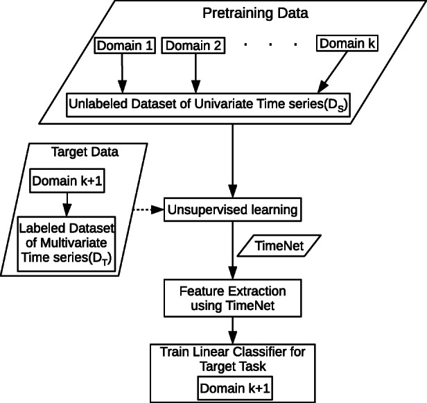
Domain adaptation scenario. TimeNet is pre-trained in an unsupervised manner on time series from k diverse domains, and then used to extract features from time series in (k + 1)-th domain for subsequent target classification task
Consider is set of labeled time series instances from an EHR database: , where is a multivariate time series, such that the target task is a binary classification task, NT is the number of time series instances corresponding to patients. We consider the presence or absence of a phenotype as a binary classification task and learn an independent model for each phenotype (unlike [9] which consider phenotyping as a multi-label classification problem). This allows us to build simple and compute-efficient linear binary classification models as described next. In practice, the outputs of these binary classifiers can then be considered together to estimate the set of phenotypes present in a patient. Similarly, mortality prediction is considered to be a binary classification task where the goal is to classify whether the patient will survive (after admission to ICU) or not.
Feature Extraction for Multivariate Clinical Time Series
For a multivariate time series x = x1, x2,…xτ, where , we consider time series for each of the n raw input features (physiological parameters, e.g., glucose level and heart rate) independently, to obtain univariate time series xj = xj1, xj2,…xjτ, where j = 1…n. (Note: We use x instead of x(i) and omit superscript (i) for ease of notation). We obtain the vector representation zjτ = fE(xj;WE) for xj using TimeNet, where with c = 180 (as described in Section 3). We concatenate the TimeNet-features zjτ for each raw input feature j to get the final feature vector zτ = [z1τ, z2τ,…, znτ] for time series x, where , m = n × c as illustrated in Fig. 3.
Fig. 3.

Domain adaptation. TimeNet-based feature extraction and classification
In general, time series length τ varies across instances, i.e., depends on i (e.g., based on length of stay in the hospital). We assume equal length for each time series for sake of clarity without loss of generality. In practice, we convert each time series to have equal length τ by suitable pre/post-padding with 0s.
Using TimeNet-Based Features for Classification
The final concatenated feature vector zτ is used as input to the phenotyping and mortality prediction classification models. We consider a linear mapping from input TimeNet features zτ to the target label y s.t. the estimate , where . We note that since c = 180 is large, zτ has large number of features m ≥ 180. We, therefore, constrain the linear model with weights w to use only a few of these large number of features. The weights are obtained using LASSO-regularized loss function [34]:
| 1 |
where y(i) ∈{0,1}, is the L1-norm, wjk represents the weight assigned to the k-th TimeNet feature for the j-th raw feature, and α controls the extent of sparsity with higher α implying more sparsity, i.e., fewer TimeNet features are implicitly used to arrive at the final classification decision.
Obtaining Relevance Scores for Raw Features
Determining relevance of the n raw input features for a given phenotype is potentially useful to obtain insights into the obtained classification model. The learned weights w are easy to interpret and can give interesting insights into relevant features for a classification task (e.g., as used in [20]). We obtain the relevance rj of the j-th raw input feature as the sum of the absolute values of the weights wjk assigned to the corresponding TimeNet features zjτ as shown in Fig. 4, s.t.
| 2 |
Further, rj is normalized using min-max normalization to obtain ; where and . In practice, these normalized relevance scores for the raw features help to interpret and validate the overall model. For example, one would expect blood glucose level raw input feature to have a high relevance score in the classification model learned to detect diabetes mellitus phenotype (we provide such insights later in Section 8).
Fig. 4.
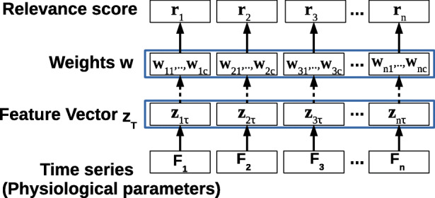
Obtaining relevance scores for raw input features. Here, τ time series length, n number of raw input features
Task Adaptation: Adapting Healthcare-Specific Pre-trained Models to a New Task
As depicted in Fig. 5, the goal of task adaptation is to transfer the learning from a set of source tasks to a related target task for clinical time series by means of an RNN. Considering phenotype detection from time series of physiological parameters as a binary classification task, we train HealthNet as an RNN classifier on a diverse set of such binary classification tasks simultaneously (one task per phenotype) using a large labeled dataset. We consider the following approaches to adapt it to an unseen target task:
Initialize parameters of the target task-specific RNN using the parameters of HealthNet previously trained on a large number of source tasks; so that HealthNet provides good initialization of parameters of task-specific RNN and train the model (described in Section 6.2).
Extract features using HealthNet and then learn an easily trainable non-temporal linear classification model such as a logistic regression model [12] for target tasks with few labeled instances (described in Section 6.3).
Fig. 5.
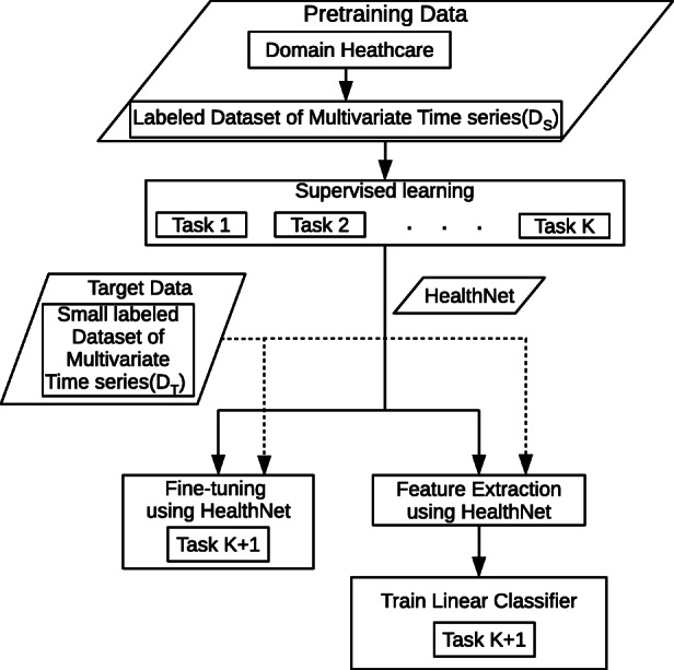
Task adaptation scenario. HealthNet is pre-trained for K classification tasks from healthcare domain simultaneously via supervised training. Then, it is adapted for target task either via fine-tuning or feature extraction (potentially using only a small amount of labeled training data for target task)
More specifically, consider and are sets of labeled time series instances from an EHR database (i.e., same domain): , where is a multivariate time series, , K is the number of binary classification tasks, and NS is the number of time series instances corresponding to patients. Similarly, such that NT ≪ NS, and such that the target task is a binary classification task. As depicted in Fig. 6a, we first train HealthNet on K source tasks using (refer to Section 6.1 for details), and then consider the following two scenarios for adapting to the pre-trained model to target tasks using :
Fine-tune the HealthNet with suitable regularization (refer Section 6.2 for details), as shown in Fig. 6b. This allows us to train a model that does not require hyper-parameter tuning efforts.
Train the simpler logistic regression (LR) classifier for target task and the features obtained via HealthNet (refer Section 6.3 for details), as shown in Fig. 7, which is compute-efficient.
We next provide details of training and fine-tuning the HealthNet and training the LR models.
Fig. 6.

a HealthNet trained via supervised learning for multiple source tasks simultaneously using final activation as sigmoid. b Fine-tuning HealthNet for a new target task using final activation as softmax. Here, blue and red arrows correspond to recurrent and feed forward weights of the recurrent layers, respectively. Only feed forward (red) weights are regularized while fine-tuning the HealthNet. RNN with L = 2 hidden layers is shown unrolled over τ = 3 time steps
Fig. 7.
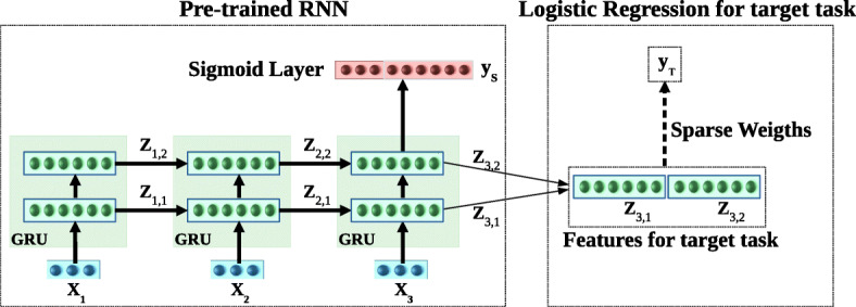
Inference in task adaptation. Using features extracted from HealthNet. RNN with L = 2 hidden layers is shown unrolled over τ = 3 time steps
Obtaining HealthNet Using Supervised Pre-training of RNN
Training an RNN on K binary classification tasks simultaneously can be considered as a multi-label classification problem. We train a multi-layered RNN with L recurrent layers having GRUs to map to y(i). Let denote the output of recurrent units in l-th hidden layer at time t, and denote the hidden state at time t obtained as concatenation of hidden states of all layers, where h is the number of GRU units in a hidden layer and m = h × L. The parameters of the network are obtained by minimizing the cross-entropy loss via stochastic gradient descent:
| 3 |
Here σ(x) = (1 + e−x)− 1 is the sigmoid activation function, is the estimate for target y(i), are parameters of recurrent layers, and WC and bC are parameters of the classification layer.
Fine-Tuning of HealthNet
We initialized the target task-specific RNN parameters by the pre-trained RNN parameters of recurrent layers () and a new binary classification layer parameters ( and ). We obtain probabilities of two classes for the binary classification task as = , where is the output of recurrent units in last layer (L) at last timestamp (τ). Let and are feed forward and recurrent weights of the recurrent layers. All parameters are trained together by minimizing cross-entropy loss with regularizer. We consider two regularizer techniques to obtain two different fine-tuned models with loss given by and via stochastic gradient descent:
| 4 |
| 5 |
where is the probability of positive class, is the L1 norm with λ controlling the extent of sparsity, and is the L2 norm. As [25] suggests that using an L1 or L2 penalty on the recurrent weights compromises the ability of the network to learn and retain information through time, therefore, we apply L1 or L2 regularizer only to the feed forward connections across recurrent layers and not the weights of the recurrent connections.
LR Models Using Features Extracted from HealthNet
For input , the hidden state at last time step τ is used as input feature vector for training the LR model. We obtain probability of the positive class for the binary classification task as = , where , are parameters of LR. The parameters are obtained by minimizing the negative log-likelihood loss :
| 6 |
where is the L1 regularizer with λ controlling the extent of sparsity—with higher λ implying more sparsity, i.e., fewer features from the representation vector are selected for the final classifier. It is to be noted that this way of training the LR model on pre-trained RNN features is equivalent to freezing the parameters of all the hidden layers of the pre-trained RNN while tuning the parameters of a new final classification layer which has been used successfully in, e.g., [14]. The sparsity constraint ensures that only a small number of parameters are to be tuned which is useful to avoid overfitting when labeled data is small.
Dataset Description
We use MIMIC-III (v1.4) clinical database [13] which consists of over 60,000 ICU stays across 40,000 critical care patients. We use the same experimental setup as in [9], with same splits and features for train, validation, and test datasets3 based on 17 physiological parameters with 12 real-valued (e.g., blood glucose level and systolic blood pressure) and 5 categorical time series (e.g., Glascow coma scale motor response and Glascow coma scale verbal), sampled at 1-h intervals. The categorical variables are converted to one-hot vectors such that the final multivariate time series has n = 76 raw input features (59 actual features and 17 masking features to denote missing values). Refer to Table 4 in the Appendix for names of raw features used. In all our experiments, we restrict training time series data up to first 48 h in ICU stay, such that τ = 48 with one reading every 1 h while training all models to imitate practical scenario where early predictions are important, unlike [9, 32] which use entire time series for training the classifier for phenotyping task. The benchmark dataset contains label information for presence/absence of 25 phenotypes common in adult ICUs (e.g., acute cerebrovascular disease, diabetes mellitus with complications, and gastrointestinal hemorrhage), and in-hospital mortality, whether the patient survived or not after ICU admission (class 1: patient dies, class 0: patient survives).
Table 4.
List of raw input features
| 1 | Glucose | 31 | Glascow coma scale eye opening → 3 to speech |
| 2 | Glascow coma scale total → 7 | 32 | Height |
| 3 | Glascow coma scale verbal response → incomprehensible sounds | 33 | Glascow coma scale motor response → 5 localizes pain |
| 4 | Diastolic blood pressure | 34 | Glascow coma scale total → 14 |
| 5 | Weight | 35 | Fraction inspired oxygen |
| 6 | Glascow coma scale total → 8 | 36 | Glascow coma scale total → 12 |
| 7 | Glascow coma scale motor response → obeys commands | 37 | Glascow coma scale verbal response → confused |
| 8 | Glascow coma scale eye opening → none | 38 | Glascow coma scale motor response → 1 no response |
| 9 | Glascow coma scale eye opening → to pain | 39 | Mean blood pressure |
| 10 | Glascow coma scale total → 6 | 40 | Glascow coma scale total → 4 |
| 11 | Glascow coma scale verbal response → 1.0 ET/Trach | 41 | Glascow coma scale eye opening → to speech |
| 12 | Glascow coma scale total → 5 | 42 | Glascow coma scale total → 15 |
| 13 | Glascow coma scale verbal response → 5 oriented | 43 | Glascow coma scale motor response → 4 flex-withdraws |
| 14 | Glascow coma scale total → 3 | 44 | Glascow coma scale motor response → no response |
| 15 | Glascow coma scale verbal response → no response | 45 | Glascow coma scale eye opening → spontaneously |
| 16 | Glascow coma scale motor response → 3 abnorm flexion | 46 | Glascow coma scale verbal response → 4 confused |
| 17 | Glascow coma scale verbal response → 3 inapprop words | 47 | Capillary refill rate → 0.0 |
| 18 | Capillary refill rate → 1.0 | 48 | Glascow coma scale total → 13 |
| 19 | Glascow coma scale verbal response → inappropriate words | 49 | Glascow coma scale eye opening → 1 no response |
| 20 | Systolic blood pressure | 50 | Glascow coma scale motor response → abnormal extension |
| 21 | Glascow coma scale motor response → flex-withdraws | 51 | Glascow coma scale total → 11 |
| 22 | Glascow coma scale total → 10 | 52 | Glascow coma scale verbal response → 2 incomp sounds |
| 23 | Glascow coma scale motor response → obeys commands | 53 | Glascow coma scale total → 9 |
| 24 | Glascow coma scale verbal response → no response-ETT | 54 | Glascow coma scale motor response → abnormal flexion |
| 25 | Glascow coma scale eye opening → 2 to pain | 55 | Glascow coma scale verbal response → 1 no response |
| 26 | Heart rate | 56 | Glascow coma scale motor response → 2 abnorm extensn |
| 27 | Respiratory rate | 57 | pH |
| 28 | Glascow coma scale verbal response → oriented | 58 | Glascow coma scale eye opening → 4 spontaneously |
| 29 | Glascow coma scale motor response → localizes pain | 59 | Oxygen saturation |
| 30 | Temperature |
The benchmark dataset contains label information for presence/absence of 25 phenotypes common in adult ICUs including 12 critical (and sometimes life-threatening) conditions, such as respiratory failure and sepsis; 8 chronic conditions that are common comorbidities and risk factors in critical care, such as diabetes and metabolic disorders; and 5 conditions considered “mixed” because they are recurring or chronic with periodic acute episodes. We also consider the task of predicting in-hospital mortality, i.e., whether the patient survived or not after ICU admission (class 1: patient dies, class 0: patient survives).
We use the same evaluation metrics and protocol as in [9, 10] unless mentioned otherwise, including macro- and micro-averaged AUROC for phenotyping task, and AUROC and AUPRC for in-hospital mortality prediction task, where AUROC (area under the receiver operator characteristic curve) is the commonly used metric in classification tasks, micro AUROC is calculated by single AUROC computed on flattened model prediction and ground truth matrices, micro AUROC calculated by averaging performance metric per-class/label. AUPRC (area under the precision-recall curve) better suits to problems with imbalanced classes which happens to be the case here for both phenotyping and in-hospital mortality tasks, e.g., 4493 (10.63%) out of 42,276 patients died in-hospital making in-hospital mortality prediction task to have high class imbalance.
Experimental Evaluation for Domain Adaptation
We evaluate TimeNet-based transfer learning approach on binary classification tasks (i) presence/absence of 25 phenotypes and (ii) in-hospital mortality task.
Experimental Setup
We have n = 76 raw input features resulting in m = 13,680-dimensional (m = 76 × 180) TimeNet feature vector for each admission. We use α = 0.0001 for phenotype classifiers and use α = 0.0003 for in-hospital mortality classifier (α is chosen based on hold-out validation set). Table 1 summarizes the results of phenotyping and in-hospital mortality prediction task, and provides comparison with existing benchmarks. Refer to Table 3 in the Appendix for detailed phenotype-wise results. We report the values of the performance metrics for all models along with 95% confidence intervals obtained by resampling the test set 10,000 times with replacement.
Table 1.
Classification performance comparison of TimeNet-based models with LR (logistic regression model over manually designed statistical features) and LSTM (LSTM classifier trained from scratch) for the phenotyping and in-hospital mortality prediction tasks
| Phenotyping task | ||
| approach | Micro AUROC | Macro AUROC |
| LR | 0.799 (0.796, 0.803) | 0.739 (0.734, 0.743) |
| LSTM | 0.821 (0.818, 0.825) | 0.770 (0.766, 0.775) |
| TimeNet-48 | 0.812 (0.808, 0.815) | 0.761 (0.757, 0.765) |
| TimeNet-All | 0.813 (0.810, 0.817) | 0.764 (0.759, 0.768) |
| TimeNet-48-Eps | 0.820 (0.817, 0.824) | 0.772 (0.768, 0.777) |
| TimeNet-All-Eps | 0.822 (0.819, 0.825) | 0.775 (0.771,0.779) |
| In-hospital mortality prediction task | ||
| approach | AUROC | AUPRC |
| LR | 0.848 (0.828, 0.868) | 0.474 (0.419, 0.529) |
| LSTM | 0.855 (0.835, 0.873) | 0.485 (0.431, 0.537) |
| TimeNet-48 | 0.852 (0.831, 0.872) | 0.519 (0.467, 0.571) |
Numbers in round brackets denote 95% confidence intervals. Here, results of LR and LSTM are taken from [10] (Note: For phenotyping, we compare TimeNet-48-Eps with existing benchmarks over TimeNet-All-Eps as it is more applicable in practical scenarios. Only TimeNet-48 variant is applicable for in-hospital mortality task.)
Table 3.
Phenotype-wise classification performance in terms of AUROC
| S.No. | Phenotype | LSTM-Multi | TimeNet-48 | TimeNet-All | TimeNet-48-Eps | TimeNet-All-Eps |
|---|---|---|---|---|---|---|
| 1 | Acute and unspecified renal failure | 0.8035 | 0.7861 | 0.7887 | 0.7912 | 0.7941 |
| 2 | Acute cerebrovascular disease | 0.9089 | 0.8989 | 0.9031 | 0.8986 | 0.9033 |
| 3 | Acute myocardial infarction | 0.7695 | 0.7501 | 0.7478 | 0.7533 | 0.7509 |
| 4 | Cardiac dysrhythmias | 0.684 | 0.6853 | 0.7005 | 0.7096 | 0.7239 |
| 5 | Chronic kidney disease | 0.7771 | 0.7764 | 0.7888 | 0.7960 | 0.8061 |
| 6 | Chronic obstructive pulmonary disease and bronchiectasis | 0.6786 | 0.7096 | 0.7236 | 0.7460 | 0.7605 |
| 7 | Complications of surgical procedures or medical care | 0.7176 | 0.7061 | 0.6998 | 0.7092 | 0.7029 |
| 8 | Conduction disorders | 0.726 | 0.7070 | 0.7111 | 0.7286 | 0.7324 |
| 9 | Congestive heart failure; nonhypertensive | 0.7608 | 0.7464 | 0.7541 | 0.7747 | 0.7805 |
| 10 | Coronary atherosclerosis and other heart disease | 0.7922 | 0.7764 | 0.7760 | 0.8007 | 0.8016 |
| 11 | Diabetes mellitus with complications | 0.8738 | 0.8748 | 0.8800 | 0.8856 | 0.8887 |
| 12 | Diabetes mellitus without complication | 0.7897 | 0.7749 | 0.7853 | 0.7904 | 0.8000 |
| 13 | Disorders of lipid metabolism | 0.7213 | 0.7055 | 0.7119 | 0.7217 | 0.7280 |
| 14 | Essential hypertension | 0.6779 | 0.6591 | 0.6650 | 0.6757 | 0.6825 |
| 15 | Fluid and electrolyte disorders | 0.7405 | 0.7351 | 0.7301 | 0.7377 | 0.7328 |
| 16 | Gastrointestinal hemorrhage | 0.7413 | 0.7364 | 0.7309 | 0.7386 | 0.7343 |
| 17 | Hypertension with complications and secondary hypertension | 0.76 | 0.7606 | 0.7700 | 0.7792 | 0.7871 |
| 18 | Other liver diseases | 0.7659 | 0.7358 | 0.7332 | 0.7573 | 0.7530 |
| 19 | Other lower respiratory disease | 0.688 | 0.6847 | 0.6897 | 0.6896 | 0.6922 |
| 20 | Other upper respiratory disease | 0.7599 | 0.7515 | 0.7565 | 0.7595 | 0.7530 |
| 21 | Pleurisy; pneumothorax; pulmonary collapse | 0.7027 | 0.6900 | 0.6882 | 0.6909 | 0.6997 |
| 22 | Pneumonia | 0.8082 | 0.7857 | 0.7916 | 0.7890 | 0.7943 |
| 23 | Respiratory failure; insufficiency; arrest (adult) | 0.9015 | 0.8815 | 0.8856 | 0.8834 | 0.8876 |
| 24 | Septicemia (except in labor) | 0.8426 | 0.8276 | 0.8140 | 0.8296 | 0.8165 |
| 25 | Shock | 0.876 | 0.8764 | 0.8564 | 0.8763 | 0.8562 |
We consider two variants of classifier models for phenotyping task: (i) TimeNet-x using data from current episode and (ii) TimeNet-x-Eps using data from previous episode of a patient as well (whenever available) via an additional input feature related to presence or absence of the phenotype in previous episode. Each classifier is trained using up to first 48 h of data after ICU admission. However, we consider two classifier variants depending upon hours of data x used to estimate the target class at test time. For x = 48, data up to first 48 h after admission is used for determining the phenotype. For x = All, the learned classifier is applied to all 48-h windows (overlapping with shift of 24 h) over the entire ICU stay period of a patient, and the average phenotype probability across windows is used as the final estimate of the target class. In TimeNet-x-Eps, the additional feature is related to the presence (1) or absence (0) of the phenotype during the previous episode. We use the ground-truth value for this feature during training time, and the probability of presence of phenotype during previous episode (as given via LASSO-based classifier) at test time.
For evaluating the efficacy of the features extracted via TimeNet, we compare our approach with a logistic regression model (LR) trained using manually designed statistical features from raw time series as used in [9]: For each input physiological parameter, it uses minimum, maximum, mean, standard deviation, skew, and number of measurements for each of the seven different subsequences or chunks of a given time series. The seven subsequences correspond to the full time series, and the data over the first 10%, 25%, 50%, last 50%, last 25%, and last 10% of time. Effectively, this results in 17 × 7 × 6 = 714 features per time series (where 17 is the number of original raw physiological parameters).
Results and Observations
Classification Tasks
For the phenotyping task, we make the following observations from Table 1:
TimeNet-48 versus LR: TimeNet-based features perform significantly better than hand-crafted features as used in LR ([9, 10], while using only the first 48 h of data unlike the LR approach that uses the entire episode’s data. This proves the effectiveness of TimeNet features for MIMIC-III data. Further, it only requires tuning a single hyper-parameter α for LASSO, unlike other approaches like LSTM [9, 10] that would involve finding the suitable number of hidden units, layers, learning rate, etc. and training the deep networks from scratch.
TimeNet-x versus TimeNet-x-Eps: Leveraging previous episode’s time series data for a patient significantly improves the classification performance.
TimeNet-48-Eps performs at par existing benchmarks, while still being practically more feasible as it looks at only up to 48 h of the current episode of a patient rather than the entire current episode. For in-hospital mortality task, we observe comparable performance to existing benchmarks.
Training linear models is significantly fast and it took around 10 min for obtaining any of the binary classifiers while tuning for α ∈ [10− 5 − 10− 3] (five equally spaced values) on a 32GB RAM machine with Quad Core i7 2.7GHz processor. We observe that LASSO leads to 96.2 ± 0.8 % sparsity (i.e., percentage of weights wjk ≈ 0) for all classifiers leading to around 550 useful features (out of 13,680) for each phenotype classification.
Relevance Scores for Raw Input Features
We observe intuitive interpretation for relevance of raw input features using the weights assigned to various TimeNet features (refer (2)): For example, as shown in Fig. 8, we obtain highest relevance scores for glucose level (feature 1) and systolic blood pressure (feature 20) for diabetes mellitus with complications (Fig. 8a), and essential hypertension (Fig. 8b), respectively. Refer to the Appendix Fig. 13 for more details. We conclude that even though TimeNet was never trained on MIMIC-III data, it still provides meaningful general-purpose features from time series of raw input features, and LASSO helps to select the most relevant ones for end task by using labeled data. Further, extracting features using a deep recurrent neural network model for time series of each raw input feature independently—rather than considering a multivariate time series—eventually allows to easily assign relevance scores to raw features in the input domain, allowing a high-level basic model validation by domain-experts.
Fig. 8.
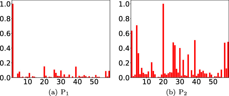
a, b Relevance scores for raw input features or parameters. x-axis: feature number, y-axis: relevance score. Here, P1: diabetes mellitus with complications, P2: essential hypertension
Fig. 13.
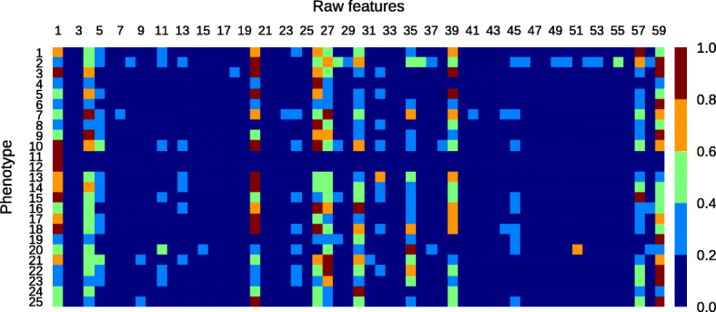
Feature relevance scores for 25 phenotypes using TimeNet-based transfer learning. Refer to Table 3 for the names of phenotypes and Table 4 for the names of raw features
Experimental Evaluation for Task Adaptation
Experimental Setup
We evaluate the HealthNet-based transfer learning approach on the same tasks as used in Section 8 with the following evaluation protocol as depicted in Fig. 9:
Fig. 9.
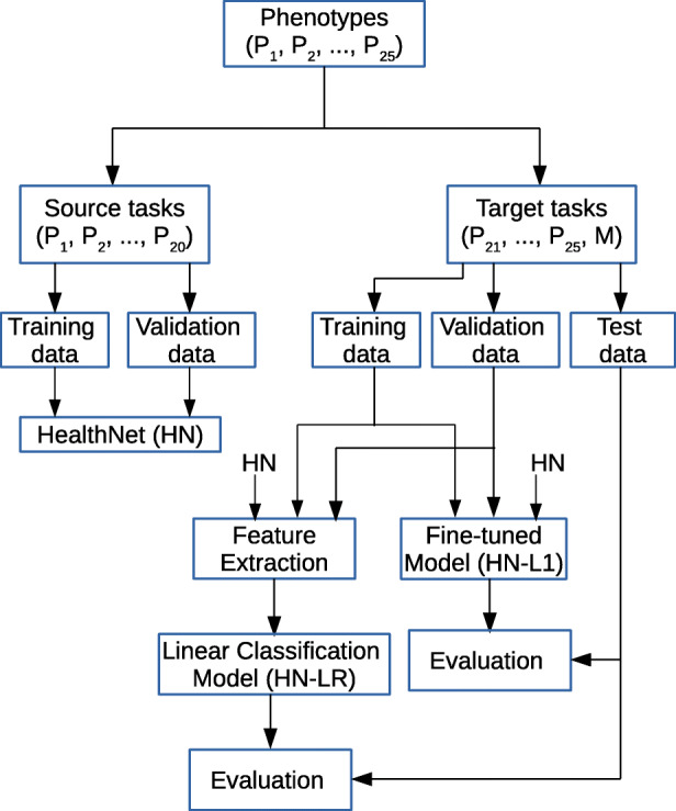
Evaluation protocol for task adaptation
Out of 25 phenotypes, we consider K = 20 phenotypes to obtain the pre-trained RNN which we refer to as HealthNet (HN) and test the transferability of the features from HN to remaining 5 phenotype classification tasks with varying labeled data sizes. Since more than one phenotype may be present in a patient at a time, we remove all patients with any of the 5 test phenotypes from the original train and validate sets (despite them having one of the 20 train phenotypes also) to avoid any information leakage. Except for this, note that the train, validate, and test splits remain the same as in[9]. We report average results in terms of weighted AUROC (as in [9]) on two random splits of 20 train (and validate) phenotypes and 5 test phenotypes, such that we have 10 test phenotypes (tested one-at-a-time). We also test the transferability of HN features to in-hospital mortality prediction task.
For each target task (i.e., 10 phenotypes and in-hospital mortality prediction task), we test the robustness of HN to labeled training data size. We use random stratified sub-sampling of the training and validation data to obtain reduced labeled training and validation sets. We consider the number of hidden layers L = 2, batch size of 128, regularization using dropout factor [26] of 0.3, and Adam optimizer [15] with initial learning rate 10− 4 for training RNNs. The number of hidden units h with minimum (3) on the validation set is chosen from {100,200,300,400}. Best HN model was obtained for h = 300 such that total number of features is m = 600. For fine-tuning of HN, we use the same parameters as used in training HN with regularization factor λ = 0.01 (4 and 5). For the linear classification model, the parameter λ is tuned on {0.1,1.0,…,104} (on a logarithmic scale) to minimize (6) on the validation set.
Results and Observations
We refer to the fine-tuned model using L1 regularizer as HN-L1, using L2 regularizer as HN-L2, without regularizer as HN-Tune, and LR model learned using HN features as HN-LR, and consider two baselines for comparison: (i) logistic regression (LR) using manually designed statistical features described in Section 8.1 and (ii) RNN classifier (RNN-C) with gated units as in LSTMs (or GRUs) obtained using training and validation data for the target task. To test the robustness of the models for small-labeled training sets, we consider subsets of training and validation datasets as explained in Section 9.1, while the test set remains the same. Further, we also evaluate the relevance of layer-wise features zτ, l from the L = 2 hidden layers of HealthNet. HN-LR-1 and HN-LR-2 refer to models trained using zτ,2 (the topmost hidden layer only) and zτ = [zτ,1, zτ,2] (from both hidden layers), respectively.
Comparing Variants of HealthNet-Based Transfer Learning Techniques
The results for phenotyping tasks in Fig. 10a suggest that (i) all the variants of HN-based transfer learning performs equally well on 100% training data; (ii) regularized fine-tuned models (HN-L1 and HN-L2) consistently outperform non-regularized fine-tuned model (HN-Tune) as training dataset is reduced. Importantly, as the size of labeled training set is reduced, non-regularized fine-tuned model degrades quickly as it is prone to overfitting due to a large number of trainable parameters. (iii) For medium-sized datasets (20% and 60% of original training data), the fine-tuned models HN-L1 and HN-L2 perform better than feature extraction based HN-LR models as well as the models without any regularization. However, for extremely large or small data sizes (5% and 100% cases), the difference is insignificant, thus indicating the expected trade-off between fine-tuning and feature extraction-based methods w.r.t. training data size: when labeled training data is small, fine-tuning all the parameters of a deep network may still be prone to some overfitting even after careful regularization.
Fig. 10.

a, b Classification performance comparison along with 95% confidence intervals for phenotyping task. Here, baseline models are LR and RNN-C, W-AUROC is weighted-AUROC over 10 phenotypes
Robustness of Transfer Learning Models Versus Models Trained From Scratch to Training Data Size
We compare the best fine-tuning based and feature extraction based variants, i.e., HN-L1 and HN-LR-2, with the LR and RNN-C models trained from scratch. As shown in Fig. 10b, we observe that:
(i) HN-L1, HN-LR-2, and RNN-C perform equally well when using 100% training data, and are better than LR. This implies that the transfer learning–based models are as effective as models trained specifically for the target task on large labeled datasets while reducing training efforts and automating feature extraction.
(ii) HN-L1 consistently outperforms RNN-C and LR models as training dataset is reduced. As the size of labeled training dataset reduces, though the performance of the model trained from scratch (RNN-C) as well as transfer learning models (HN-L1 and HN-LR-2) degrades, we observe that transfer learning based models degrade much more gracefully and perform significantly better than RNN-C for reduced data sizes (here, the 5% labeled data scenario). The performance gains from transfer learning are greater when the training set of the target task is small. Therefore, with transfer learning, fewer labeled instances are needed to achieve the same level of performance as model trained on target data alone.
(iii) As labeled training set is reduced, LR performs better than RNN-C confirming that deep networks are prone to overfitting on small datasets.
We also evaluate the transfer learning approach on in-hospital mortality task, and found transfer learning to be useful there as well. However, since the task is potentially unrelated to the phenotyping task, we do not observe significant improvements over the models trained from scratch. Refer to Fig. 12a in the Appendix for more details. From Fig. 12b, we interestingly observe that HN-LR-2 results are at least as good as RNN-C and LR on the seemingly unrelated task of mortality prediction, suggesting that the features learned are generic enough and transfer well.
Fig. 12.

a, b Classification performance comparison along with 95% confidence intervals for In-hospital mortality task. Here, baseline models are LR and RNN-C
Number of Relevant Features for a Task
We observe that only a small number of features are actually relevant for a target classification task out of large number of input features to LR models (714 for LR, 300 for HN-LR-1, and 600 for HN-LR-2). As shown in Table 2, > 95% of features have weight ≈ 0 (absolute value < 0.001) for HN-LR models corresponding to phenotyping tasks due to sparsity constraint (6), i.e., most features do not contribute to the classification decision. The weights of features that are non-zero for at least one of target tasks for HN-LR-1 are shown in Supplementary Material Fig. 14. We observe that, for example, for HN-LR-1 model, only 130 features (out of 300) are relevant across the 10 phenotype classification tasks and the mortality prediction task. This suggests that HN provides several generic features while LR learns to select the most relevant ones given a small-labeled dataset. Table 2 (and Fig. 14 in the Appendix) also suggests that HN-LR models use a larger number of features for mortality prediction task, possibly because concise features for mortality prediction are not available in the learned set of features as HN was pre-trained for phenotype identification tasks.
Table 2.
Fraction of features with weight ≈ 0. Here, the average and standard deviation over 10 phenotypes is reported for phenotyping task
| Series task | Series LR | Series HN-LR-1 | Series HN-LR-2 |
|---|---|---|---|
| Phenotyping | 0.902 ± 0.023 | 0.955 ± 0.020 | 0.974 ± 0.011 |
| In-hospital mortality | 0.917 | 0.787 | 0.867 |
Fig. 14.

Feature weights (absolute) for HN-LR-1. Here Pi (i = 1,…,10) denotes i-th phenotype identification task. x-axis: feature number, y-axis: task
Domain Adaptation Versus Task Adaptation
We study in what scenarios can domain adaptation be valuable compared with task adaptation and vice versa. To this effect, we consider a scenario where none or a very small number of source tasks from the healthcare domain are available for pre-training. When there is no source task from the healthcare domain for pre-training, the user has to resort to either training from scratch for the target task or use domain adaptation via TimeNet. However, when a small number (say, 2–3) of source tasks are available from the healthcare domain, it may be worth consider pre-training a healthcare domain-specific model rather than solely relying on TimeNet.
We evaluate on 5 binary classification target tasks, i.e., presence/absence of 5 phenotypes and report average results in Fig. 11. We use the same setup as in Sections 8 and 9 for domain and task adaptation, respectively. We vary the number of randomly chosen source tasks for task adaptation with K = {2,5,20} phenotypes out of the 20 remaining phenotypes (out of 25 tasks, 5 are used for testing) to obtain the pre-trained RNN, i.e., HealthNet (HN), and test the transferability of HN-L1 to 5 phenotypes with 20% of training data. We report the results using split K randomly selected train phenotypes out of 20 and 5 fixed test phenotypes, and report the average of three-run. For domain adaptation, we rely only on domain adaptation without using any of the K source tasks for pre-training.
Fig. 11.
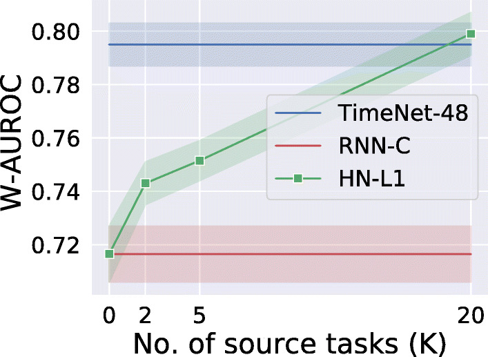
Classification performance comparison along with 95% confidence intervals. HealthNet-based transfer learning (HN-L1) versus TimeNet-based transfer learning (TimeNet-48). Here, W-AUROC is weighted-AUROC over 5 phenotype target tasks
Results and Observations
From Fig. 11, we observe that the performance of task adaptation approach HN-L1 degrades in comparison with domain adaptation approach (TimeNet-48) when the number of source tasks K available for training reduces. Further, TimeNet-48 and HN-L1 perform comparably when there is enough labeled data from a diverse set of tasks within the healthcare domain to allow for pre-training and leverage within-domain transfer. The advantage of TimeNet-like off-the-shelf generic models is evident as such models can be trained on publicly available time series data across domains in an unsupervised manner, and therefore, the performance of domain adaptation models is not very sensitive to the data in the healthcare domain. In other words, domain adaptation–based approaches are useful when there is not enough labeled data for the target task nor sufficient tasks in the target domain to pre-train a domain-specific model to leverage the benefits of transfer learning.
We also contrast the time taken to fine-tune TimeNet-based models and HealthNet-based models. Training and fine-tuning times are recorded on a 32GB RAM machine with Quad Core i7 2.7GHz processor. Training linear models (e.g., over TimeNet features) is fast, and it took around 10 min to obtain any of the target task-specific binary classifiers while tuning for α ∈ [10− 5 − 10− 3] (five equally spaced values). However, fine-tuning a deep learning model (e.g., HN) took around 45 min which is slower in comparison with TimeNet-based models but still faster than training a deep learning model (i.e., RNN-C) from scratch that took around 3 h for obtaining a final model while tuning for number of hidden units from {100, 200, 300, 400}.
Conclusion
Deep neural networks require heavy computational resources for training and are prone to overfitting. Scarce labeled training data, significant hyper-parameter tuning efforts, and scarce computational resources are often a bottleneck in adopting deep learning–based solutions to healthcare applications. In this work, we have proposed effective approaches for transfer learning in the healthcare domain by using deep recurrent neural networks (RNN). We considered two scenarios for transfer learning: (i) adapting a deep RNN-based universal time series feature extractor (TimeNet) to healthcare tasks and applications and (ii) adapting a deep RNN (HealthNet) pre-trained on healthcare tasks to a new related task. Our approach brings the advantage of deep learning such as automated feature extraction and ability to easily deal with variable length time series while still being simple to adapt to the target tasks. We have demonstrated that our transfer learning approaches can lead to significant gains in classification performance compared with traditional models using carefully designed statistical features or task-specific deep models in scarcely labeled training data scenarios. Further, leveraging pre-trained models ensures very little tuning effort, and therefore, fast adaptation. We also found that raw feature-wise handling of time series via TimeNet and subsequent linear classifier training can provide insights into the importance and relevance of a raw feature (physiological parameter) for a given task while still modeling the temporal aspect. This raw feature relevance scoring can help domain-experts gain at least a high-level insight into the working of otherwise opaque deep RNNs.
In future, evaluating a domain-specific TimeNet-like model for clinical time series (e.g., trained only on MIMIC-III database) will be interesting. Also, transferability and generalization capability of RNNs trained simultaneously on diverse tasks (such as length of stay, mortality prediction, and phenotyping [9, 32]) to new tasks is an interesting future direction.
Acknowledgments
We would like to thank the anonymous reviewers for their valuable comments that have helped to significantly enhance this paper.
Appendix: Multi-layered RNN with Gated Recurrent Units
A gated recurrent unit (GRU) [5] consists of an update gate and a reset gate that control the flow of information by manipulating the hidden state of the unit as in Equation (7).
In an RNN with L hidden layers, the reset gate is used to compute a proposed value for the hidden state at time t for the l-th hidden layer by using the hidden state and the hidden state of the units in the lower hidden layer at time t. The update gate decides as to what fractions of previous hidden state and proposed hidden state to use to obtain the updated hidden state at time t. In turn, the values of the reset gate and update gate themselves depend on the and
We use dropout variant for RNNs as proposed in [26] for regularization such that dropout is applied only to the non-recurrent connections, ensuring information flow across time steps.
The time series goes through the following transformations iteratively for t = 1 through T, where T is length of the time series:
| 7 |
where ⊙ is Hadamard product, [a, b] is concatenation of vectors a and b, D(⋅) is dropout operator that randomly sets the dimensions of its argument to zero with probability equal to dropout rate, and equals the input at time t. Wr, Wu, and Wp are weight matrices of appropriate dimensions s.t. , and are vectors in , where cl is the number of units in layer l. The sigmoid (σ) and tanh activation functions are applied element-wise.
Compliance with Ethical Standards
Conflict of Interest
The authors declare that they have no conflict of interest.
Footnotes
It is to be noted that we take TimeNet as an example to illustrate our proposed domain-adaptation approach, but the proposed approach is generic and can be used to adapt any universal time series feature extractor to healthcare domain.
Publisher’s Note
Springer Nature remains neutral with regard to jurisdictional claims in published maps and institutional affiliations.
Contributor Information
Priyanka Gupta, Email: priyanka.g35@tcs.com.
Pankaj Malhotra, Email: malhotra.pankaj@tcs.com.
Jyoti Narwariya, Email: jyoti.narwariya@tcs.com.
Lovekesh Vig, Email: lovekesh.vig@tcs.com.
Gautam Shroff, Email: gautam.shroff@tcs.com.
References
- 1.Bahdanau D, Cho K, Bengio Y (2014) Neural machine translation by jointly learning to align and translate. arXiv:14090473
- 2.Bengio Y (2012) Deep learning of representations for unsupervised and transfer learning. In: Proceedings of ICML workshop on unsupervised and transfer learning, pp 17–36
- 3.Che Z, Purushotham S, Cho K, Sontag D, Liu Y (2016) Recurrent neural networks for multivariate time series with missing values. arXiv:160601865 [DOI] [PMC free article] [PubMed]
- 4.Chen Y, Keogh E, Hu B, Begum N, et al. (2015) The ucr time series classification archive. www.cs.ucr.edu/eamonn/time_series_data/
- 5.Cho K, Van Merriënboer B, Gulcehre C, Bahdanau D, Bougares F, Schwenk H, Bengio Y (2014) Learning phrase representations using RNN encoder-decoder for statistical machine translation. arXiv:14061078
- 6.Choi E, Bahadori MT, Schuetz A, Stewart WF, Sun J (2016) Doctor ai: predicting clinical events via recurrent neural networks. In: Machine Learning for Healthcare Conference, pp 301–318 [PMC free article] [PubMed]
- 7.Gupta P, Malhotra P, Vig L, Shroff G (2018) Transfer learning for clinical time series analysis using recurrent neural networks [DOI] [PMC free article] [PubMed]
- 8.Gupta P, Malhotra P, Vig L, Shroff G (2018) Using features from pre-trained timenet for clinical predictions
- 9.Harutyunyan H, Khachatrian H, Kale DC, Galstyan A (2017) Multitask learning and benchmarking with clinical time series data. arXiv:170307771 [DOI] [PMC free article] [PubMed]
- 10.Harutyunyan H, Khachatrian H, Kale DC, Ver Steeg G, Galstyan A. Multitask learning and benchmarking with clinical time series data. Scientific Data. 2019;6(1):96. doi: 10.1038/s41597-019-0103-9. [DOI] [PMC free article] [PubMed] [Google Scholar]
- 11.Hermans M, Schrauwen B (2013) Training and analysing deep recurrent neural networks. In: Advances in neural information processing systems, pp 190–198
- 12.Hosmer DWJr, Lemeshow S, Sturdivant RX. Applied logistic regression, vol 398. Hoboken: Wiley; 2013. [Google Scholar]
- 13.Johnson AE, Pollard TJ, et al. Mimic-iii, a freely accessible critical care database. Scientific Data. 2016;3:160035. doi: 10.1038/sdata.2016.35. [DOI] [PMC free article] [PubMed] [Google Scholar]
- 14.Kashiparekh K, Narwariya J, Malhotra P, Vig L, Shroff G (2019) Convtimenet: a pre-trained deep convolutional neural network for time series classification. In: 2019 International joint conference on neural networks (IJCNN). IEEE
- 15.Kingma DP, Ba J (2014) Adam: a method for stochastic optimization. arXiv:14126980
- 16.Lee JY, Dernoncourt F, Szolovits P (2017) Transfer learning for named-entity recognition with neural networks. arXiv:170506273
- 17.Lipton ZC, Kale DC, Elkan C, Wetzel R (2015) Learning to diagnose with lstm recurrent neural networks. arXiv:151103677
- 18.Malhotra P, Vig L, Shroff G, Agarwal P (2015) Long short term memory networks for anomaly detection in time series. In: ESANN, 23rd European symposium on artificial neural networks, computational intelligence and machine learning, pp 89–94
- 19.Malhotra P, TV V, Vig L, Agarwal P, Shroff G (2017) TimeNet: pre-trained deep recurrent neural network for time series classification. In: 25th European symposium on artificial neural networks, computational intelligence and machine learning, pp 607–612
- 20.Micenková B, Dang XH, Assent I, Ng RT (2013) Explaining outliers by subspace separability. In: 2013 IEEE 13th international conference on data mining (ICDM). IEEE, pp 518–527
- 21.Miotto R, Li L, Kidd BA, Dudley JT. Deep patient: an unsupervised representation to predict the future of patients from the electronic health records. Scientific reports. 2016;6:26094. doi: 10.1038/srep26094. [DOI] [PMC free article] [PubMed] [Google Scholar]
- 22.Miotto R, Wang F, Wang S, Jiang X, Dudley JT (2017) Deep learning for healthcare: review, opportunities and challenges. Briefings in bioinformatics [DOI] [PMC free article] [PubMed]
- 23.Nguyen P, Tran T, Wickramasinghe N, Venkatesh S. Deepr: a convolutional net for medical records. IEEE J Biomed Health Info. 2017;21(1):22–30. doi: 10.1109/JBHI.2016.2633963. [DOI] [PubMed] [Google Scholar]
- 24.Pan SJ, Yang Q. A survey on transfer learning. IEEE Trans Knowl Data Eng. 2010;22(10):1345–1359. doi: 10.1109/TKDE.2009.191. [DOI] [Google Scholar]
- 25.Pascanu R, Mikolov T, Bengio Y (2013) On the difficulty of training recurrent neural networks. arXiv:12115063
- 26.Pham V, Bluche T, Kermorvant C, Louradour J (2014) Dropout improves recurrent neural networks for handwriting recognition. In: Frontiers in handwriting recognition (ICFHR). IEEE, pp 285–?290
- 27.Purushotham S, Meng C, Che Z, Liu Y (2017) Benchmark of deep learning models on large healthcare mimic datasets. arXiv:171008531 [DOI] [PubMed]
- 28.Rajkomar A, Oren E, Chen K, Dai AM, Hajaj N, Liu PJ, Liu X, Sun M, Sundberg P, Yee H, et al. (2018) Scalable and accurate deep learning for electronic health records. arXiv:180107860 [DOI] [PMC free article] [PubMed]
- 29.Ravì D, Wong C, Deligianni F, Berthelot M, Andreu-Perez J, Lo B, Yang GZ. Deep learning for health informatics. IEEE J Biomed Health Infor. 2017;21(1):4–21. doi: 10.1109/JBHI.2016.2636665. [DOI] [PubMed] [Google Scholar]
- 30.Serra J, Pascual S, Karatzoglou A (2018) Towards a universal neural network encoder for time series
- 31.Simonyan K, Zisserman A (2014) Very deep convolutional networks for large-scale image recognition. arXiv:14091556
- 32.Song H, Rajan D, Thiagarajan JJ, Spanias A (2017) Attend and diagnose: clinical time series analysis using attention models. arXiv:171103905
- 33.Sutskever I, Vinyals O, Le QV (2014) Sequence to sequence learning with neural networks. In: Advances in Neural Information Processing Systems, pp 3104–3112
- 34.Tibshirani R (1996) Regression shrinkage and selection via the lasso. Journal of the Royal Statistical Society Series B (Methodological): 267–288
- 35.Yosinski J, Clune J, Bengio Y, Lipson H (2014) How transferable are features in deep neural networks?. In: Advances in neural information processing systems, pp 3320–3328