Abstract
Covid-19, what a strange, unpredictable mutated virus. It has baffled many scientists, as no firm rule has yet been reached to predict the effect that the virus can inflict on people if they are infected with it. Recently, many researches have been introduced for diagnosing Covid-19; however, none of them pay attention to predict the effect of the virus on the person's body if the infection occurs but before the infection really takes place. Predicting the extent to which people will be affected if they are infected with the virus allows for some drastic precautions to be taken for those who will suffer from serious complications, while allowing some freedom for those who expect not to be affected badly. This paper introduces Covid-19 Prudential Expectation Strategy (CPES) as a new strategy for predicting the behavior of the person's body if he has been infected with Covid-19. The CPES composes of three phases called Outlier Rejection Phase (ORP), Feature Selection Phase (FSP), and Classification Phase (CP). For enhancing the classification accuracy in CP, CPES employs two proposed techniques for outlier rejection in ORP and feature selection in FSP, which are called Hybrid Outlier Rejection (HOR) method and Improved Binary Genetic Algorithm (IBGA) method respectively. In ORP, HOR rejects outliers in the training data using a hybrid method that combines standard division and Binary Gray Wolf Optimization (BGWO) method. On the other hand, in FSP, IBGA as a hybrid method selects the most useful features for the prediction process. IBGA includes Fisher Score (FScore) as a filter method to quickly select the features and BGA as a wrapper method to accurately select the features based on the average accuracy value from several classification models as a fitness function to guarantee the efficiency of the selected subset of features with any classifier. In CP, CPES has the ability to classify people based on their bodies’ reaction to Covid-19 infection, which is built upon a proposed Statistical Naïve Bayes (SNB) classifier after performing the previous two phases. CPES has been compared against recent related strategies in terms of accuracy, error, recall, precision, and run-time using Covid-19 dataset [1]. This dataset contains routine blood tests collected from people before and after their infection with covid-19 through a Web-based form created by us. CPES outperforms the competing methods in experimental results because it provides the best results with values of 0.87, 0.13, 0.84, and 0.79 for accuracy, error, precision, and recall.
Keywords: Covid-19, Prediction, Naïve Bayes, Prudential Expectation
1. Introduction
Covid-19, what a wondrous virus that has terrified many, as there is still no fixed base to predict the effects that the virus can cause to those who have been infected. At the beginning of the pandemic, some assumed that the elderly were at greater risk of death, and now we find that many of the elderly are recovering while death reaps many of the young [2,3]. Also, many healthy people, who were not suffering from any chronic diseases, were maliciously affected by the virus and many of them reached death, while others who have chronic diseases such as pressure, diabetes and heart have recovered from it. It is a mystery that needs everyone, not just medical professionals, to come together to find a solution. Covid-19, that spreads unexpectedly through droplets from an infected person's breath, cough, or sneeze [3,4]. The virus could be in the air or on surfaces that people may touch before touching their mouth, nose, or eyes. This gives the virus a passage to the mucous membranes in their throat. In a few days, patient's immune system may respond with several symptoms such as; a sore throat, diarrhea, a cough, shortness of breath, fever, chills, fatigue, body aches, headache, a runny nose, loss of taste and smell, nausea, or vomiting [2,5].
The ability to know the degree to which people bodies are affected if they are exposed to infection with Covid-19 before the actual infection occurs, beyond any doubt, allow some precautionary protocols to be taken according to the expected effect on the body [6,7]. Some people whose bodies are expected to bear the consequences of exposure to the virus may be allowed to mix with others and be in human gatherings. On the other hand, others who are expected to be badly affected by the consequences of the virus may be prevented from going out of the house even if they are not infected yet. This ability is called “Prudential expectation”. Generally, depending on doctors’ intuition and experience, clinical decisions have been made. This practice leads to high medical costs, errors, and unwanted biases which affects the quality of the provided service to patients [2,8]. All healthcare professionals usually store considerable amounts of patients’ data in the form of clinical databases. Analyzing these databases can certainly extract useful knowledge.
Depending on Data Mining (DM), a knowledge-rich environment based on the data hidden in the clinical databases can be generated. This can significantly enhance the accuracy of clinical decisions, promote the medical quality, and also save the waste of medical resources [2,9]. DM is an interesting area of Artificial Intelligence (AI) that refers to the knowledge discovery from real world datasets [6,10]. It is an interdisciplinary field that interacts with statistics, machine learning, pattern recognition, information retrieval, and databases [2,11]. DM is the process of exploring, modeling, and selecting large amounts of data to discover unknown relationships or complex patterns which introduce a useful and clear result to decision makers (e.g., doctors). Recently, data mining has been applied successfully in disease prediction and diagnosis [5,9].
Disease prediction aims to predict the risk factors associated with the major diseases, which helps health care professionals to identify patients at high risk of having a disease. Classification is the data mining technique that can be successfully applied for disease prediction [9,12]. In the last few years, different classification methods are used by researchers in the prediction of many diseases like stroke, diabetes, Human Immunodeficiency Virus (HIV), cancer, heart disease, and recently Covid-19 [13,14]. However, to the best of our knowledge, there is no prediction strategy for expecting the person's body reaction against having the disease till now. This expectation allows precautionary measures to be taken for those who are expected to suffer from serious complications that may cause disabilities or may lead to death if they are actually exposed to the disease. Hence, we call such process the “Prudential Expectation”, which is totally different from the classical disease prediction. Although both disease prediction and prudential expectation are performed before the infection and both rely on classification to perform the prediction, they have different targets. For a specific person, disease prediction aims to predict the risk of having the disease, while prudential expectation targets to predict the person's body reaction if he already infected by the disease.
The main contribution of this paper is to provide a Covid-19 Prudential Expectation Strategy (CPES). The aim of CPES is to predict the person's body reaction if he has infected by Covid-19. Hence, persons who will be badly influenced by the disease are subjected to prudential protocols. Others may have some freedom of being in human gatherings as it is predicted that their bodies can successfully resist the virus. CPES adopts a new strategy to predict the extent of the harm that may be caused to people if they are exposed to Covid-19 infection, and then apply the proper prudential protocols accordingly. CPES consists of three sequential phases, namely; ORP, FSP, and CP. The main objective of using ORP and FSP is to obtain pure data that is free from outliers and irrelevant features to enable the classification method in CP to provide fast and accurate results. Then, data will followed from ORP and FSP to the next phase called CP to correctly train the classification method and to enable it to provide the best classifications as possible. Outlier detection or anomaly detection is the process of determining data items with features that are very different from expectation. Outliers or anomalies should be rejected from the input training set. During ORP, a new technique has been introduced for rejecting outliers based on HOR method that combines the standard division and BGWO methods. While the standard division can speedily but not accurately eliminate outliers, the BGWO can accurately but not speedily reject outliers. Thus, the HOR is based on the implementation of standard division at first to quickly eliminate many outliers, and then the output of the standard division method is passed to BGWO to accurately eliminate outliers in the training data to enable the classification method in the CP to be learned correctly.
The main objective of FSP, on the other hand, is to select the best set of features that allow building a useful classification model. The aim of selecting the most significant features is not only to avoid overfitting but also to improve the model performance and to introduce faster and more cost-effective model. IBGA is a hybrid feature selection method applied in FSP to pick up the most informative features. IBGA combines filter and wrapper methods to utilize their benefits and provide fast and accurate subset of features as possible. IBGA consists of FScore as a filter method and BGA as a wrapper method. While FScore can quickly eliminate irrelevant features, BGA can accurately select the best subset of features depending on a new fitness function represents the average accuracy value from several classifiers to ensure the efficiency of the selected subset of features with any classifier. A new instance of NB classifier called SNB has been proposed to carry out the classification task in CP based on the filtered data from ORP and FSP. SNB is built upon the weighted NB algorithm, which estimates the relative importance of each feature, then assigns the appropriate weight to it. Hence, important features will have more weight than the less important or irrelevant ones. Since feature weighting uses continuous value, it impacts well in the final classification decision. CPES has been compared against recent techniques used for Covid-19 diagnoses. The efficiency and applicability of the proposed strategy has been proven in experimental results because it provides the maximum classification accuracy.
The remainder of the paper is organized as follows; Section 2 presents the problem definition and motivations. Section 3 discusses the previous effort about Covid-19 classification models. Section 4 introduces the proposed Covid-19 prudential expectation strategy. Next, the experimental setup and results have been provided in Section 5. Finally, the study and outlines the main directions for future work have been concluded in Section 6.
2. Problem definition and motivations
Despite the similarity in the physiological structure, humans differ from each other in the extent of response to diseases. Generally, human response to diseases is closely related to his level of immunity, however, there are many other factors that may significantly affect the extent of the human body's susceptibility to a particular disease compared to others. For example, at the beginning of the corona pandemic, it was believed that the extent to which a person was affected by Covid-19 is critically related to his age and his affliction with chronic diseases such as diabetes and pressure [2,9]. However, with the passage of time, it is noticed that old people who suffer from these diseases have been recovered with little effect. On the contrary, many healthy people of medium and low ages have affected by a huge impact, and sometimes it reached death [5,9].
Unfortunately, no test can distinguish live Covid-19 virus, accordingly, no test of infection is currently available. A person who tests positive with any kind of test may or may not be infectious. Moreover, several issues for Covid-19 are not clear yet such as; viral load, viral shedding, infection, infectiousness, and duration of infectiousness. On the other hand, the response of people's bodies and the extent of their susceptibility to disease are varying, despite the close proximity, whether in age or health status. Some people do not feel they have been infected with Covid-19, and the infection ended without the person feeling any symptoms or even they feel simple and normal symptoms. However, the status of other people, with similar conditions, may be developed into serious complications.
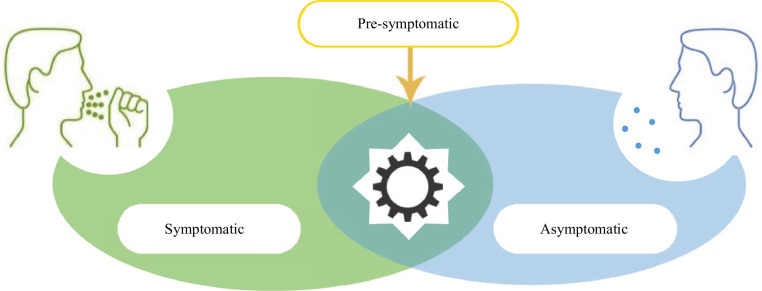
One of the strong reasons for Covid-19 quick spread is that some people who are infected with it have no symptoms and yet are contagious. It is strange that these people do not appear or feel ill, but they transmit the virus without realizing that. Spreading disease without illness appearance is called 'asymptomatic' (ASM) transmission. On the other hand, an infected person with disease signs is called a symptomatic (SYM) case. However, there exists another term that may cause confusion, which is; pre-symptomatic (PSYM). Although a PSYM case can be understood as simply someone who has not had any symptoms until now, PSYM can also mean ASM. Symptomatic, asymptomatic, and pre-symptomatic stages are illustrated in Fig. 1 .
Fig. 1.
Symptomatic, asymptomatic, and pre-symptomatic transmission.
As illustrated in Fig. 1, in the pre-symptomatic stage, many people are contagious, therefore, transmission of the virus is still possible although the disease is not externally manifested. This is why governments require entire families to isolate when one of their members gets sick. Hence, asymptomatic or pre-symptomatic cases have been called "silent diffusers". Hence, a critical task for limiting the fast spread of Covid-19 is to early identification of people who will be asymptomatic cases if they were infected by the virus before the actual infection takes place. A total of 634 people tested positive among 3,063 tests as at 20 February 2020 on board the Diamond Princess Cruise ship, Yokohama, Japan. Of the 634 confirmed cases, a total of 314 and 320 were reported to be symptomatic and asymptomatic respectively. The proportion of symptomatic and asymptomatic individuals during the period from13 to 20 February are illustrated in Fig. 2 , which indicates that there exists a clear evidence that a substantial fraction of Covid-19 infected individuals are asymptomatic [6,7]. The relatively high proportion of asymptomatic infections could have public health implications. Hence, more attention should be paid for those asymptomatic cases as they could be the hidden source of the virus infection spread.
Fig. 2.
Symptomatic versus asymptomatic cases on board the Diamond Princess Cruise ship, Yokohama, Japan, 2020.
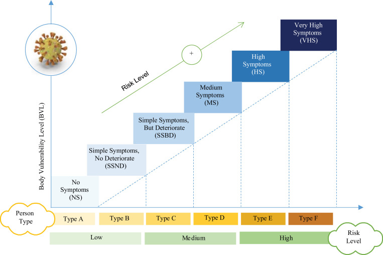
We are motivated to perform the work introduced in this paper because of the following reasons; (i) classifying people according to the extent to which their bodies will be affected by Covid-19 before the actual infection may limit the spread of corona disease and even eliminate it, (i) predicting how people's bodies will react if they are infected with corona can effectively help in taking appropriate precautionary measures according to the response of the human body, which can protect the individual from actual disease and (ii) the discovery of people who will not show symptoms of the disease or suffer from minor symptoms (e.g., asymptomatic cases) will have a great impact on limiting the spread of the disease. Those people who would not show symptoms act as time bombs as they continue interacting with healthy people and spreading the virus without realizing it. People classification based on their vulnerability level to Covid-19 in Fig. 3 . As illustrated in Fig. 3, based on the individual vulnerability level to Covid-19, people can be classified into six types (Type A→F). A person of ‘Type A’ will not show any symptoms if he infected by the virus, hence, he can be considered as asymptomatic case. ‘Type A’ will not be affected by the virus but he can spread it, so, he should be identified as he will be a silent spreader of the virus. On the other hand, the remaining types (e.g., Type B→F) are considered as symptomatic but with different vulnerability to the virus. To keep the society individuals safe, each type must be subjected to different treatments and rules as illustrated in Table 1 .
Fig. 3.
People classification based on their vulnerability level to Covid-19.
Table 1.
People classification based on their vulnerability level to Covid-19.
| Type | Description | Risk level | Treatment | Case |
| Type A |
|
|
|
Asymptomatic |
| Type B |
|
|
Symptomatic | |
| Type C |
|
|
|
|
| Type D |
|
|
||
| Type E |
|
|
|
|
The novelty of the work introduced in this paper is concentrated in the following points; (i) This paper is the first to introduce the problem of predicting how people's bodies will react if they are infected with corona, (ii) a new outlier rejection method is presented, which relies on standard division and Binary Gray Wolf Optimization (BGWO), (iii) based on an Improved Binary Genetic Algorithm (IBGA), a new feature selection method is introduced in this paper, which successfully classifies the features into three classes according to their effectiveness in the diagnose process, and finally, (iv) a new classification, which is based on a Statistical Naïve Bayes (SNB), that depends on the weighted NB algorithm classifier to give each feature a weight based on the calculation of feature convergence within the target classes and feature divergence among the target classes, has been introduced in this paper. Moreover, the effective coordination between the components of the prediction strategy proposed in this research has the greatest impact in providing impressive results.
3. Related work
This section will review the previous research efforts to classify Covid-19 patients. As introduced in [2], a new covid-19 detection strategy called Feature Correlated Naïve Bayes (FCNB) was implemented on the dataset that contains numerical laboratory tests findings for many cases of people. FCNB consists of two main stages called pre-processing stage and classification stage. In the first stage called pre-processing, three main phases called feature selection phase, feature clustering phase, and master feature weighting phase have been used. The feature selection phase was applied to select the informative features that effect on covid-19. Then, the feature clustering phase was used to put features into groups. At the end, the second stage called classification depended on a new algorithm called the weighted NB with several improvements. In experimental results, FCNB classification strategy could accurately detect Covid-19 patients.
In [5], Covid-19 Patients Detection Strategy (CPDS) as a new detection strategy was provided. The strategy depended on CT images for Covid-19 patients as well as non Covid-19 people in which it proposed two contributions. The first contribution was a new feature selection methodology, named; Hybrid Feature Selection Methodology (HFSM) that consists of two stages called fast selection stage and accurate selection stage. The main aim of HFSM was to select the most important features of Covid-19. On the other hand, the second contribution was an enhanced K-nearest neighbor classification model, which relies on determining the degree of both strength and closeness of each neighbor of the tested item then chooses only the qualified neighbors for classification. This strategy provided accuracy value equals to 0.96.
A new Hybrid Diagnosis Strategy (HDS) has been provided in [9]. HDS depended on a new methodology for ranking the elected features by projecting them into an introduced patient space. In fact, the rank of a feature was calculated based on two factors in which the first factor was feature weight while the second was its binding degree to its neighbors in the patient space. Then, the classification model was applied to accurately classify new patients to determine whether they are infected or not based on a hybrid classification model. This hybrid classification model included two main classifiers, which are; fuzzy inference engine and deep neural network. The proposed HDS provided values of recall, precision, accuracy, and F-measure equal 96.55%, 96.756%, 97.658%, and 96.615% respectively. Also, HDS introduced the lowest error value of 2.342%.
Distance Biased Naïve Bayes (DBNB) as a new strategy for diagnosing Covid-19 infected patients was proposed in [15]. It depends on the numerical laboratory tests findings for many cases of people. In fact, some of cases are infected with Covid-19 while some are not infected. This strategy depended on two contributions in which the first was Advanced Particle Swarm (APSO) as a hybrid feature selection methodology. APSO combines both filter and wrapper methods to select the most important features of Covid-19 for the next classification phase. On the other hand, the second contribution was a new classification methodology that combines both statistical and distance methods. The provided classification model contains two modules named weighted NB and distance reinforcement modules to overcome the issues of the traditional NB. According to the experimental results, DBNB outperformed the recent Covid-19 diagnose strategies in terms of accuracy, recall, precision, and F-measure.
In [16], convolutional neural network was applied to build the Deep Learning Model (DLM) to diagnose Coivd-19 patients based on various radiology domains. DLM consists of 27 layers which were validated on Computed Tomography (CT), X-ray, and Magnetic Resonance Imaging (MRI) datasets. The experimental results showed that the weighted average accuracies for the DLM according to CT, MRI, and X-ray are 85%, 86%, and 94% respectively. As presented in [17], a new Covid-19 detection model called Convolutional Neural Network-based Deep Learning (CNN-DL) was introduced to provide accurate diagnosis by using Chest X-Ray (CXR) images. CNN-DL model used the average of the parameters’ weights from many models fitted into a single model to extract features from images. Then, these extracted features were passed to a classification model to provide Covid-19 detection. According to the evaluation results, the CNN-DL was better than the competing methods with an accuracy of 95.49%.
As introduced in [18], a Hybrid Diagnosis Method (HDM) was provided to diagnose Covid-19 from CT images. The implementation of HDM based on many steps. Initially, extracting features from CT images was performed by using a Convolutional Neural Network (CNN) method, and then a tree Parzen estimator was applied to optimize the hyper parameters of the CNN. Additionally, a genetic algorithm was used to select the best subset of features, and at the end four different classification models were used to provide Covid-19 detection. The evaluation results showed the superiority of HDM over its competing methods with an accuracy of 0.997.
In [19], Aquila Optimizer (AO) that mimics the behavior of Aquila was introduced as a meta heuristic technique. Four methods have been used to represent the procedures of AO which are search space, exploring by contour flight with short glide attack, exploiting by low flight with slow descent attack, and swooping. To evaluate the performance of AO against other optimization techniques, many benchmark functions have been used. The evaluation results showed that AO outperformed other meta heuristic methods. As provided in [20], multilevel thresholding image segmentation issues could be solved by using an improved of the arithmetic optimization algorithm called DAOA that included the Differential Evolution technique with the Arithmetic Optimization Algorithm. The main objective of DAOA is to enhance the local search of the AOA and to construct equilibrium through the search techniques. The proposed DAOA outperformed other meta heuristic methods in the experimental results.
4. The proposed Covid-19 Prudential Expectation Strategy (CPES)
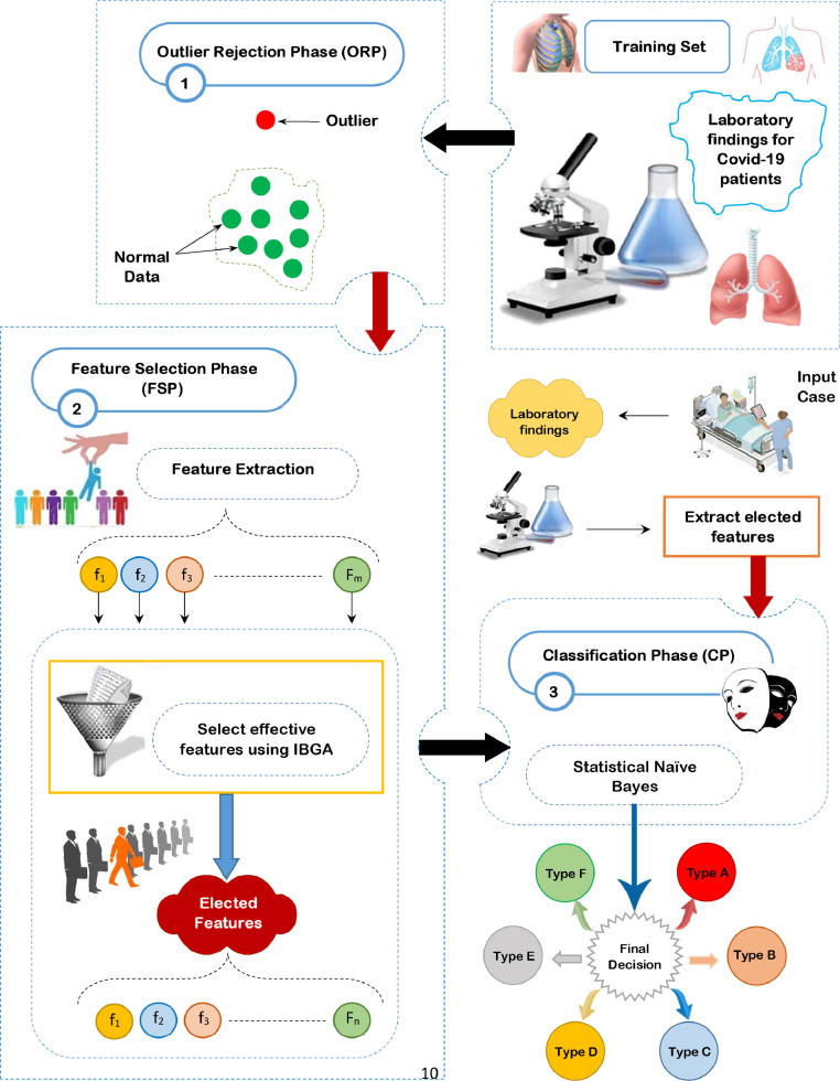
In this section, the proposed Covid-19 Prudential Expectation Strategy (CPES) will be discussed in details. CPES aims to classify people based on their bodies’ reaction to Covid-19 infection in a fast and accurate manner. CPES is a new strategy that predicts the extent of the harm that may be caused to people if they are exposed to Covid-19 infection and then apply the proper prudential protocols accordingly. In fact, CPES composes of three sequential phases, which are; ORP, FSP, and CP as shown in Fig. 4 . In ORP, HOR method will be provided in order to quickly and accurately reject outliers based on using the standard division as a fast outlier rejection method and BGWO as an accurate outlier rejection method based on the passed data from the standard division. FSP aims to select the most significant subset of features using IBGA that consists of FScore as a fast selection method and BGA as an accurate selection method based on the passed data from the FScore. BGA uses the average accuracy value from many different classifiers as a fitness function to determine the best chromosome that proves effective over several classifiers. Then, SNB will be used in the CP to perform the classification task based on the filtered data from ORP and FSP. In fact, SNB is built upon the weighted NB algorithm classifier that gives each feature a weight based on the calculation of feature convergence within the target classes and feature divergence among the target classes. The main objective of both phases called ORP and FSP is to provide a filtered dataset without outliers or irrelevant features to correctly learn the SNB classifier in the CP and give it the ability to provide fast and accurate classifications. These three phases will be depicted in details in the next sub-sections.
Fig. 4.
The proposed Covid-19 Prudential Expectation Strategy (CPES).
4.1. Outlier Rejection Phase (ORP)
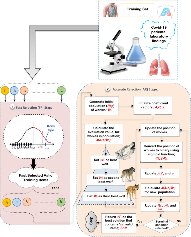
Outlier rejection is the process of finding data items that are completely different from expectation in a training dataset [10,11]. In this section, a Hybrid Outlier Rejection (HOR) method is provided as a simple but effective outlier rejection method to remove outlier items to enable the classification technique to perform its tasks quickly and accurately. The proposed HOR method mainly composes of two stages, called; Fast Rejection (FR) stage and Accurate Rejection (AR) stage as shown in Fig. 5 . In FR stage, standard division is used as a statistical-based method to quickly reject outliers from the training dataset as possible [21,22]. In AR stage, Binary Gray Wolf Optimization (BGWO) method is used as an optimization technique to accurately remove the rest of outliers in the training data to improve the performance of the classification model [23]. Although BGWO can accurately eliminate outliers in the training dataset, it suffers from the computational time. Thus, standard division method in FR stage preceded BGWO to quickly reject outliers before passing the medical dataset to BGWO method in AR stage. This process aims to reduce the BGWO execution time to provide a robust training dataset without outliers.
Fig. 5.
The sequential steps of HOR method.
Thus, the proposed HOR aims to quickly and accurately eliminate outlier items from the training dataset before starting to train classification technique. At the end, the optimal subset of training data is used to enable the classification model to perform its tasks well. Although BGWO has been widely applied in many works, it is used in this work as an outlier rejection method by using a reliable fitness function called Minimum Average Distance (MAD) that represents a distance-based outlier rejection method. Accordingly, AR stage uses a machine learning approach called BGWO based on MAD approach as a reliable fitness function. Hence, AR stage composes of a hybrid method that includes BGWO as a machine learning methodology [24,25] and MAD as an outlier rejection methodology [26]. Finally, HOR is a hybrid technique that consists of two main methods, called; (i) standard division as a statistical outlier rejection method and (ii) BGWO as a machine learning method that depends on distance-based method called MAD that represents a fitness function.
The sequential steps of HOR method using ‘nt’ training items are illustrated in Fig. 5. To implement HOR method, the medical dataset should be collected from hospitals. Then, the collected data should be passed to FR stage to implement standard division method to quickly reject outlier items from training dataset as possible (e.g., t “the number of valid items in the training dataset”), where, t<nt [21]. Then, the training dataset with ‘t’ valid items, which are passed from FR stage, are forwarded to AR stage to enable BGWO to quickly and accurately introduce a subset of valid training items without outliers. Secondly, iterations of BGWO will be performed until a termination condition is satisfied. Finally, the best search agent in the population called Alpha (α) introduces the most significant subset of valid training items that should be evaluated by using MAD method. MAD is used as a fitness function to evaluate the search agents in the population by calculating the average distance from each search agent in population and the center of every class category to give near-optimal solutions according to fitness function of an optimization issue.
Using BGWO as an outlier rejection method needs many basic steps as shown in Fig. 5. In AR stage, ‘nw’ search agents (wolves) are represented in Pop and then the evaluation (fitness) function of BGWO is applied to calculate the evaluation degree of each search agent Wi (subset of valid training items) based on a distance-based method called MAD. In fact, MAD method is implemented on every search agent Wi in population Pop where it represents the aggregated summation of the average distance at every class using (1).
| (1) |
where AvgC represents the average distance based on the valid training items which belong to class c in the ith wolf (search agent) where c = 1,2,…,cl. cl is the total number of class categories. The best search agent represents the search agent which provides the lowest fitness value (MAD) and vice versa. According to every search agent, the average distance AvgC of the valid items which belong to class c can be calculated by using (2).
| (2) |
where q’-z is the valid training items which in class c without z items as outliers and Eclid(Ih,Centerc) represents the distance between each training item Ih = [Ih(f1) Ih(f2) ... Ih(fm)] and its class center Centerc = [Centerc(f1) Centerc(f2) ... Centerc(fm)] using Euclidean Distance [11]. h is an index of the valid training item in the search agent which belongs to the class c and m is the number of features in the dataset. Consequently, if item Ih belongs to class c, then Eclid(Ih,Centerc) is given in (3).
| (3) |
where Ih(fj) is the value of item Ih at the feature fj. Centerc(fj) is the center value of class c at the feature fj, and m represents the features number. The formula of Centerc(fj) of class c at feature fj is given in (4).
| (4) |
where Ih(fj) represents the value of training item Ih that belongs to class c at the jth feature fj. q’ represents the training items (valid and invalid) in the dataset which are belonging to class c. BGWO algorithm searches for the best search agent (solution) with the goal of reducing MAD(Wi). Based on evaluation values for the search agents in Pop, the best three solutions; Wα, W β, and W δ will be assigned. Then, the other search agents in Pop including Omega (ω) will update their positions based on the position of Wα, W β, and W δ using (5) [23,24].
| (5) |
where ,, and are the positions of leaders Wα , W β, and W δ respectively according to the current search agent (Wi). In fact, the generated position value for each search agent Wi in Pop is a continuous value that cannot be directly used to reject outlier items and only provide valid items. Thus, the sigmoid function should be used as a transformation function to convert the continuous value to be a binary one. Consequently, every search agent's position; Wi = (Wi1, Wi2,…..,Wit) in Pop should be adjusted by applying the sigmoid function to identify new search agent's position based on binary values; Wbinary_i = (W1binary_i, W2binary_i,…..,Wtbinary_i) using (6) [23].
| (6) |
where Wkbinary_i (itr+1) represents the binary value of ith search agent at k th position in the next iteration itr+1. In other words, Wkbinary_i (itr+1) indicates to the value of kth training item in ith search agent; k = 1,2,3,…..,t. Additionally, rand(0,1) is a random value between [0,1] and sig(Wik) is the sigmoid transfer function that indicates the probability of kth bit in which it takes 0 or 1 value that is calculated by using (7) [23].
| (7) |
where e is the base of the natural logarithm. Based on the new position W kbinary_i (itr+1) of every search agent in Pop, every search agent is evaluated using the evaluation function in (1). Then, these calculations are continued until the number of generations is finished. Finally, the best solution Wα is the output and the algorithm terminates. All training items donated by zero (e.g, nr “the final number of valid items in the training dataset”) in this search agent represent the valid items which can be used to accurately learn the classification model, but the training items donated by one represent outliers which should be removed. After eliminating outlier items from training dataset, feature selection process should be implemented to select the most signification features on class category to enable the used classification model to provide fast and accurate results. Thus, feature selection process will be applied on dataset without outliers in the next sub-section.
4.2. Feature Selection Phase (FSP)
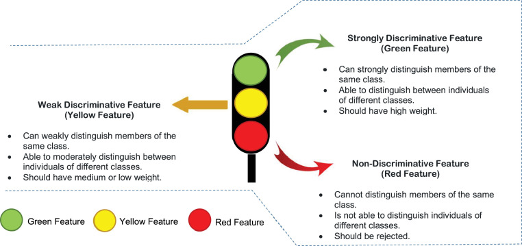
In fact, it is not only the outlier rejection process is the process that affects the efficiency of the classification model, but also feature selection process has a great effect on improving its efficiency by enabling it to give faster and more accurate classification [10,11]. The cause of overfitting problem may be the presence of irrelevant features in the dataset [2]. For accurate classification, the selected features should be able to distinguish members of the same class and also distinguish members of different classes. We call those features as discriminative. Based on our view, generally, features can be categorized into three different types, (i) Strongly Discriminative Feature (SDF) also called “Green Feature”, (ii) Weakly Discriminative Feature also called “Yellow Feature”, and (iii) Non-Discriminative Feature (NDF) also called “Red Feature” as shown in Fig. 6 . A discriminative feature (both strong and weak) should be used for the classification task. However, the non-discriminative ones should be eliminated through the FSP.
Fig. 6.
Different types of features.
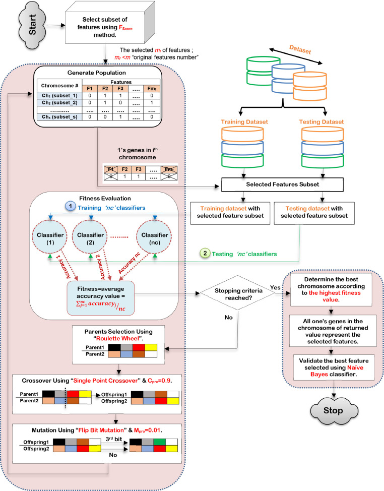
In this subsection, feature selection process will be implemented on dataset during this phase to select the informative features which have the best effect on the used classifier, which represents; Green Feature and Yellow Feature types. FSP tends to accurately select the most significant subset of features using a hybrid feature selection technique called Improved Binary Genetic Algorithm (IBGA). IBGA comprises of both filter and wrapper selection methods which are FScore and BGA respectively. The main objective of IBGA is to improve the performance of BGA as it consumes a long execution time; therefore, FScore is put in the foreground before using BGA to quickly remove many useless features to reduce the execution time of BGA implementation. To implement IBGA method, FScore is initially applied to quickly remove most of the useless features in the dataset [10]. Then, BGA is executed based on the passed data from FScore using a better fitness function to evaluate every chromosome in the population. The fitness function used in IBGA is the average accuracy value from several classification models trained on the same data to generalize the evaluation of chromosomes in the population. In other words, the calculation of fitness values for chromosomes in IBGA depends on several classifiers rather than using only a particular classifier to ensure the generality of the feature selection. Hence, the subset of features which have a significant and effective effect on most classification methods and not for a particular one classifier will be selected to ensure the effectiveness of the selected features on any classification model. To implement IBGA methods, many sequential steps will be followed as shown in Fig. 7 .
Fig. 7.
The sequential steps of IBGA.
According to Fig. 7, after implementing FScore, IBGA begins with a population that contains many chromosomes in which each chromosome consists of a series of genes in form of bits [27,28]. The length of each chromosome is the number of features in dataset with binary values (0 or 1) where ‘1’ in the jth position in the chromosome means that the jth feature is selected and ‘0’ means that the jth feature is removed. After generating a population of ‘s’ chromosomes that represent ‘m’ features in binary space, fitness evaluation will be calculated to measure the fitness degree of each chromosome in population (subset of input features). The fitness (evaluation) function is the average accuracy value from ‘nc’ classifiers to ensure that the selected subset of features is the best subset that can improve the performance of any classifier to provide fast and accurate classification. The fitness function according to ‘nc’ classifiers can be calculated for ith chromosome (Chi) by using (8).
| (8) |
where Fit(Chi) is the fitness evaluation value for ith chromosome, Accuracyj(Chi) is the accuracy value of jth classifier according to the selected features in ith chromosome, and nc is the number of classifiers used to evaluate the selected features in each chromosome. To clarify the idea, assume that there are two chromosomes in population; s = 2 and three classifiers; nc = 3, used to evaluate the selected features in every chromosome as presented in Table 2 .
Table 2.
Determine the best chromosome based on both every classifier and average accuracy.
| Classifier # | Accuracy of every chromosome |
The best chromosome | |
| Ch1 | Ch2 | ||
| C1 = NB | 0.75 | 0.7 | Ch1 |
| C2 = KNN | 0.9 | 0.7 | Ch1 |
| C3 = SVM | 0.8 | 0.9 | Ch2 |
| Average accuracy | 0.816 | 0.767 | Ch1 |
According to Table 2, it is assumed that the used classifiers are Naïve Bayes (NB) [29,30,31], K-Nearest Neighbors (KNN) [5], and Support Vector Machine (SVM) [11]. Based on their accuracy values for chromosomes, it is noted that NB and KNN proven that the first chromosome (Ch1) is better than the second one. On the other hand, SVM proven that the second chromosome (Ch2) is better than the first one. Finally, the best chromosome is the first one based on the average accuracy value. Accordingly, depending on single classifier to determine the fitness evaluation for chromosomes cannot generally provide the optimal subset of features that can adaptive with any used classifier. For this reason, the fitness function in this work is based on using the average accuracy value to provide a global solution that includes only Green Feature and Yellow Feature without Red Feature.
After evaluating all chromosomes in the population, the termination condition should be checked to determine if it is satisfied or not. In the case if the termination condition is not satisfied, the three biologically inspired BGA operators, which are; selection, crossover, and mutation will be continued to produce a new generation of chromosomes. While selection process attempts to select good chromosome, crossover process combines good chromosomes to produce better offspring's in the new generation. Chromosome can be locally changed to create better chromosome by performing mutation. In this work, the selection process will be performed using roulette wheel method based on different probability of selection (Spro) according to every chromosome in the population, the crossover process will be performed by using single point crossover based on probability of crossover (Cpro), and a flip bit mutation method will be used to perform the mutation process based on probability of mutation (Mpro) [2,11]. In fact, the probabilities values of Spro, Cpro and Mpro are random values between 0 and 1 (0 ≤ Spro, Cpro and Mpro ≤ 1). In general, crossover operation is preferred over mutation operation, thus, Cpro usually equals 0.9 while Mpro equals 0.01to enable BGA to perform its tasks well. On the other hand, if the termination condition is satisfied, the algorithm will be terminated and the best subset of features is represented in the chromosome that provides the highest fitness value. After eliminating outlier items from training dataset and then selecting the most significant subset of features in the used dataset, classification model should be learned to provide fast and accurate results. Thus, classification process will be applied on dataset without outliers and irrelevant features in the next sub-section.
4.3. Classification Phase (CP)
Despite its simplicity, NB classifier is one of the powerful classification techniques. Due to its easiness, along with its good performance, NB is widely used to address classification problems in several real-world applications [28,32]. NB has been chosen to be implemented in CP for the following reasons; (i) it can provide fast predictions rather than other classification algorithms because the training time has an order O(N) with the dataset, (ii) NB can be easily trained with small amount of input training dataset and it can be used also for large datasets as well, (iii) NB is easy to be implemented with the ability of real-time training for new items, (iv) it has no required adjusting parameter or domain knowledge, (v) NB is less sensitive to missing data, (vi) it has high capability to handle the noise in the dataset, (vii) NB is Incremental learning algorithm because NB functions work from approximation of low-order probabilities which are extracted from the training data [33,34,35]. Hence, these can be quickly updated as new training data are obtained, (ix) it is sufficient for real-time applications such as diseases diagnoses because it relies on a set of pre-computed probabilities that make the classification done in a very short time [29,33].
However, NB assumes that all features are independent, which is rarely happening in real life. This assumption limits the applicability of this algorithm in real-world use cases. In order to alleviate such independence assumption, a mass of feature weighting approaches have been proposed. However, almost all of these approaches do not guarantee high performance. Accordingly, there is a critical need for more fine-grained feature weighting technique. To our best of knowledge, up to the present, there is little work on it. Through this section, a new feature weighting paradigm will be introduced to build a new instance of the classical NB algorithm, which is called Statistical Naïve Bayes (SNB). Generally, the success of the classification is built upon the accurate selection of discriminative features. Hence, a weight can be given to each feature to measure its ability for discrimination, which can be called the feature weight [31]. In the proposed SNB, the weight of each feature is calculated according to how close the value of that feature is in the elements of the same class and how far apart the values of that feature are between the items of the different classes. To accomplish such aim, two important values should be calculated for estimating the weight of a specific feature, which are; (i) the degree of convergence of the feature values within the target classes and (ii) the degree of divergence of the feature values among the target classes. More details about those two issues are explained in the next sub-sections.
4.3.1. Estimating Feature Convergence Within the Target Classes
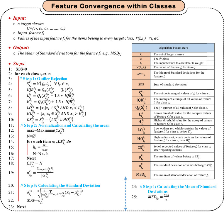
Generally, members (items) within the same target class should be similar. The similarity is measured by the degree of closeness of values of the considered feature values among the class members. Hence, for a specific feature fx, its values should be converged among the members of the same class. Estimating the convergence of a specific feature fx can be accomplished through the four sequential steps, which are; (i) rejecting outlier values of fx for each target class, (ii) calculating the mean for the values of the considered feature fx for each target class after rejecting outliers, (iii) calculating the standard deviation for the values of the considered feature fx for each target class after rejecting outliers, and (iv) calculating the Mean of Standard Deviation (MSD) for the feature fx. Finally, the more, the less the weight of fx. As illustrated in Algorithm 1, estimating the feature convergence within the target class can be achieved by calculating . To accomplish such aim, the first step is to reject outlier values for the feature fx within each of the considered target classes. An outlier is a data point that fall outside the overall pattern in a distribution. Low outliers are below Q1-1.5 × IQR and high outliers are above Q3+1.5 × IQR, where Q 1 is the first quartile, which represents a quarter of the way through the list of all data and Q 3 is the third quartile, which represents three-quarters of the way through the list of all data.
Algorithm 1.
Feature Convergence within Classes Algorithm.
Generally, IQR is calculated in much the same way as the range. To find IQR, subtract the first quartile from the third quartile as; IQR = Q 3 – Q 1. It can be used to detect outliers using the following steps; (i) Calculate the interquartile range for the data, (ii) Multiply the interquartile range (IQR) by 1.5 (a constant used to discern outliers), (iii) Find H = Q3+1.5 x (IQR). Hence, any data point greater than H is a suspected high outlier, and (vi) Find L = Q1- 1.5 x (IQR). Hence, any data point less than L is a suspected low outlier. After rejecting outlier data point, the next step is to normalize moderate (accepted) values, then calculate the mean (μ) of the considered feature values for each target class using (9).
| (9) |
where is the mean of the considered values of feature fx assuming ci as the target class and xi is the index that refers to each value of feature fx. is the set of the considered values of feature fx assuming ci as the target class. Then, the standard deviation for all values in ∀ ci ∈C is calculated using (10).
| (10) |
The mean of standard deviations for the feature fx, which indicates the degree of convergence of fx values within each of the target classes can be calculated using (11).
| (11) |
where is the mean of standard deviations of the feature fx, is the standard deviation of fx considered values after rejecting outliers considering ci as the target class, C is the set of target classes, and n is the number of target classes. Generally, is an indication for the degree of convergence of the feature fx within the target classes. Hence, the more the value of , the less the weight of the feature fx. The next step is to calculate the inverse of , which is denoted as; . So, the more the , the more the weight of fx. can be calculated using (12).
| (12) |
Finally, , where F is the set of the considered features, should be normalized to be in the range from 0→1. The result will be . Calculating can be done using (13).
| (13) |
where is the value to be normalized, is the maximum un-normalized value of IMSD considering all the elected features, and is the maximum target normalized value. Since the normalized range is assumed to be 0→1, then , and accordingly, can be expressed by (14).
| (14) |
4.3.2. Estimating Feature Divergence Among the Target Classes
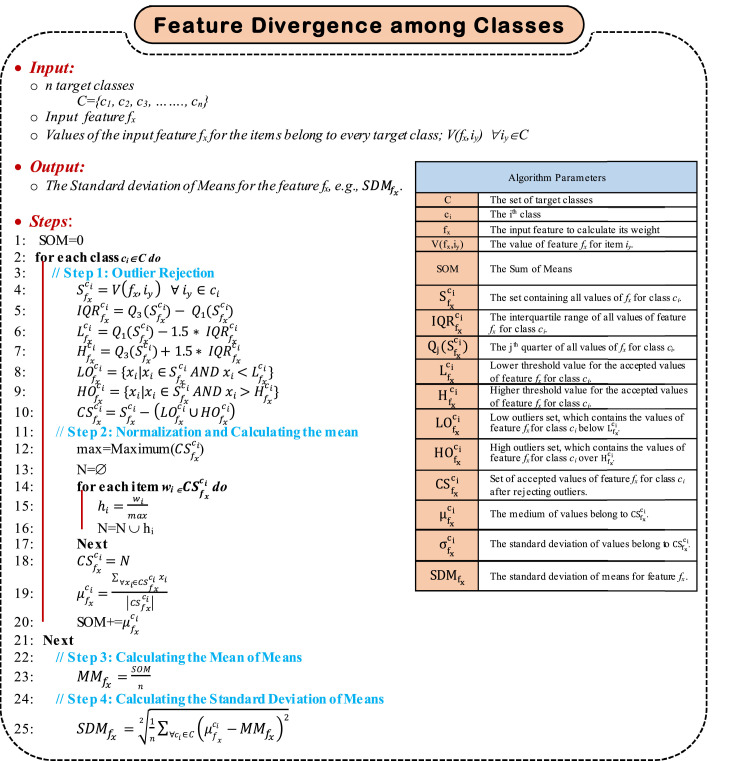
In fact, the discriminative features should be able to distinguish elements belonging to different target classes. To measure such ability, considering the feature fx, the feature divergence among the target classes is calculated. Then, the more feature divergence, the more feature discrimination ability, and accordingly, the more the feature weight. Estimating fx divergence among the target classes can be achieved by calculating the Standard Deviation of Means for fx, which is denoted as; . To accomplish such aim, the first step is to reject outlier values for the feature fx within each of the considered target classes using the interquartile range (IQR). After rejecting outliers, the next step is to normalize moderate (accepted) values, then calculate the mean (μ) of the considered feature values for each target class (e.g., ∀ ci ∈C) using (18). Then, the Mean of Means for fx, denoted as; , is calculated using (15).
| (15) |
where n is the number of target classes, is the mean of the considered feature values for each target class, and ci is the target class. Then, the Standard Deviation of Means for fx, denoted as; , can be calculated using (16).
| (16) |
where C is the set of target classes, n is the number of target classes, and the mean of means for fx, and is the mean of the accepted values of fx for the items belong to class ci. It can be concluded that; is an indication for the degree of divergence of the feature fx among the target classes. Hence, the more the value of , the more the weight of the feature fx. Finally, , where F is the set of the considered features, should be normalized to be in the range from 0→1. The result will be . Calculating can be done using (17).
| (17) |
where is the value to be normalized, is the maximum un-normalized value of SDM considering all the elected features, and is the maximum target normalized value. Since the normalized range is assumed to be 0→1, then , and accordingly, can be expressed by (18). The steps of feature divergence among classes algorithm is provided in Algorithm 2.
| (18) |
Algorithm 2.
Feature Divergence among Classes Algorithm.
4.3.3. ulating the Total Feature Weight
There are two basic factors that can be applied to calculate the total feature weight, called; (i) the feature convergence within the target classes that can be expressed by and (ii) the feature divergence among the target classes that can be expressed by . As shown before, the more and, the more the feature weight, hence;
and
Then, the weight of attribute (or feature) fx can be measured by (19).
| (19) |
here is the weight of the feature fx, is the normalized inverse mean of standard deviations for the feature fx, is the normalized standard deviation of means for the feature fx, and δδ and ββ are equation constants. Both values and range from 0→1. should be also ranges from 0→1, hence, it can be concluded that δδ+ββ = 1. The challenge now is to estimate the proper values of ββ and δδ to achieve the maximum classification accuracy. The procedure used for estimating δδ and ββ is depicted in Algorithm 3.
Algorithm 3.
(a) Estimating δδ and ββ graphically (b) Estimating the optimal values of δδ and ββ algorithm.
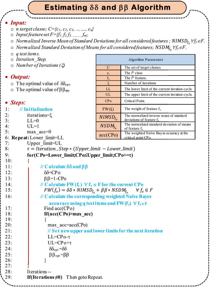
As depicted in Algorithm 3, it is needed to search for the best values of δδ and ββ, which introduce the highest accuracy of the classification method. To accomplish such aim, a CPo is used to tune the values of δδ and ββ looking for the maximum accuracy. As illustrated in Algorithm 3, two variables, namely; Upper_limit and Lower _limit are used to set the searchable range of CPo. Initially, setting Upper_limit and Lower _limit to 1 and 0 respectively results in a searchable range of CPo to be 0→1. An iteration step is set, which is used to calculate the gradual change in CPo, denoted as; τ. As CPo is updated, the corresponding classification accuracy is calculated. Once CPo reaches 1, the first iteration is then finished. A new iteration will immediately be started with a new searchable range for CPo. The new searchable range is a neighborhood around the value of CPo which produces the maximum classification accuracy in the previous iteration. The neighborhood width is assumed to be 2*τ. Such procedure continues based on a pre-defined number of iterations (e.g., ξ), expressed by the variable iterations in Algorithm 3. Finally, δδopt and ββopt are those values that introduce the maximum classification accuracy through all iterations. It will be easy now to calculate the feature weight using (19).
5. Experimental Results
In this section, the evaluation of the Covid-19 Prudential Expectation Strategy (CPES) is investigated. CPES consists of three phases, called; (i) Outlier Rejection Phase (ORP), (ii) Feature Selection Phase (FSP), and (iii) Classification Phase (CP). During ORP, a new technique called Hybrid Outlier Rejection (HOR) that combines both standard division and Binary Gray Wolf Optimization (BGWO) will be implemented to reject outliers in the training data. Then, Improved Binary Genetic Algorithm (IBGA) will be implemented in FSP to select the most important features for enhancing the performance of classification model. IBGA is a hybrid selection method that consists of a filter selection method called Fisher Score (FScore) and a wrapper selection method called Binary Genetic Algorithm (BGA). Finally, a new instance of NB classifier called SNB will be implemented in CP to quickly and accurately classify people based on their bodies’ reaction to Covid-19 infection. Two main scenarios for the implementation of the CPES will be pursued. According to the first scenario, the IBGA as a hybrid feature selection method will be tested against other modern selection methods using NB classifier as a standard classification method [29,30,31]. Then, the complete strategy called CPES will be tested against other modern diagnostic strategies. Our implementation depends on Covid-19 dataset [1]. Covid-19 dataset is divided into training set used to train the classification method and testing set used to measure the performance of the model. Accuracy, error, precision, and recall will be used to evaluate the following experiments based on the confusion matrix [2,11]. Additionally, the execution time (Run time) will be measured to calculate the speed of strategy execution. The corresponding used values of the applied tunable parameters are presented in Table 3 .
Table 3.
The corresponding used values of the applied tunable parameters.
| Parameter | Description | Applied value |
| Spro | Probability of selection | Random (0 ≤ Spro ≤ 1) |
| Cpro | Probability of Crossover | Random (0 ≤ Cpro ≤ 1) |
| Mpro | Probability of Mutation | Random (0 ≤ Mpro ≤ 1) |
| r1 and r2 | Two independent random numbers | Random (0 ≤ r1,r2 ≤ 1) |
| a | Linearly decrease | [2,0] |
| Max_iter_BGA | The maximum number of iterations for GA | 100 |
| Max_iter_BGWO | The maximum number of iterations for GWO | 100 |
5.1. Dataset Description
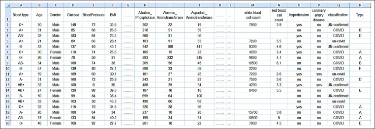
Nowadays, finding a research dataset to be used for Covid-19 disease researches represents a main challenge because this disease is a quite newly emerged type of coronaviruses. For overcoming this challenge, we create a Web-based form to collect routine blood tests from people before and after their infection with covid-19. This form is affiliated to artificial intelligence lab in Nile Higher Institute for Engineering and technology where the dataset is available at. [1]. The dataset contains 50 features extracted from numerical laboratory tests as described in Table 4 (a-c). In fact, the features have been reduced to be 37 features after implementing IBGA. The total number of people registered on the form until now is 2215 in which the number of infected people is 1389, 430 of them are un-covid-19 people, and 396 are unconfirmed cases as described in Table 5 . Actually, the dataset has been split into training dataset and testing dataset where the training dataset consists of 973 patients and the testing dataset consists of 416 patients. Based on the individual vulnerability level to Covid-19, patients in the dataset can be categorized into six types (Type A→F). Fig. 8 shows a snapshot from the Covid-19 dataset.
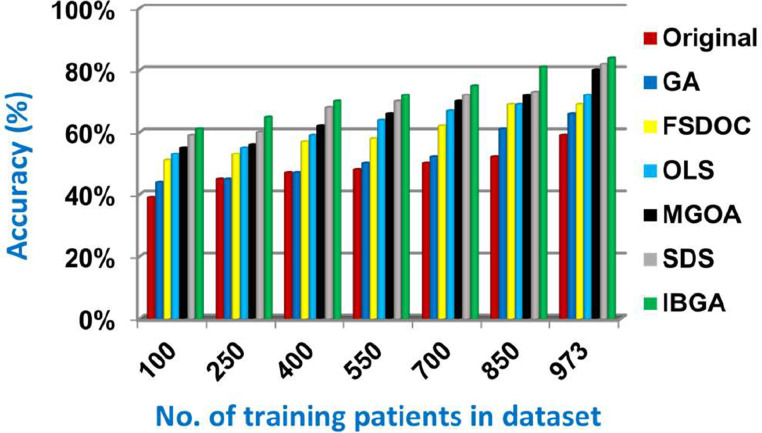
Fig. 9.
Accuracy of several feature selection methods.
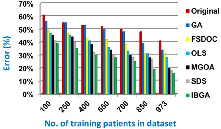
Fig. 10.
Error of several feature selection methods.
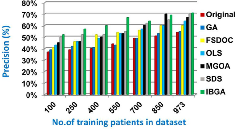
Fig. 11.
Precision of several feature selection methods.
Table 4.
Descriptions about the features of Covid-19.
| (a) | ||
| Feature | Description | Selected Feature |
| Age | Age of the patient. | Yes |
| Gender | Male / Female. | No |
| Glucose | Glucose represents the main type of sugar found in the blood. | Yes |
| Blood type | Determine the type of the blood. | Yes |
| Blood Pressure | It is the pressure of the blood on the walls of the arteries. | Yes |
| Body Mass Index (BMI) | BMI is a measure that indicates to total body fat. It is used to measure whether a person is at a healthy weight. | Yes |
| Diabetes Pedigree Function | A function that scores the likelihood of diabetes based on family history. | No |
| Total_Bilirubin | It is a measure of liver function in which it measures the amount of a substance called bilirubin in the blood. | Yes |
| Direct_Bilirubin | It is a measure of the amount of conjugated bilirubin in which it looks for bilirubin in the urine or blood. | Yes |
| Alkaline_ Phosphotase | It is a measure of the amount of alkaline phosphotase in your blood in which Alkaline_ Phosphotase is an enzyme found throughout the body. Actually, it is mostly found in the liver, digestive system, kidneys, and bones. | Yes |
| Alamine_ Aminotransferase (ALT) | ALT is an enzyme that is normally found in the cells of the liver and kidney. When ALT levels in blood are high that means a liver is damaged. | Yes |
| Aspartate_ Aminotransferase (AST) | AST is an enzyme that is normally found in liver and heart. When AST levels in blood are high that indicates liver diseases and heart problems or pancreatitis. | Yes |
| Total_ Protiens | It is a measure of the amount of protein in your blood. When total protein level is high that indicates dehydration or a certain type of cancer. | No |
| Albumin | It is protein that is made by liver in which it is a test that measures of the amount of albumin in the blood. | Yes |
| Globulin_Ratio | It is a ratio of albumin to globulin in blood plasma. | Yes |
| Red blood count | It is a blood test that is used to measure how many red blood cells that contain haemoglobin, which carries oxygen throughout the body. | Yes |
| Pus Cell | It is a white blood cell (as a neutrophil) that is found in pus. | No |
| Bacteria | Bacteria are used to help diagnose certain types of infections in which their organisms not visible with the naked eye. | Yes |
| Blood urea test | It measures the amount of nitrogen in the blood. When your blood urea level rises, this means that your kidneys cannot remove urea from the blood normally. | Yes |
| (b) | ||
| Feature | Description | Selected Feature |
| Serum creatinine | It indicates kidney health in which it is an easily measured by product of muscle metabolism. | Yes |
| Sodium | A sodium is a part of an electrolyte panel that is used as a blood test to measure the amount of sodium in the blood. | Yes |
| Potassium | A potassium is a part of an electrolyte that is used as a blood test to measure the amount of potassium in the blood. | Yes |
| Haemoglobin | It is a blood test that is used to measure the amount of haemoglobin in the blood in which it carries oxygen to organs and tissues in the body and also transfer carbon dioxide from organs and tissues to lungs. | Yes |
| Packed cell volume | It's a test used to determine whether a patient has polycythaemia, dehydration, or anaemia. It's usually part of a whole blood count test. | No |
| White blood cell count |
The immune system is made up of white blood cells. They aid in the battle against infections and other disorders. | Yes |
| Hypertension | It is a disorder in which the blood arteries have a consistently elevated pressure. Hypertension is a significant medical condition that can put your heart, brain, kidneys, and other organs at risk. | Yes |
| Pedal edema | The medical term for swelling is edoema. Injuries and inflammation cause body parts to swell. edoema might affect a small portion of the body or the full body. | No |
| Resting electrocardiographic results | It's a medical test that measures the electrical activity generated by the heart while it contracts to diagnose heart abnormalities. | Yes |
| Anemia | Anemia is a condition in which the number of red blood cells or haemoglobin is lower than normal. | Yes |
| Diabetes mellitus | Diabetes mellitus is a disorder in which the body's ability to form of sugar is impaired. | Yes |
| Coronary artery disease | The coronary arteries supply your heart with blood, oxygen, and nourishment. Coronary artery disease develops when your heart's primary blood arteries become damaged or diseased. | Yes |
| Appetite | The appetite test is used to determine the appetite of a person. | No |
| Maximum heart rate achieved |
The number of contractions (beats) of the heart per minute is used to determine the heart rate (bpm). | Yes |
| Exercise induced angina | Angina is chest pain that occurs as a result of exercise, stress, or other factors that cause the heart to pump harder. It's a symptom of coronary artery disease that's very frequent. | Yes |
| Atherosclerosis | Arteriosclerosis is a condition in which the arteries that carry oxygen and nutrients from your heart to the rest of your body thicken and stiffen, reducing blood flow to your organs and tissues. | Yes |
| D-Dimer | A D-dimer test examines the presence of D-dimer in the blood. When a blood clot dissolves in your body, a protein fragment called a D-dimer is formed. | Yes |
| C-Reactive Protein (CRP) | CRP is a protein made by the liver, and the CRP test is used to discover or monitor inflammatory diseases. | Yes |
| Lactate Dehydrogenase (LDH) | The LDH test is performed to detect any tissue damage. | Yes |
| Troponin | Troponins are a family of proteins that govern muscular contraction in skeletal and cardiac muscle fibres. Troponin tests detect heart damage by measuring the quantity of cardiac-specific troponin in the blood. | Yes |
| (c) | ||
| Feature | Description | Selected Feature |
| Platelets Count (PC) | The platelet count (PC) is a blood test which measures the average amount of platelets in a person's blood. Platelets aid in the healing of wounds and the prevention of excessive bleeding in the bloodstream. | Yes |
| Neutrophils Count (NC) | Neutrophils are a type of WBC that form (50-75%) of the total. NC gives critical information regarding the patient's health status. | Yes |
| Lymphocytes Count (LC) | The lymphocyte count, which is a component of WBC, is determined by LC test. | Yes |
| Monocytes count | The quantity of monocytes circulating in the blood is measured by the monocytes count test. | No |
| Eosinophil | Eosinophil is a type of white blood cell that helps the immune system combat disease by preventing infections and increasing inflammation. | No |
| Basophils | Basophils are bone marrow-derived white blood cells that aid in the proper functioning of the immune system. | No |
| Gamma-Glutamyl Transpeptidas (GGT) |
GGT is an ubiquitous enzyme found throughout the body. GGT levels in the blood can indicate bile duct damage or liver disease; a GGT test can determine the quantity of GGT in the blood. | No |
| Chest pain type | The discomfort in the chest or presence of abnormal pain , between the diaphragm and the base of the neck, is defined as chest pain. | Yes |
| Fasting blood sugar | After an overnight fast, this test measures how much sugar is in a blood sample. | No |
| Ferritin | Ferritin is the most important protein for iron storage, and it can become raised in the context of circumstances that cause severe inflammation. | No |
| Creatine phosphokinase (CPK) | CPK is a protein located in your heart, brain, and skeletal muscles that helps to induce chemical changes in your body. | Yes |
Table 5.
Distribution of people in dataset according to their type.
| Criteria | Value / Description |
||
|---|---|---|---|
| Total number of cases | Covid-19 Patients | Un-Covid-19 People | Un-confirmed cases |
| 1389 | 430 | 396 | |
| Type of Covid-19 Patients | Type A | Type B | Type C |
| 173 | 239 | 129 | |
| Type D | Type E | Type F | |
| 228 | 471 | 149 | |
Fig. 8.
A snapshot from the Covid-19 dataset.
5.2. Testing the Improved Binary Genetic Algorithm (IBGA) Method
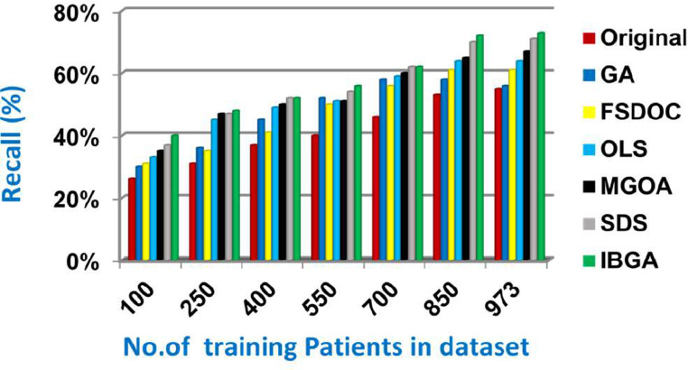
In this subsection, the IBGA that consists of Fscore method as a fast method and BGA as an accurate method will be evaluated and compared to many of the modern feature selection methods and also compared to the original dataset without feature selection (Original). The modern selection methods used in the comparison are Genetic Algorithm (GA) [2,27,28], Feature Selection via Directional Outliers Correcting (FSDOC) [36], Orthogonal Least Squares (OLS) based feature selection method [37], the Modified Grasshopper Optimization Algorithm (MGOA) [38], and Stochastic Diffusion Search (SDS) algorithm [29]. To evaluate these features selection methods, NB classifier is used as a standard method [29,30,31]. The Figs. (8→13) show the accuracy, error, precision, recall, and run-time of the used feature selection methods. IBGA outperforms other compared methods based on accuracy, precision, recall, and run-time performance metrics.
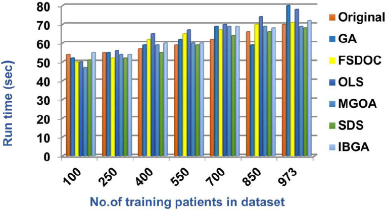
As shown in Figs. (8-12 ), at the maximum number of training data (e.g., 973 patients), accuracy values provided by Original, GA, FSDOC, OLS, MGOA, SDS, and IBGA are 0.59, 0.66, 0.69, 0.72, 0.80, 0.82, and 0.84 respectively. The best accuracy is introduced by IBGA while the worst accuracy is provided by Original. The main reason of these results is that IBGA selects the informative features before applying the NB classifier while Original contains all features in the dataset that includes irrelevant features. Accordingly, the error values of Original, GA, FSDOC, OLS, MGOA, SDS, and IBGA are 0.41, 0.34, 0.31, 0.28, 0.20, 0.18, and 0.16 respectively. Thus, IBGA can provide the maximum accuracy value and the minimum error value. At the maximum number of training data (e.g., 973 patients), the precision values of Original, GA, FSDOC, OLS, MGOA, and SDS are 0.54, 0.55, 0.60, 0.64, 0.67, and 0.70 respectively while IBGA provides 0.71. Accordingly, the best precision value is introduced by IBGA but the worst value is introduced by Original. According to the recall values, Original, GA, FSDOC, OLS, MGOA, SDS, and IBGA reach to 0.55, 0.56, 0.61, 0.64, 0.67, 0.71, and 0.73 respectively at the maximum number of training data (e.g., 973 patients). Thus, IBGA can provide the maximum recall value but Original can provide the minimum recall value. Fig. 13 shows that IBGA is faster than GA and OLS but it slower than Original, FSDOC, MGOA, and SDS, because GA and OLS need more iteration to get to the best subset of features. Thus, IBGA can provide the maximum accuracy, precision, and recall values but it cannot provide the minimum run time value even though it is faster than the basic GA method. At the end, Figs. (8-13) illustrate that IBGA can provide the best subset of features because it provides the highest accuracy value, and the lowest error value, but it cannot provide the lowest run time.
Fig. 12.
Recall of several feature selection methods.
Fig. 13.
Run time of several feature selection methods.
5.3. Testing the Covid-19 Prudential Expectation Strategy (CPES)
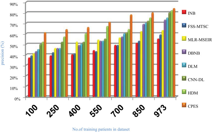
Evaluating CPES that composes of three phases, which are; (i) ORP, (ii) FSP, and (iii) CP will be performed in this section. To prove the effectiveness of CPES, several recently used Covid-19 classification strategies, which are Improved Naïve Bayes (INB) [31], Feature Subset Selection in Multivariate Time Series Classification (FSS-MTSC) strategy [39], Multivariate Logistic Regression on Modified SEIR (MLR-MSEIR) [40], DBNB [15], DLM [16], CNN-DL [17], and HDM [18] are compared to it. ORP uses HOR to reject outliers in the data and then FSP uses IBGA to select the best subset of features that only includes informative features without repetition. In fact, the number of selected features after implementing IBGA has been reduced to be 37 feature from the total number equals 50. At the end, the CP has been applied by using a new classification model called SNB to classify people based on their bodies’ reaction to Covid-19 infection. The Figs. (14→18) show the accuracy, error, precision, recall, and run-time of the used strategies. The effectiveness of CPES has been ensured in the results in which CPES is better than other compared strategies based on accuracy, precision, recall, and run-time performance metrics.
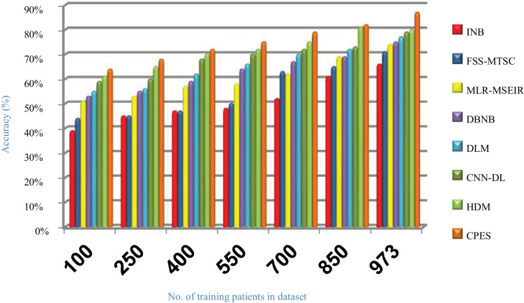
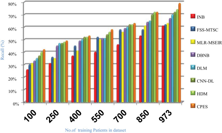
As shown in Figs. (14 –17 ), accuracy values provided by INB, FSS-MTSC, MLR-MSEIR, DBNB, DLM, CNN-DL, HDM, and CPES are 0.66, 0.71, 0.74, 0.75, 0.77, 0.79, 0.80 and 0.87 respectively at the maximum number of training data (e.g., 973 patients). According to these results, CPES achieves the best accuracy value depending on the use of two main phases, namely; outlier rejection phase and feature selection phase before applying the classification model to diagnose Covid-19 patients based on the individual vulnerability level to Covid-19. On the other hand, INB provides the worst accuracy value because it does not perform the feature selection process although it weights the features in the dataset. Also, INB does not perform the outlier rejection process on the dataset before learning the classification model. Accordingly, INB, FSS-MTSC, MLR-MSEIR, DBNB, DLM, CNN-DL, HDM, and CPES techniques introduce error values equal 0.34, 0. 29, 0.26, 0.25, 0.23, 0.21, 0.20 and 0.13 respectively. Hence, CPES can achieve the maximum accuracy value and the minimum error value. CPES introduces precision value reaches to 0.84 while INB, FSS-MTSC, MLR-MSEIR, DBNB, DLM, CNN-DL, and HDM give precision values reach to 0.55, 0.59, 0.63, 0.73, 0.75, 0.80, 0.82 respectively at the maximum number of training data (e.g., 973 patients). Thus, the best precision value is provided by CPES while the worst value is provided by INB because it does not use feature selection method or outlier rejection method. The recall values of INB, FSS-MTSC, MLR-MSEIR, DBNB, DLM, CNN-DL, and HDM are 0.61, 0.62, 0.63, 0.67, 0.70, 0.72, and 0.74 respectively but the recall value of CPES reaches to 0.79 at the maximum number of training data (e.g., 973 patients). Thus, INB provide the lowest recall value but CPES provides the highest recall value.
Fig. 15.
Error of several Covid-19 prudential expectation strategies.
Fig. 16.
Precision of several Covid-19 prudential expectation strategies.
Fig. 14.
Accuracy of several Covid-19 prudential expectation strategies.
Fig. 17.
Recall of several Covid-19 prudential expectation strategies.
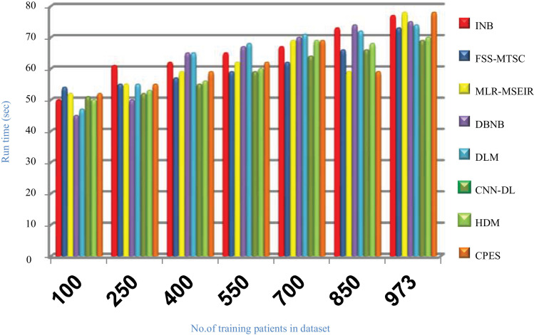
Fig. 18 illustrates that CPES is slower than other strategies which are INB, FSS-MTSC, MLR-MSEIR, DBNB, DLM, CNN-DL, and HDM. That is because the CPES depends on using outlier rejection method based on GWO method that consumes many iterations to reach to the best training data without outliers, also it depends on using feature selection method based on GA that needs many iterations to provide the best subset of features, and finally the statistical naïve Bayes is applied on the passed data after eliminating outliers and irrelevant features. In fact, spending time to implement ORP and FSP is not important to be taken into consideration for two reasons; (i) this time is only taken in the pre-processing stage before using the SNB classifier, and (ii) it helps the SNB to provide fast and accurate results depending on the filtered data. In other words, the ORP and FSP are executed in the CPES only once while SNB is continuously executed based on the passed data from ORP and FSP to classify patients. Finally, Figs. (14→18) illustrate that CPES is better than other recent strategies called INB, FSS-MTSC, MLR-MSEIR, DBNB, DLM, CNN-DL, and HDM. The reason is that CPES relies on filtering the dataset of irrelevant features and outliers using accurate methods before learning the diagnostic model which enables it to provide accurate results compared to other strategies. Hence, CPES provides the maximum accuracy, precision, recall values, and the lowest error value.
Fig. 18.
Run time of several Covid-19 prudential expectation strategies.
6. Conclusions and Future Work
The main objective of this paper is to introduce a new strategy called Covid-19 Prudential Expectation Strategy (CPES) for classifying individuals based on their bodies’ reaction to Covid-19 infection. CPES has three main phases, namely; Outlier Rejection Phase (ORP), Feature Selection Phase (FSP), and Classification Phase (CP). Outliers are eliminated from the input dataset through ORP using Binary Gray Wolf Optimization (BGWO). Then, an Improved Binary Genetic Algorithm (IBGA) has been used in the FSP to select the most significant features for improving the performance of the classification model and avoiding overfitting. Finally, the Statistical Naïve Bayes (SNB) classifier is employed in CP for individual classification based on the degree of their body response after infection with Covid-19. The experimental results have proven the effectiveness of the proposed CPES. Based on the obtained results, CPES outperforms the recent classification strategies based on accuracy, error, precision, and recall, which reach 0.87, 0.13, 0.84, and 0.79 respectively.
Perhaps the great advantage of the proposed CPES is its high efficiency of prediction, However, it has also several salient properties that other techniques do not have such as; (i) it is successfully qualifies it to be applied in hospitals and health centers due to its simplicity and straightforward implementation, (ii) CPES is scalable, hence it can be implemented to solve other prediction problems such as predicting the patient's health status after certain surgeries, (iii) The proposed strategy can be used in anticipating the spread of epidemics as well as protecting people at risk, hence, medical systems can take the necessary precautions (vi) besides its high diagnose accuracy, CPES has a high speed of diagnosis. On the other hand, this research introduces a new research field that can be successfully applied, especially in the medical field, which opens the door for others to research it. The new research field that was presented for the first time in this paper is to predict the health status of people if they were exposed to a particular disease before the actual infection. This new field of research is in line with the exponential acceleration in viruses evolution, and even the continuous discovery of new unknown viruses whose impact on people and their ability to spread cannot be expected.
Despite all these advantages, the proposed strategy suffers from a higher delay through the pre-processing stage compared with other techniques. The cause is that the pre-processing stage includes both ORP and FSP. However, employing ORP and FSP improves the model training. Moreover, this drawback has no essential effect because pre-processing is an offline stage, hence, it will not affect the diagnosing time. Also, the time factor is not the most important factor in diagnostic systems, where the most important factor is rather the accuracy of the diagnosis.
In the future, the proposed CPES strategy should be implemented on data collected from the Internet of Things (IoT) in a fog's cache server. This is intended to reduce the efforts of medical or healthcare systems because IoT can measure the body symptoms such as temperature, etc. in an automatic way to classify patients based on their bodies’ reaction to Covid-19 infection. Additionally, testing of the CPES strategy should be conducted using multiple datasets from different regions and at different sizes to ensure its overall usability. The methods used in ORP and FSP should be also further improved to be fast and to enable the CPES to be faster. We will communicate with medical institutions to adopt the presented strategy and actually implement it in order to take advantage of it to reduce the risk of Covid-19 disease.
Declaration of Competing Interest
The authors declare that they have no conflict of interest. ‘‘This paper does not contain any studies with human participants or animals performed by any of the authors.”
Acknowledgments
The authors are pleased to extend their big thanks to Mansoura University for the significant support. Special thanks of gratitude to President of Mansoura University for his unlimited support and his gentleness. Additionally, special thanks of gratitude to doctor Salah Abd Elghafar Mansour for his endless support and kindness. Also, we would like to express our special sincere thanks and gratitude to Dr. Omnia Anees Mansour for helping us throughout this work and giving us all the medical information that we need.
Biographies

Asmaa H. Rabie received a B. Sc. in Computers and Systems Engineering, with general grade Excellent with class honor in 2013. She got the master Degree in the area of load forecasting using data mining techniques in 2016 at Computers eng. and system dept, Mansoura University, Egypt. She got the Ph.D Degree in the area of load forecasting using data mining techniques in 2020 at Computers eng. and system dept, Mansoura University, Egypt. Her Interests (Programming Languages, Classification, Big Data, Data Mining, healthcare system, and Internet of Things), she is currently an lecturer in the faculty of Engineering, Mansoura University, Egypt.
E mail: asmaa91hamdy@yahoo.com
Faculty of Engineering, Mansoura University, Mansoura, Egypt

Nehal A. Mansour received a B. Sc. in Computer Engineering and Control Systems department from Mansoura University, Egypt with general grade Excellent with class honor. She got the master Degree in the area of data mining and artificial intelligence at Computer Engineering and Control Systems from Mansoura University, Egypt.
E-mail: nehal.anees.mansour@gmail.com

Ahmed I. Saleh received a B. Sc. in Computer Engineering and Control Systems from Mansoura University, Egypt with general grade Excellent. He got the master Degree and PhD Degree in the area of Mobile agent ad computing. His research interests include (Programming Languages, Networks and System Administration, and Database), he is currently a professor in the faculty of Engineering, Mansoura University.
E-mail: aisaleh@yahoo.com
Po. Box: 35516

Ali Takieldeen (IEEE Senior Member) received the PhD degree in Electronics and Communications Engineering in “Encryption and Data Security in Digital Communication Systems”. He has a lot of publications in various international journals and conferences. His current research interests are in multimedia processing, wireless communication systems, and Field Programmable Gate Array (FPGA) applications.
References
- 1.http://covid19.nilehi.edu.eg.
- 2.Mansour N., Saleh A., Badawy M., Ali H. Accurate detection of Covid-19 patients based on Feature Correlated Naïve Bayes (FCNB) classification strategy. Journal of Ambient Intelligence and Humanized Computing. 2021:1–33. doi: 10.1007/s12652-020-02883-2. https://link.springer.com/article/10.1007/s12652-020-02883-2 Springer. [DOI] [PMC free article] [PubMed] [Google Scholar]
- 3.Boccaletti S., Ditto W., Mindlin G., Atangana and. Modeling and forecasting of epidemic spreading: The case of Covid-19 and beyond. Chaos, Solitons & Fractals. 2020;135:1–2. doi: 10.1016/j.chaos.2020.109794. Elsevier. [DOI] [PMC free article] [PubMed] [Google Scholar]
- 4.Sun T., Wang Y. Modeling COVID-19 epidemic in Heilongjiang province, China. Chaos, Solitons & Fractals. 2020;138:1–5. doi: 10.1016/j.chaos.2020.109949. Elsevier. [DOI] [PMC free article] [PubMed] [Google Scholar]
- 5.Shaban W., Rabie A., Saleh A., Abo-Elsoud M. A new COVID-19 Patients Detection Strategy (CPDS) based on hybrid feature selection and enhanced KNN classifier. Knowledge-Based Systems. 2020;205:1–18. doi: 10.1016/j.knosys.2020.106270. Elsevier. [DOI] [PMC free article] [PubMed] [Google Scholar]
- 6.Hoehl S., Rabenau H., Berger A., Kortenbusch M., et al. Evidence of SARS-CoV-2 Infection in Returning Travelers from Wuhan, China. The new England journal of medicine. 2020;382(13):1278–1280. doi: 10.3390/healthcare9020196. [DOI] [PMC free article] [PubMed] [Google Scholar]
- 7.Huang C., Wang Y., Li X., Ren L., et al. Clinical features of patients infected with 2019 novel coronavirus in Wuhan, China. Lancet. 2020;395(10223):497–506. doi: 10.1016/S0140-6736(20)30183-5. [DOI] [PMC free article] [PubMed] [Google Scholar]
- 8.Castillo O., Melin P. Forecasting of COVID-19 time series for countries in the world based on a hybrid approach combining the fractal dimension and fuzzy logic. Chaos, Solitons & Fractals. 2020;(140):1–12. doi: 10.1016/j.chaos.2020.110242. Elsevier. [DOI] [PMC free article] [PubMed] [Google Scholar]
- 9.Shaban W., Rabie A., Saleh A., Abo-Elsoud M. Detecting COVID-19 patients based on fuzzy inference engine and Deep Neural Network. Applied Soft Computing. 2021;99:1–19. doi: 10.1016/j.asoc.2020.106906. Elsevier. [DOI] [PMC free article] [PubMed] [Google Scholar]
- 10.Rabie A., Ali S., Ali H., Saleh A. A fog based load forecasting strategy for smart grids using big electrical data. Cluster Computing. 2019;22(1):241–270. Springer. [Google Scholar]
- 11.Saleh A., Rabie A., Abo-Al-Ezb K. A data mining based load forecasting strategy for smart electrical grids. Advanced Engineering Informatics. 2016;30(3):422–448. Elsevier. [Google Scholar]
- 12.Castillo O., Melin P. A Novel Method for a COVID-19 Classification of Countries Based on an Intelligent Fuzzy Fractal Approach. healthcare. 2021;9(2):1–15. doi: 10.3390/healthcare9020196. [DOI] [PMC free article] [PubMed] [Google Scholar]
- 13.Wang Z., Xiao Y., Li Y., Zhang J., et al. Automatically discriminating and localizing COVID-19 from community-acquired pneumonia on chest X-rays. Pattern Recognition. 2021;110:1–9. doi: 10.1016/j.patcog.2020.107613. Elsevier. [DOI] [PMC free article] [PubMed] [Google Scholar]
- 14.Melin P., Castillo O. Spatial and Temporal Spread of the COVID-19 Pandemic Using Self Organizing Neural Networks and a Fuzzy Fractal Approach. Sustainability. 2021;13(15):1–17. [Google Scholar]
- 15.Shaban W., Rabie A., Saleh A., Abo-Elsoud M. Accurate Detection of COVID-19 Patients Based on Distance Biased Naıve Bayes (DBNB) Classification Strategy. Pattern Recognition. 2021;119:1–15. doi: 10.1016/j.patcog.2021.108110. Elsevier. [DOI] [PMC free article] [PubMed] [Google Scholar]
- 16.Alhwaiti Y., Siddiqi M., Alruwaili M., Alrashdi I., et al. Diagnosis of COVID-19 Using a Deep Learning Model in Various Radiology Domains. Complexity. 2021;2021:1–10. Wiley, Hindawi. [Google Scholar]
- 17.Shorfuzzaman M., Masud M., Alhumyani H., Anand D., et al. Artificial Neural Network-Based Deep Learning Model for COVID-19 Patient Detection Using X-Ray Chest Images. Journal of Healthcare Engineering. 2021;2021:1–16. doi: 10.1155/2021/5513679. Hindawi. [DOI] [PMC free article] [PubMed] [Google Scholar]
- 18.E.Carvalho R.Silva, Araújo F., Rabelo R., et al. An approach to the classification of COVID-19 based on CT scans using convolutional features and genetic algorithms. Computers in Biology and Medicine. 2021;136:1–11. doi: 10.1016/j.compbiomed.2021.104744. Elsevier. [DOI] [PMC free article] [PubMed] [Google Scholar]
- 19.Abualigah L., Yousri D., Abd Elaziz M., Ewees A. Aquila Optimizer: A novel meta-heuristic optimization algorithm. Computers & Industrial Engineering. 2021;157:1–37. Elsevier. [Google Scholar]
- 20.Abualigah L., Diabat A., Sumari P., Gandomi A. A Novel Evolutionary Arithmetic Optimization Algorithm for Multilevel Thresholding Segmentation of COVID-19 CT Images. Processes. 2021;9(7):1–37. [Google Scholar]
- 21.Park C. Outlier and anomaly pattern detection on data streams. The Journal of Supercomputing. 2019;75:6118–6128. Springer. [Google Scholar]
- 22.Shou Z., Li S. Large dataset summarization with automatic parameter optimization and parallel processing for local outlier detection. Concurrency Computation Practice and Experience. 2018;30(23):1–13. Wiley. [Google Scholar]
- 23.Abdel-Basset M., El-Shahat D., El-henawy I., de Albuquerque V., Mirjalili S. A new fusion of grey wolf optimizer algorithm with a two-phase mutation for feature selection. Expert Systems With Applications. 2020;139:1–14. Elsevier. [Google Scholar]
- 24.Mirjalili S., Mirjalili S., Lewis A. Grey Wolf Optimizer. Advances in Engineering Software. 2014;69:46–61. Elsevier. [Google Scholar]
- 25.El-kenawy E., Eid M., Saber M., Ibrahim A. MbGWO-SFS: Modified Binary Grey Wolf Optimizer Based on Stochastic Fractal Search for Feature Selection. IEEE Access. 2020;(8):107635–107649. IEEE. [Google Scholar]
- 26.Zhang Y., Meratnia N., Havinga P. Outlier Detection Techniques for Wireless Sensor Networks: A Survey. IEEE Communications Surveys & Tutorials. 2010;12(2):159–170. [Google Scholar]
- 27.Schulte R., Prinsen E., Hermens H., Buurke J. Genetic Algorithm for Feature Selection in Lower Limb Pattern Recognition. Frontiers in Robotics and AI. 2021;(8):1–12. doi: 10.3389/frobt.2021.710806. [DOI] [PMC free article] [PubMed] [Google Scholar]
- 28.Shreem S., Turabieh H., Al Azwari S, Baothman F. Enhanced binary genetic algorithm as a feature selection to predict student performance. Soft Computing. 2022:1–13. doi: 10.1007/s00500-021-06424-7. [DOI] [Google Scholar]
- 29.Shanthi S., Rajkumar N. Lung Cancer Prediction Using Stochastic Diffusion Search(SDS) Based Feature Selection and Machine Learning Methods. Neural Processing Letters. 2021;53:2617–2630. doi: 10.1007/s11063-020-10192-0. Springer. [DOI] [Google Scholar]
- 30.Blanquero R., Carrizosa E., Ramírez-Cobo P., Remedios M. Variable selection for Naïve Bayes classification. Computers & Operations Research. 2021;135:1–11. Elsevier. [Google Scholar]
- 31.Chen H., Hu S., Hua R., Zhao X. Improved naive Bayes classification algorithm for traffic risk management. EURASIP Journal on Advances in Signal Processing. 2021;30:1–12. Springer. [Google Scholar]
- 32.Sugahara S., Ueno M. Exact Learning Augmented Naive Bayes Classifier. entropy. 2021;23(1703):1–25. doi: 10.3390/e23121703. [DOI] [PMC free article] [PubMed] [Google Scholar]
- 33.Bhatia S., Malhotra J. Proceedings of the 2021 Third International Conference on Intelligent Communication Technologies and Virtual Mobile Networks (ICICV) IEEE; Tirunelveli, India: 2021. Naïve Bayes Classifier for Predicting the Novel Coronavirus; pp. 880–883. [Google Scholar]
- 34.Zhang H., Jiang L., Yu L. Attribute and instance weighted naive Bayes. Pattern Recognition. 2021;111:1–11. Elsevier. [Google Scholar]
- 35.Singh D., Singh B. Feature wise normalization: An effective way of normalizing data. Pattern Recognition. 2022;122:1–14. Elsevier. [Google Scholar]
- 36.Yuan L., Yang G., Q Xu, Lu T. Discriminative Feature Selection with Directional Outliers Correcting for Data Classification. Pattern Recognition. 2022:1–14. doi: 10.1016/j.patcog.2022.108541. Elsevier. [DOI] [Google Scholar]
- 37.Zhang S., Lang Z. Orthogonal least squares based fast feature selection for linear classification. Pattern Recognition. 2022;(123):1–18. Elsevier. [Google Scholar]
- 38.Sehgal S., Agarwal M., Gupta D., Sundaram S. Optimized grass hopper algorithm for diagnosis of Parkinson's disease. SN Applied Sciences. 2020;6(2):1–18. [Google Scholar]
- 39.Ircio J., Lojo A., Mori U., Lozano J. Mutual information based feature subset selection in multivariate time series classification. Pattern Recognition. 2020;108:1–12. Elsevier. [Google Scholar]
- 40.Palaniappan S., R V, David B., P S. Prediction of Epidemic Disease Dynamics on the Infection Risk Using Machine Learning Algorithms. SN Computer Science. 2022;47(3):1–3. doi: 10.1007/s42979-021-00902-3. Springer. [DOI] [PMC free article] [PubMed] [Google Scholar]


