Comparative poisson clinical trials of multiple experimental treatments vs a single control using the negative multinomial distribution

Abstract

This paper introduces a method which conditions on the number of events that occur in the control group to determine rejection regions and power for comparative Poisson trials with multiple experimental treatment arms that are each compared to one control arm. This leads to the negative multinomial as the statistical distribution used for testing. For one experimental treatment and one control with curtailed sampling, this is equivalent to Gail’s (1974) approach. We provide formulas to calculate exact one-sided overall Type I error and pointwise power for tests of treatment superiority and inferiority (vs the control). Tables of trial design parameters for combinations of one-sided overall Type I error = 0.05, 0.01 and pointwise power = 0.90, 0.80 are provided. Curtailment approaches are presented to stop follow-up of experimental treatment arms or to stop the study entirely once the final outcomes for each arm are known.

1 |. BACKGROUND

Clinical trials with several treatment groups frequently arise in drug and vaccine development, including late-phase (ie, Phase 3 and 4) studies. Using the Aggregate Analysis of ClinicalTrials.gov (AACT) database,¹ which collects protocol and results information for every clinical trial registered in ClinicalTrials.gov, we found that of the 213 647 interventional studies registered between September 17, 1999 and March 14, 2019 that reported the number of treatment arms in the trial, 42 737 (20.0%) had three or more arms. Of these, 28 112 also reported the phase of the trial, of which 8931 (31.8%) were categorized as Phase 3 or Phase 4.

When the primary outcome of a clinical trial is a rare binomial event or a Poisson outcome, the Poisson distribution may be used as the basis for statistical comparison of event rates in the treatment groups.^2–6 Such studies are referred to as comparative Poisson trials. Gail describes two approaches to conduct comparative Poisson studies with two treatments (eg, one experimental treatment compared to a control) under the assumption of equal subject allocation. Under “Design A”, the study continues until a prespecified total number of events have occurred among both groups; such studies will always result in a critical region of sufficient power provided that an appropriate total number of events is selected, but a definite termination date cannot be predetermined. Under “Design B”, the study continues until a prespecified termination time. Though the termination date is known exactly, this method can result in critical regions of insufficient power if few events have occurred among the groups at the time of stoppage,⁶ making Design B an unlikely choice for practical use. For both designs, the critical region and power computations are derived from the conditional binomial distribution.^2,6

To illustrate application of Gail’s Design A, consider a study comparing the efficacy of a new pertussis vaccine to a control vaccine in which the event rate is 0.01 (1 per 100 persons). The study is to have a one-sided Type I error of ≤0.05 to falsely find the new vaccine to be superior (ie, result in fewer cases of disease) to the control. Furthermore, assume the investigator wants to have 90% power to detect a risk ratio (ie, ratio of Poisson incidence rates) of the new vaccine to the control of 0.2. It is desirable to minimize follow-up to save time and money, which under Design A means to minimize the total number of pertussis cases that occur among both groups before the study is stopped and statistical comparison is made. If an equal number of subjects are allocated to each arm, then from Gail (1974) the study is stopped when 18 total pertussis events occur among both arms, with rejection of the null hypothesis of no difference in efficacy between the new pertussis vaccine and control if five or fewer events occur in the new vaccine arm. That is, subjects would be recruited over time and vaccinated with either the new intervention or the control in a 1:1 ratio and followed until 18 total events occur. If the new vaccine has similar efficacy as the control, this would require about 18 ÷ 0.01 = 1800 subjects to be recruited. If instead the alternative hypothesis is true and the new vaccine results in a lower rate of disease cases than the control, then more subjects would need to be recruited, as evidenced by the calculation 18 ÷ [(0.01 + 0.002)/2)] = 3000 subjects. If one were to use the curtailed sampling approach⁷ to conduct this study, then rather than wait for all 18 events to occur in both arms, the study would be stopped once either six events occur in the new pertussis vaccine arm (at which point rejection of the null hypothesis is impossible) or 18−5 = 13 events occur in the control arm (at which point the null hypothesis has been rejected). One of these stoppage points would occur at or sooner than 18 events occurring among both arms (and so reduces the number of subjects needed compared to an uncurtailed approach).

Now, suppose instead there were three versions of the new pertussis vaccine (eg, three different formulations of a pertussis vaccine or three different doses) to be compared to the control, and the objective is to design the study to have a one-sided overall Type I error of ≤0.05 to falsely find any of the new vaccines to be superior to the control. If none of the new vaccines are superior to the control, the tables in Gail will often produce greater than a 5% Type I error to falsely reject the null hypothesis for at least one of the new pertussis vaccines, since, as Dunnett noted for comparing multiple treatments to a control with continuous normally distributed outcomes, the Type I error for each new treatment vs the control will be partly additive.⁸ Thus, we develop an approach for controlling overall Type I error when comparing multiple treatments to one control in the comparative Poisson setting analogous to what Dunnett did for continuous outcomes.

Some methods for comparing multiple Poisson populations to a single reference group have been published,^9,10 but these methods are likely not operational for the clinical trials setting. Specifically, one method does not include power computations and appears limited to observational studies⁹ and the other uses a Bayesian framework which is limited by the choice of prior distribution and resulting asymptotic distribution used for statistical testing.¹⁰ Thus, the exact approach we propose in this paper for conducting comparative Poisson clinical trials of multiple experimental treatments vs a single control addresses a gap in the literature.

2 |. INTRODUCTION TO DESIGN C FOR TESTS OF MULTIPLE POISSON POPULATIONS

Accordingly, suppose there are K experimental treatment groups under study and the number of events D_k that occur in each is distributed Poisson(λ_k = i_kN_k), k = 1, 2, …, K, where i_k is the incidence rate of events per subject in the kth treatment group and N_k the number of subjects allocated to the kth treatment group. In the clinical trial setting, there is typically also a control group (either a placebo or standard of care treatment) which is used as a reference to determine the efficacy and/or safety of the experimental treatment(s). Thus, we also consider a control group for which there are allocated N_C subjects and the number of events is distributed Poisson(λ_C = i_CN_C). In such settings, directional alternative hypotheses are tested, where all contrasts are against the control group with rejection of the null hypothesis for each being one-sided in the same direction (eg, H₀ : i₁ = i₂ = … = i_K = i_C vs H_a : i_k < i_C for at least one k).

Hsu proposed in the appendix of her dissertation, but did not evaluate, a testing approach in which observation continues until the control group accumulates a prespecified number of events, denoted by d_C, at which time the trial is terminated.¹¹ This approach is denoted here as “Design C” to distinguish it from Gail’s Designs A and B (although with only one experimental treatment under curtailed sampling, the approach could be considered an expansion of Gail’s Design A where the study is stopped once a sufficient number of events occur in the control arm). In the case of two total treatment groups (ie, one experimental group vs one control group), testing under Design C is based on the negative binomial distribution. For multiple experimental treatment groups and a single control group and assuming equal subject allocation (ie, N₁ = N₂ = … = N_K = N_C), Hsu proves that the conditional distribution D₁, D₂, …, D_K | d_C is negative multinomial with parameters d_C,$\frac{i_C}{i_C+{\sum }_{k=1}^K{i}_k},\frac{i_1}{i_C+{\sum }_{k=1}^K{i}_k},\frac{i_2}{i_C+{\sum }_{k=1}^K{i}_k},\dots ,\frac{i_K}{i_C+{\sum }_{k=1}^K{i}_k}$. The derivation is based on three key facts¹²:

1. N_C | d_C ~ Gamma $\left(d_C,\frac{1}{i_C}\right)$ where N_C is the number of subjects required to obtain d_C events in the control group

2. D_k | N_C ~ Poisson(i_kN_C) for k = 1, 2, …, K and once the value of N_C is known, D_k no longer depends on d_C for k = 1, 2, …, K

3. Conditional on N_C = t, with t an observed value of the random variable N_C, the D_k are independent of one another

However, Hsu does not provide an approach for calculating the Type I error and power under this design. The objectives of this paper are, therefore, to formalize Design C by deriving formulas for Type I error and power for tests of treatment superiority and inferiority (vs the control) and to describe the practical implementation of the methodology.

3 |. TESTS OF TREATMENT SUPERIORITY UNDER DESIGN C

This section focuses on clinical trials where the primary objective is identifying any superior efficacy of one or more experimental treatments compared to a single control treatment in preventing a rare adverse binomial or Poisson outcome. As this is the first paper developing this design, we focus on the likely most common case of equal allocation of study participants to each of the K experimental treatment arms and control arm. The study will be stopped once a prespecified number d_C of events have occurred in the control group. At that time, an experimental treatment will be declared superior to the control if the number of events (eg, cases of disease) that have occurred in the experimental treatment group is significantly less than d_C. Based on these considerations, our global null and alternative hypotheses are

$$\begin{array}{l}{H}_0:i_1=i_2=\cdots =i_K=i_C\mathit{\text{vs}}\text{.}{H}_a:i_1=r_1{i}_C,i_2=r_2{i}_C,\dots ,i_K=r_K{i}_C\\ \text{where}\text{all}{r}_k\le 1\text{and}\text{at}\text{least}\text{one}\text{of}\text{the}{r}_k\text{is}\text{strictly}\text{less}\text{than}1\text{,}\end{array}$$ (1)

A more general version of Equation (1) for which the approach here applies would have all i_k ≥ i_C under H₀ and at least one i_k < i_C (or equivalently, at least one r_k < 1) under H_a. However, for simplicity in calculating Type I error (see Equation (5)), we will conservatively adhere to the strict equalities in H₀ in Equation 1.

The values r₁, …, r_K will be referred to as the “rate ratios” of the experimental treatment groups to the control group and represent the amount by which each of the K experimental treatments reduces the event incidence relative to the control treatment. Returning to the example of three new pertussis vaccines compared to one control, we have K = 3 and the hypotheses are H₀ : i₁ = i₂ = i₃ = i_C vs H_a : i₁ = r₁i_C, i₂ = r₂i_C, i₃ = r₃i_C where r₁, r₂, and r₃ are ≤1 and at least one of r₁, r₂, and r₃ are <1.

A global Type I error occurs when at least one experimental treatment is declared to be statistically superior to the control, when in fact it is not superior (ie, at least one of the three new pertussis vaccines is falsely declared superior to the control in our example). The global Type I error incurred for the hypotheses in Equation (1) (for the purposes of this paper, assuming no experimental treatment is superior to the control) will be termed “overall Type I error” and be denoted by α_ovr. A Type II error corresponds to failing to declare an experimental treatment superior to the control, when in fact that treatment is superior. We let ${\beta }_{T_k}$ denote making a Type II error on the kth individual experimental treatment for k = 1, 2, …, K. In our pertussis example with K = 3, ${\beta }_{T_1}$, ${\beta }_{T_2}$, and ${\beta }_{T_3}$ are the probabilities of failing to find the first, second, and third new vaccines, respectively, superior to the control when in fact the given treatment is superior. We define “pointwise power” to be the probability that an experimental treatment which has a given rate ratio r_k < 1 will be found to be superior to the control, that is, pointwise power for treatment $k=1-{\beta }_{T_k}$. In the pertussis example, if the study is designed to achieve a pointwise power of 0.9 with an assumed rate ratio of r_k = 0.2, then this means that the study will have at least 90% power to declare each new vaccine which has a true rate ratio ≤0.2 to be superior to the control. We design our test procedure to simultaneously control for a specified one-sided overall Type I error and achieve a desired level of pointwise power (see Section 5, Appendix 2, and Reference 12 for alternative power options).

The minimum number of events observed among the K experimental treatment groups (ie, minimum of the D_k, k = 1, 2, …, K) is a natural global test statistic for the hypotheses in Equation (1). That is, we will reject the null hypothesis of no difference in efficacy between any of the experimental treatments compared to the control treatment (in favor of the alternative hypothesis of at least one experimental treatment being superior to the control) if the minimum number of events that have occurred among the K experimental treatment groups by the time of study stoppage once the control group reaches d_C events is adequately small (say less than or equal to a value m). In fact, we will conclude that all experimental treatments with ≤ m events at the time of study stoppage are superior to the control. The one-sided overall Type I error is thus given by P(min(D₁, …, D_K) ≤ m) assuming the global null hypothesis is true for all K experimental treatments. It can be shown (see Appendix 1 of Data S1 for the derivations of all formulas in this paper) that this one-sided overall Type I error is given by:

$$1-{\int }_0^{\infty }\frac{t^{d_C-1}{e}^{-t}}{\Gamma \left(d_C\right)}{\left[1-\sum _{s=0}^m{e}^{-t}\frac{t^{\text{s}}}{s!}\right]}^{K}dt.$$ (2)

For a given value of d_C, we would find the largest value of m such that Equation (2) remains below the specified nominal α_ovr.

To compute the pointwise power for the test under a specified alternative for a given treatment arm k, that is, i_k = r_ki_C for some value of r_k < 1, we must determine the probability that the number of events D_k in that given experimental treatment group is sufficiently small (≤m) assuming that the incidence rate of events in the experimental treatment group is r_k-times as great as that in the control group. The corresponding formula for P(D_k ≤ m) under the alternative hypothesis is:

$${\int }_0^{\infty }\frac{t^{d_C-1}{e}^{-t}}{\Gamma \left(d_C\right)}\left[\sum _{s=0}^m{e}^{-r_{k}t}\frac{{\left(r_{k}t\right)}^s}{s!}\right]dt=\sum _{z=0}^m\left(\begin{array}{c}{d}_C+z-1\\ z\end{array}\right){\left(\frac{1}{1+r_k}\right)}^{d_C}{\left(1-\frac{1}{1+r_k}\right)}^z.$$ (3)

Due to the discrete nature of the test statistic, for the d_C that is chosen, the nominal overall Type I error (ie, the specified desired upper limit for α_ovr) will generally exceed the true overall Type I error achieved. For the same reason, the true pointwise power achieved will generally exceed the specified nominal pointwise power. For the pertussis example, if d_C = 16, m = 5, and r₁ = 0.2, then from Equations (2) and (3) (say being fit to achieve a one-sided overall Type I error of 0.05 and pointwise power of 0.8), the actual values are α_ovr ≈ 0.036 and ${\beta }_{T_1}\approx 0.123$ (ie, pointwise power ≈ 0.877). If we increase m to 6 with d_C = 16, then we have α_ovr ≈ 0.068 which exceeds 0.05 and ${\beta }_{T_1}\approx 0.061$ which has decreased. As such, our objective is to systematically find the smallest values of d_C (and thus also for m) for which both the actual α_ovr and ${\beta }_{T_k}$ simultaneously meet the desired nominal thresholds. Though other combinations of d_C and m will also satisfy the desired Type I error and pointwise power, choosing the smallest such d_C and associated m results in the smallest expected number of subjects to enroll, which implies economic and logistical gains.

Note that for small values of d_C, even taking m = 0 may exceed the nominal Type I error, and all values of m greater than zero will thus also exceed the nominal Type I error as Equation (2) is clearly increasing in m. However, as d_C is increased, eventually there are non-negative values of m that will satisfy the nominal Type I error and pointwise power. Accordingly, we wrote an R function, Des_Sup, for equal allocation Design C superiority trials (see Appendix 3 of Data S1 for the code) which takes the arguments K, nominal α_ovr, r, and nominal $1-{\beta }_{T_k}$ and sequentially increases the value of d_C and within each d_C, the value of m, until the smallest such combination that does not exceed the specified one-sided overall Type I error and is not less than the specified pointwise power is found. In addition to d_C and m, Des_Sup returns the true one-sided overall Type I error achieved and the true pointwise power achieved.

For the pertussis example with K = 3 new vaccines, a nominal one-sided overall Type I error of 0.05, a rate ratio of 0.2, and a nominal pointwise power of 0.9, the smallest d_C and corresponding m that satisfy the design specifications are 17 and 6, respectively. Hence, the superiority trial will be designed to allocate subjects to the control and each of the three new vaccine arms equally in a 1:1:1:1 ratio and proceed until d_C = 17 events are observed in the control group (at which time the study is stopped); the global null hypothesis will be rejected if the minimum number of events among the three new vaccine groups is less than or equal to the critical value of m = 6 at the time the control group reaches 17 events. Any new vaccine with no more than six events at the time of study stoppage would be declared superior to the control. The actual one-sided overall Type 1 error and pointwise power achieved are α_ovr ≈ 0.046 and $1-{\beta }_{Tk}\approx 0.925$, respectively.

But note that the number of events in each study arm might be monitored in real time and a new vaccine arm discontinued (ie, curtailed stoppage⁷) for futility to find superiority once it reaches m + 1 = 7 events before the control arm reaches 17 events; subsequent subjects would then be allocated equally to the remaining arms. Should all new vaccine arms reach 7 events before 17 events occur in the control, then the study can be stopped with none of the new vaccines being declared superior. Particularly in settings where few of the experimental treatment arms are effective, such futility discontinuation of arms can result in quicker and less expensive studies.

Note also that a common value of the rate ratio r was assumed for the three new vaccines (ie, r₁ = r₂ = r₃ = 0.2). We believe this is a reasonable assumption as, from a practical standpoint, the values of the r_k would be unknown in advance and thus would be determined by the level of efficacy the investigator determined needed to be detected (eg, that any new vaccine must reduce the incidence rate of events to a factor of r_k = 0.2 to be approved/marketable). While it could be argued that the values of the r_k might be chosen to vary if, for example, different treatments cost more or cause more adverse events, we believe it is likely that whenever this method is used the values of r_k input would be the same for all experimental treatments. As such, we defer further consideration of varying values of the r_k to Section 5.

The number of control group events d_C, critical value m, true one-sided overall Type I error achieved, and true pointwise power achieved in an equal allocation superiority trial conducted under Design C are presented in Table 1 for each combination of K = 1, 2, 3, 4, 5, nominal α_ovr = 0.05, 0.01, nominal pointwise power = 0.90, 0.80, and rate ratio r = 0.1, 0.2, 0.5. For the pertussis example presented above, the values of d_C, m, true one-sided overall Type I error, and true pointwise power are bolded in Table 1.

TABLE 1.

Number of control group events d_C and critical value m for the number of events in an experimental treatment arm to not exceed for rejecting H₀, true one-sided overall Type I error achieved, and true pointwise power achieved in an equal allocation superiority trial conducted under Design C for each combination of nominal α_ovr = 0.05, 0.01, nominal pointwise power = 0.90, 0.80, K = 1, 2, 3, 4, 5, and alternative hypothesis rate ratio r = 0.1, 0.2, 0.5

Nominal αovr = 0.05, Nominal Pointwise Power = 0.90
	r= 0.1		r= 0.2		r= 0.5
K	dC and m	True αovr and True 1 − βTk	dC and m	True αovr and True 1 − βTk	dC and m	True αovr and True 1 − βTk
1	dC =9	True αovr =0.0327	13	0.0481	47	0.0444
	m =2	True 1 − βTk =0.9288	5	0.9347	31	0.9054
2	10	0.0363	16	0.0485	56	0.0432
	2	0.9113	6	0.9395	36	0.9003
3	12	0.0471	17	0.0462	61	0.0460
	3	0.9588	6	0.9251	39	0.9034
4	13	0.0375	18	0.0394	63	0.0495
	3	0.9489	6	0.9088	40	0.9002
5	13	0.0453	18	0.0474	68	0.0454
	3	0.9489	6	0.9088	43	0.9035
Nominal αovr = 0.05, Nominal Pointwise Power = 0.80
	r= 0.1		r= 0.2		r= 0.5
K	dC and m	True αovr and True 1 − βTk	dC and m	True αovr and True 1 − βTk	dC and m	True αovr and True 1 − βTk
1	dC =7	True αovr =0.0352	10	0.0461	36	0.0435
	m =1	True 1 − βTk =0.8397	3	0.8419	22	0.8120
2	8	0.0369	13	0.0456	43	0.0488
	1	0.8058	4	0.8604	26	0.8151
3	11	0.0309	14	0.0415	47	0.0483
	2	0.8922	4	0.8318	28	0.8053
4	11	0.0397	15	0.0340	52	0.0463
	2	0.8922	4	0.8011	31	0.8147
5	11	0.0479	15	0.0410	54	0.0469
	2	0.8922	4	0.8011	32	0.8105
Nominal αovr = 0.01, Nominal Pointwise Power = 0.90
	r= 0.1		r= 0.2		r= 0.5
K	dC and m	True αovr and True 1 − βTk	dC and m	True αovr and True 1 − βTk	dC and m	True αovr and True 1 − βTk
1	dC =14	True αovr =0.0064	20	0.0096	70	0.0094
	m =3	True 1 − βTk =0.9378	7	0.9323	44	0.9006
2	15	0.0073	22	0.0079	82	0.0087
	3	0.9256	7	0.9031	51	0.9052
3	16	0.0064	24	0.0099	86	0.0090
	3	0.9122	8	0.9271	53	0.9004
4	16	0.0084	25	0.0085	91	0.0089
	3	0.9122	8	0.9140	56	0.9042
5	19	0.0061	27	0.0091	101	0.0084
	4	0.9478	9	0.9348	63	0.9270
Nominal αovr = 0.01, Nominal Pointwise Power = 0.80
	r= 0.1		r= 0.2		r= 0.5
K	dC and m	True αovr and True 1 − βTk	dC and m	True αovr and True 1 − βTk	dC and m	True αovr and True 1 − βTk
1	dC =12	True αovr =0.0065	15	0.0096	56	0.0096
	m =2	True 1 − βTk =0.8716	4	0.8011	33	0.8065
2	13	0.0072	19	0.0064	65	0.0097
	2	0.8498	5	0.8005	38	0.8089
3	14	0.0061	19	0.0094	69	0.0099
	2	0.8270	5	0.8005	40	0.8023
4	14	0.0079	22	0.0070	74	0.0097
	2	0.8270	6	0.8265	43	0.8119
5	14	0.0098	22	0.0086	78	0.0085
	2	0.8270	6	0.8265	45	0.8061

Abbreviations: d_C, number of stoppage events in the control arm; K, number of experimental treatment arms; w, critical value for each experimental treatment arm; reject H₀ for experimental arm k if D_k ≤ m and accept H₀ if D_k ≥ m + 1 at the time of study stoppage when the control arm reaches d_C events [D_k is the number of events that have occurred in experimental treatment group k at the time of study stoppage]; Nominal α_ovr and Nominal Pointwise Power are the threshold Type I error and pointwise power to achieve. True α_ovr is the actual Type I error and True 1 − β_Tk is the actual pointwise power attained due to discreteness of the distributions.

4 |. TESTS OF TREATMENT INFERIORITY UNDER DESIGN C

To derive a test of treatment inferiority (by which we mean identifying treatments that result in more rare adverse binary or Poisson outcomes than the control), again under equal allocation of study subjects across treatment groups, we must define the appropriate counterpart to the alternative hypothesis in Equation (1); that is, we must define the alternative hypothesis corresponding to at least one experimental treatment being inferior to the control. The hypotheses for an inferiority trial are, therefore, as follows:

$$\begin{array}{l}{H}_0:i_1=i_2=\cdots =i_K=i_{C}vs.H_a:i_1=r_1{i}_C,i_2=r_2{i}_C,\dots ,i_K=r_K{i}_C,\\ \text{where}\text{all}{r}_k\ge 1\text{and}\text{at}\text{least}\text{one}\text{of}\text{the}{r}_k\text{is}\text{strictly}\text{greater}\text{than}1\end{array}$$ (4)

A more general version of Equation (4) for which the approach here applies would have all i_k ≤ i_C under H₀ and at least one i_k > i_C (or equivalently, at least one r_k > 1) under H_a. However, for simplicity in calculating Type I error (see Equation (5) below), we will conservatively adhere to the strict equalities in H₀ in Equation (4).

These hypotheses may sometimes be relevant in Phase 1 or Phase 2 studies when evaluating several options to improve upon an existing standard of care treatment; researchers will want to know if a new treatment being considered in a study of several new treatments against one control is statistically proven inferior to the standard of care so that further resources are not invested in the new agent or other compounds which have a similar mechanism of action or chemical origin. These hypotheses may also be useful in safety studies where the rare outcome is an adverse event that occurs during treatment (eg, a study of adverse events of several dosage levels of a treatment compared to the standard dose of the regimen). For such studies, acceptance of the null hypothesis may indicate an acceptable safety profile of the experimental treatments.

It should be noted, however, that controlling the overall Type I error (as opposed to having the same numerical pointwise Type I error threshold for each experimental treatment) will make it more difficult to reject the null hypothesis and increases the Type II error, thus making it more difficult to identify truly inferior treatments. This is undesirable particularly for safety studies in which an increased number of experimental treatment arms makes it more difficult to declare a truly inferior individual experimental treatment to be more harmful than the control. Thus, in practice, researchers will need to ensure a high amount of power for such inferiority studies by recruiting an appropriate number of subjects based on sample size calculations to simultaneously manage the Type I and Type II errors.

If overall Type I error is managed, a natural global test statistic for the hypotheses in Equation (4) is the maximum of the D_k, k = 1, 2, …, K. That is, we will reject the null hypothesis and declare one or more of the experimental treatments to be inferior to the control if the maximum number of events among the K experimental treatment groups at the time the control group reaches d_C events is sufficiently large, say greater than or equal to a value w (in fact, we will conclude that all experimental treatments with ≥w events at the time of study stoppage once the control reaches d_C events are inferior to the control). To calculate the one-sided overall Type I error, we compute P(max(D₁, …, D_K) ≥ w) under the global null hypothesis in Equation (4) being true for all K experimental treatments, which yields:

$$1-{\int }_0^{\infty }\frac{t^{d_C-1}{e}^{-t}}{\Gamma \left(d_C\right)}{\left[\sum _{s=0}^{w-1}{e}^{-t}\frac{t^s}{s!}\right]}^{K}dt.$$ (5)

Pointwise power (the probability of finding the kth experimental treatment to be inferior to the control given that it has a rate ratio of r_k, that is, P(D_k ≥ w) under the specified alternative hypothesis) is given by:

$$1-{\int }_0^{\infty }\frac{t^{d_C-1}{e}^{-t}}{\Gamma \left(d_C\right)}\left[\sum _{s=0}^{w-1}{e}^{-r_{k}t}\frac{{\left(r_{k}t\right)}^s}{s!}\right]dt=1-\sum _{z=0}^{w-1}\left(\begin{array}{c}{d}_c+z-1\\ z\end{array}\right){\left(\frac{1}{1+r_k}\right)}^{d_C}{\left(1-\frac{1}{1+r_k}\right)}^z.$$ (6)

For a given d_C, an appropriate w can always be found that satisfies the nominal Type I error, as Equation (5) is clearly a decreasing function in w. However, this value may not satisfy a specified nominal pointwise power. But, as d_C is increased, eventually there is a value of w that will achieve the desired pointwise power. To conduct an inferiority test under Design C that controls for a specified one-sided overall Type I error and achieves a desired pointwise power, we find the smallest values of d_C and corresponding w that simultaneously satisfy Equations (5) and (6) for given nominal values of α_ovr and pointwise power. Again, for economic and logistical purposes it is better to have a smaller trial which translates to the smallest possible d_C and w.

The R function Des_Inf takes the same arguments as Des_Sup and returns d_C, the critical value w, the true one-sided overall Type I error achieved, and the true pointwise power achieved in an equal allocation inferiority trial conducted under Design C (see Appendix 3 of Data S1 for the code). For example, suppose there are K = 4 experimental treatments under study and researchers, subject to an overall Type I error threshold, want to determine if any of them have an unacceptable safety profile as indicated by causing significantly more adverse events than a control treatment. Suppose researchers aim to detect experimental treatments that cause at least twice as many adverse events as the control group (ie, r = 2) using a one-sided rejection region. To test the hypotheses in Equation (4) at a nominal one-sided overall Type I error of 0.05 and to achieve a minimum desired pointwise power of 0.9, the function Des_Inf(4, 0.05, 2,0.90) returns d_C = 41 and w = 63. Hence, the study would allocate subjects equally to the control and each of the experimental arms in a 1:1:1:1:1 ratio and continue until 41 events are observed in the control group. The global null hypothesis would be rejected (indicating at least one of the experimental treatments is significantly more harmful than the control) if 63 or more adverse events have occurred in any of the experimental treatment arms at the time the control arm reaches 41 events. The actual overall Type I error and pointwise power achieved are α_ovr ≈ 0.047 and 1 – β_Tk ≈ 0.9002, respectively.

Those treatments that have caused 63 or more adverse events by the time of study stoppage would be declared inferior to the control. Note also that adverse events in each treatment arm might likely be monitored in real time, with a given experimental treatment arm stopped if it reaches 63 events before the control arm reaches 41 events, and subsequent subjects then allocated equally to the remaining arms. If all experimental treatment arms reach 63 events before the control reaches 41, then the study is stopped with all experimental treatments being declared inferior.

Table 2 provides d_C, w, the true one-sided overall Type I error achieved, and the true pointwise power achieved in an equal allocation inferiority trial conducted under Design C for each combination of K = 1, 2, 3, 4, 5, nominal α_ovr = 0.05, 0.01, nominal pointwise power = 0.90, 0.80, and rate ratio r = 10, 5, 2. For the inferiority example above with K = 4 experimental treatments, the values of d_C, w, true one-sided overall Type I error, and true pointwise power are bolded in Table 2.

TABLE 2.

Number of control group events d_C and critical value w for the number of events in an experimental treatment arm to attain or exceed for rejecting H₀, true one-sided overall Type I error achieved, and true pointwise power achieved in an equal allocation inferiority trial conducted under Design C for each combination of nominal α_ovr = 0.05, 0.01, nominal pointwise power = 0.90, 0.80, K = 1, 2, 3, 4, 5, and alternative hypothesis rate ratio r = 10, 5, 2

Nominal αovr = 0.05, Nominal Pointwise Power = 0.90
	r= 10		r= 5		r= 2
K	dC and w	True αovr and True 1 − βTk	dC and w	True αovr and True 1 − βTk	dC and w	True αovr and True 1 − βTk
1	dC =3	True αovr =0.0327	6	0.0481	32	0.0444
	w =9	True 1 − βTk =0.9288	13	0.9347	47	0.9054
2	3	0.0342	7	0.0464	36	0.0498
	10	0.9113	16	0.9395	54	0.9039
3	3	0.0465	7	0.0428	40	0.0444
	10	0.9113	17	0.9251	61	0.9034
4	4	0.0332	7	0.0357	41	0.0472
	13	0.9489	18	0.9088	63	0.9002
5	4	0.0390	7	0.0421	44	0.0430
	13	0.9489	18	0.9088	68	0.9035
Nominal αovr = 0.05, Nominal Pointwise Power = 0.80
	r= 10		r= 5		r= 2
K	dC and w	True αovr and True 1 − βTk	dC and w	True αovr and True 1 − βTk	dC and w	True αovr and True 1 − βTk
1	dC =2	True αovr =0.0352	4	0.0461	23	0.0435
	w =7	True 1 − βTk =0.8397	10	0.8419	36	0.8120
2	2	0.0344	5	0.0434	27	0.0476
	8	0.8058	13	0.8604	43	0.8151
3	2	0.0466	5	0.0382	29	0.0463
	8	0.8058	14	0.8318	47	0.8053
4	3	0.0346	5	0.0472	30	0.0487
	11	0.8922	14	0.8318	49	0.8008
5	3	0.0406	5	0.0358	33	0.0440
	11	0.8922	15	0.8011	54	0.8105
Nominal αovr = 0.01, Nominal Pointwise Power = 0.90
	r= 10		r= 5		r= 2
K	dC and w	True αovr and True 1 − βTk	dC and w	True αovr and True 1 − βTk	dC and w	True αovr and True 1 − βTk
1	dC =4	True αovr =0.0064	8	0.0096	45	0.0094
	w =14	True − βTk =0.9378	20	0.9323	70	0.9006
2	4	0.0070	8	0.0076	52	0.0085
	15	0.9256	22	0.9031	82	0.9052
3	4	0.0099	9	0.0093	54	0.0088
	15	0.9256	24	0.9271	86	0.9004
4	4	0.0075	9	0.0078	57	0.0086
	16	0.9122	25	0.9140	91	0.9042
5	4	0.0090	9	0.0094	58	0.0089
	16	0.9122	25	0.9140	93	0.9020
Nominal αovr = 0.01, Nominal Pointwise Power = 0.80
	r= 10		r= 5		r= 2
K	dC and w	True αovr and True 1 − βTk	dC and w	True αovr and True 1 − βTk	dC and w	True αovr and True 1 − βTk
1	dC =3	True αovr =0.0065	5	0.0096	34	0.0096
	w =12	True 1 − βTk =0.8716	15	0.8011	56	0.8065
2	3	0.0068	6	0.0098	39	0.0095
	13	0.8498	18	0.8276	65	0.8089
3	3	0.0096	6	0.0088	41	0.0095
	13	0.8498	19	0.8005	69	0.8023
4	3	0.0071	7	0.0064	44	0.0093
	14	0.8270	22	0.8265	74	0.8119
5	3	0.0084	7	0.0077	45	0.0095
	14	0.8270	22	0.8265	76	0.8089

Abbreviations: d_C, number of stoppage events in the control arm; K, number of experimental treatment arms; w, critical value for each experimenstal treatment arm; reject H₀ for experimental arm k if D_k ≥ w and accept H₀ if D_k < w at the time of study stoppage when the control arm reaches d_C events [D_k is the number of events that have occurred in experimental treatment group k at the time of study stoppage]; Nominal α_ovr and Nominal Pointwise Power are the threshold Type I error and pointwise power to achieve. True α_ovr is the actual Type I error and True 1 − β_Tk is the actual pointwise power attained due to discreteness of the distributions.

As we believe establishing superiority of experimental treatments to a control will be the most likely usage of the Design C methodology in practice, we focus attention throughout the remainder of this paper to the superiority setting, occasionally making reference to the corresponding inferiority results.

5 |. CONSIDERATIONS FOR PRACTICAL IMPLEMENTATION OF DESIGN C

We now discuss a number of considerations for practical implementation of the Design C methodology. Firstly, recall that the methods presented above assumed equal allocation of subjects to the experimental and control arms. This assumption was made as (1) equal allocation is the most common allocation ratio used in practice¹³; (2) the simpler formulas that result from this assumption are sufficient for illustrating how to conduct comparative Poisson trials of multiple experimental treatments vs a single control under the Design C framework; (3) there is little justification for allocating more subjects to one experimental treatment and less to a different experimental treatment as this implies greater precision for some comparisons of each experimental treatment to the control¹¹ (though allocating an equal portion to the experimental treatment groups and a larger amount to the control may be a reasonable approach for reducing the expected amount of subjects required as has been noted in similar testing scenarios¹⁴); and (4) unequal subject allocation makes studies more difficult to blind. Although in practice an equal allocation ratio will likely not be exactly achieved, in most cases the deviations from equal allocation will be small enough so as to negligibly impact the Type I error and power calculated assuming an equal allocation ratio. However, all formulas presented in this paper are derived in Appendix 1 of Data S1 under a more general setting of unequal allocation of subjects to the treatment groups as this may be at least of theoretical interest.

Secondly, for the examples in Sections 3 and 4, we chose to power our tests using pointwise power, as we believe identifying treatment-wise those experimental treatments that achieve a specified rate ratio will be of most interest to researchers. However, other options for power exists, such as partial power (the probability that at least one truly superior/inferior experimental treatment is found to be superior/inferior, assuming that the relevant alternative hypothesis is true) and full power (the probability that all experimental treatments which are truly superior/inferior to the control are found to be superior/inferior, assuming that the relevant alternative hypothesis is true). Note that partial power coincides with definition (1) and full power coincides with definition (2) of the power for multiple testing situations suggested in Westfall and Young (p205), while pointwise power coincides with definition (4).¹⁵ Formulas for partial power and full power can be found in Appendix 2 of Data S1 and can be substituted for Equations (3) and (6) in the Design C testing procedure. It should be clear that for a fixed nominal value for α_ovr and a given nominal level of power, the design parameters d_C and m (or w) for a study designed with full power will generally be larger than in a corresponding study that uses pointwise power, and the design parameters for a study designed with partial power will generally be smaller than those required for a corresponding study using pointwise power.

Varying values of the alternative hypothesis rate ratios r₁, r₂, …, r_K can be accomodated in Design C studies under any of the aforementioned three types of power. If pointwise power is selected, then for superiority designs the study would typically be powered to detect any experimental treatments with a rate ratio ≤r, where r is chosen to be the same value for all experimental treatment arms; this common value would generally be selected as either the largest value of r_k that would be clinically acceptable or the largest expected value of r_k when different treatments have different anticipated levels of efficacy. If partial or full power are used, then (if needed) varying individual rate ratios r₁, r₂, …, r_K can be input directly into the power formula (see the formulas for partial and full power in Appendix 2 of Data S1).

Thirdly, it should be clear that Design C requires some level of unblinding (eg, a study monitor may be unblinded to the identity of the control group so as to stop the trial once d_C events are accrued in the control group). However, we believe that this is likely not problematic in most cases as (1) Phase 1 studies are usually conducted in an open-label fashion, and even Phase 2 and 3 studies may be conducted as open-label,¹⁶ and (2) clinical trials may have a designated unblinded statistician/study manager to monitor study progress independently of blinded personnel or may utilize an independent, unblinded data monitoring committee to ensure the integrity of trial data and to evaluate safety signals that may be treatment-dependent.¹⁷

In addition, we now propose the following approach to study conduct that achieves partial blinding: if a subject experiences the event of interest, then unblind only that subject. If m + 1 subjects are unblinded in an experimental treatment group, then all subjects allocated to that treatment group can be unblinded and enrollment into and follow-up of that experimental treatment arm can be terminated; H₀ is accepted for that experimental treatment. The trial continues until either (1) d_C subjects in the control group are unblinded, at which time all experimental treatments which are still active (ie, that have not been discontinued due to having m + 1 subjects experience the event of interest) are declared superior to the control, or (2) all experimental treatment groups have been discontinued due to having m + 1 subjects experience the event of interest, and so it will no longer be possible to reject the null hypothesis for any experimental treatment group even if one were to wait for d_C subjects in the control group to experience the event of interest. This procedure ensures that no study personnel need to be unblinded to the treatment allocation schedule at the start of the study and limits the amount of unblinding during the study.

Lastly, as mentioned in Section 2, conditional on N_C (the number of subjects needed for the control group to reach d_C events) the D_k are independent of one another and so a decision to reject or accept the null hypothesis for each individual experimental treatment group vs the control is separately obtained via integration over the density of N_C | d_C under Design C. That is, when the study is stopped once the control group reaches d_C events (or possibly sooner if curtailment is applied) any experimental treatment groups with ≤ m (respectively, ≥ w) events will be declared superior (respectively, inferior) to the control independently of the number of events in a different experimental treatment arm. This contrasts a primary limitation of extending Gail’s Design A to multiple treatments vs a single control where stoppage is based on the total number of events in all arms combined.

If Design A were applied to such settings (ie, waiting for a specified total number of events to occur among the experimental and control groups combined before terminating the study) there may be situations in which a particular experimental treatment group k is responsible for the majority of events. For example, consider a superiority study under Design A in which there are four experimental treatments to be compared to a single control and the total number of events to be observed to stop the study is 30. If the first experimental treatment group is responsible for 26 of the 30 total events, then it is clear that the first experimental treatment group is not superior (and in fact is greatly inferior) to the control. But with only four remaining events distributed among the control and other treatment arms, there is little (in fact, no) ability to draw conclusions about the superiority of the remaining three experimental treatment groups relative to the control. In comparison, Design C by conditioning on the number of events in the control group guarantees a large enough number of events can occur in the control (and experimental treatments arms) so that the ability to determine treatment superiority/inferiority for treatment group i is not adversely impacted by the number of events observed in treatment group j for all j ≠ i.

6 |. DISCUSSION

We now present some exploratory analyses of the relationships between the design parameters for tests of treatment superiority under Design C and indicate some additional ways that the methodology can be applied to clinical trials.

We generated the superiority trial design parameters for combinations of α_ovr = 0.05, 0.025, 0.01, pointwise power = 0.90, 0.80, and K = 1, 2, …, 10 and found that when the value of K is held constant and the rate ratio r is varied from 0.05 to 0.5 (in increments of 0.05), the values of d_C and m both increased in an approximately quadratic manner. This is evidenced in Figure 1 which displays the values of d_C and m for the case α_ovr = 0.05, pointwise power = 0.9, and K = 1, 5, 10 (graphs created for other parameter combinations featured similar trends and are omitted). These increases in d_C and m imply that for a fixed number of treatment groups, as the value of the rate ratio arithmetically increases, the expected number of subjects to be enrolled increases at an accelerated rate and so does the time needed for the study to terminate (as it takes longer for the control group to reach d_C events or, in the case of a curtailed trial, it takes longer for the experimental treatment groups to reach the futility boundary of m + 1 events).

FIGURE 1.

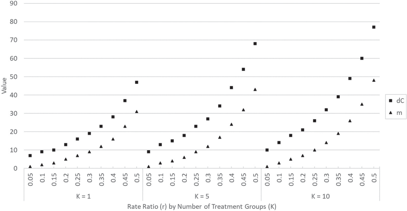
Values of d_C and m for a Design C superiority trial with parameters α_ovr = 0.05, pointwise power = 0.9, r = 0.05, 0.1,…, 0.5, and for fixed values of K (K = 1, 5, 10)

We evaluated combinations of α_ovr = 0.05, 0.025, 0.01, pointwise power = 0.9, 0.80, and r = 0.1, 0.2, 0.3, 0.4, 0.5 and found that when the value of r was held constant and K ranged from 1 to 20, the values of d_C and m increased relatively slowly (with greater rates of increase observed at higher values of r). This can be seen in Figure 2 which displays the values of d_C and m for α_ovr = 0.05, pointwise power = 0.9, r = 0.1, 0.3, 0.5 and for values of K ranging from 1 to 20. While these linear increases imply longer studies, this is occurring at a less accelerated rate than when the value of r being tested for under the alternative hypotheses is increased. In addition, as the underlying distribution is discrete with the true Type I and Type II errors often being conservative, small increases in the value of the alternative rate ratio do not necessarily result in an increase in d_C and m as the same values can generate less conservative errors that still meet the required thresholds.

FIGURE 2.

Values of d_C and m for a Design C superiority trial with parameters α_ovr = 0.05, pointwise power = 0.9, K = 1, 2,…, 20, and for fixed values of r (r = 0.1, 0.3, 0.5)

Overall, the rate of increase with K was somewhat larger for d_C compared to m (as evidenced by the slopes of the lines of best fit in Figure 2 for the case of r = 0.5). This implies that for curtailed studies, as the value of K increases the ability to stop follow-up of ineffective treatments early is slowly diminished since the value of m increases slowly. In contrast, for effective treatments, it takes longer to prove their superiority when d_C increases as it takes relatively longer for the control group to reach d_C (the point at which effective treatments can be declared superior to the control).

We now note some relationships between the design parameters for Design C superiority and inferiority trials. Here we let $d_C^S$ and $d_C^I$ denote the number of control group events to observe in a superiority study and inferiority study, respectively, and r^S and r^I denote the rate ratios under the superiority and inferiority settings, respectively. For studies with K = 1 and for any combination of nominal α_ovr and nominal pointwise power, $d_C^S$ and m can be obtained via $d_C^S=w$ and $m=d_C^I-1$ when r^S = 1/r_I, and the same true α_ovr and pointwise power are obtained under the corresponding superiority and inferiority designs (see Tables 1 and 2). This is due to the fact that the superiority and inferiority hypotheses are equivalent parameterizations. For example, testing that (1) Treatment A is twice as effective as Treatment B is equivalent to testing that (2) Treatment B is half as effective as Treatment A. The fact that $m=d_C^I-1$ rather than $m=d_C^I$ is due to nonsymmetry in the way we defined our rejection regions (ie, using rejection for ≤ m or ≥ w for superiority and inferiority, respectively, rather than requiring strict inequality for one of the directions).

However, for K = 2, 3, 4, 5 with the same nominal α_ovr and nominal pointwise power under the superiority and inferiority settings and r^S = 1/r^I, the relationships noted for K = 1 do not always hold due to the nonsymmetry of the gamma distributions being integrated in each direction (ie, superiority and inferiority directions) and exponentiating the different densities to a K > 1 power creates an inequality over the reversed rejection region (even though for K = 1 they integrate to the same value). However, for the same nominal α_ovr and nominal pointwise power and r^S = 1/r^I, when the value of $d_C^S$ in Table 1 does happen to coincide with the value of w in Table 2 (and in such cases, m is found to equal $d_C^I-1$), the true pointwise power is the same. This is because the pointwise power is a one-to-one comparison (ie, represents the probability of finding a given individual experimental treatment group to be superior/inferior to the control). In these cases, with the same rejection regions and parameters reversed, the probability to find one experimental treatment with rate ratio r^S superior to the control is the same as the probability to find an experimental treatment with rate ratio 1/r^S inferior to the control.

As previously mentioned, Design C studies can be implemented with curtailed stoppage of treatment arms, that is, enrollment in and follow-up up of individual treatment arms can be terminated once the ultimate decision regarding rejection or acceptance of the null hypothesis is known for a given treatment arm (and the entire trial can be stopped once the ultimate decision is known for all treatment arms).⁷ For Design C superiority studies, this means that recruitment into and follow-up of each experimental treatment arm can be discontinued once the number of events exceeds the critical value (ie, once the number of events reaches m + 1) as it will no longer be possible to reject the null hypothesis for this experimental treatment group, and the entire trial can be terminated once either (i) all experimental treatment arms reach m + 1 events as it will then no longer be possible to reject the global null hypothesis, even if the study were to continue until all d_C events are observed in the control group, or (ii) the control group reaches d_C events at which time the trial is stopped and all remaining active experimental treatment arms (ie, that have not reached m + 1 events) are declared superior to the control.

For a curtailed superiority trial, the expected number of subjects needed to generate the required events to complete the study under the alternative hypothesis is always greater than the expected number under the null hypothesis. Under the null hypothesis, all experimental treatment groups tend to accumulate events at the same rate as the control group, whereas under the alternative hypothesis, events in the experimental treatment groups tend to accumulate at rates lower than that of the control group. Hence, it takes longer under the alternative hypothesis for the experimental treatment arms to reach m + 1 events, the time at which follow-up of these treatment arms can be terminated, than under the null hypothesis. The gain in conducting a curtailed study vs an uncurtailed study is also greatest when there are one or more ineffective experimental treatments for similar reasons. A more thorough discussion of the properties of a curtailed study under Design C and estimation of the expected number of subjects required would be the topic of a new paper (see Reference 12 for additional comments on curtailment in Design C studies, including consideration of curtailment in inferiority studies).

We next note that the Bonferroni approach can be implemented under Design C. The Bonferroni procedure conducts each individual test (ie, comparison of each experimental treatment to the control) at significance level α_individual = α_ovr/K to conservatively control the familywise error rate¹⁸ and can be used as an approximation to our exact Design C method. It could be argued that the Bonferroni procedure is simpler to implement than the exact approach as comparing an individual experimental treatment to the control is accomplished via the univariate negative binomial distribution.

For the previous pertussis example, we can determine the design parameters for the trial under the Bonferroni approach by setting the number of experimental treatment groups equal to one and the nominal Type I error equal to $\frac{{\alpha }_{\text{ovr}}}{K}=\frac{0.05}{3}$ in Des_Sup. The resulting parameters are d_C = 18 and m = 6. Notice that the number of control events to be observed is larger than under the exact approach (d_C = 17). In other scenarios, it is also possible to find a larger critical value m under the Bonferroni procedure compared to the exact approach. A larger d_C or m indicates that it will take more expected subjects to power the trial and thus increased study costs. However, due to the discrete nature of the testing approach, the values of d_C and m may coincide under the Bonferroni and exact approaches (see Reference 12 for examples); thus, applying Design C under the Bonferroni approach may be a viable practical option in some specific scenarios. Alternatively, a less-conservative approach such as a sequential testing procedure¹⁹ or the Benjamini-Hochberg procedure²⁰ for multiple comparisons might yield results closer to the exact approach described in this paper, but this would be a topic for future research.

The Bonferroni approach can also be applied to control the overall Type I error of two-sided tests comparing multiple experimental treatments to one control. For example, repeated one-sided overall Type I error of 0.025 could be used to obtain a two-sided Type I error of 0.05 by combining the one-sided superiority and inferiority tests described in Sections 3 and 4. In such cases, treatments can be tested for superiority relative to the control if a sufficiently small number of events are observed in an experimental treatment arm, but can also be declared inferior if too many events are observed in an experimental treatment arm. By the Bonferroni approach, the overall Type I error is controlled.

7 |. CONCLUSION

This paper presents an operational method for conducting comparative Poisson clinical trials of multiple experimental treatments vs a single control treatment based on conditioning on the number of events observed in the control group, leading to inference via the negative multinomial distribution. This method will always yield a critical region of sufficient power (given appropriate choices of d_C and m [or w]). In addition, due to the independence of the treatment groups achieved by conditioning on N_C, a declaration of superiority/inferiority relative to the control can be made for each individual experimental treatment while maintaining a one-sided overall Type I error. Lastly, the ability to implement Design C under curtailed stopping rules (ie, terminating study arms that exceed m + 1 events in a superiority study or reach w events in an inferiority study in real time) implies reduced expenses and/or quicker trials.

DATA AVAILABILITY STATEMENT

The data that support the findings of this study are available in the Aggregate Analysis of ClinicalTrials.gov (AACT) public database at https://aact.ctti-clinicaltrials.org/download. These data were derived using the March 16, 2019 daily pipe-delimited file (monthly archives for the data are available at https://aact.ctti-clinicaltrials.org/pipe_files). Additionally, the authors affirm that the Des_Sup and Des_Inf codes that support the findings of this study are available in Supporting information to this article (see Appendix 3 of Data S1 for the code).²¹

REFERENCES

- 1.Access to Aggregate Content of ClinicalTrials.gov (AACT) Clinical trials transformation initiative. https://www.ctti-clinicaltrials.org/aact-database. Accessed March 16, 2019.
- 2.Przyborowski J, Wilenski H. Homogeneity of results in testing samples from Poisson series. Biometrika. 1940;31(3–4):313–323. [Google Scholar]
- 3.Birnbaum A Some procedures for comparing Poisson processes or populations. Biometrika. 1953;40(3–4):447–449. [Google Scholar]
- 4.Birnbaum A Statistical methods for Poisson processes and exponential populations. J Am Stat Assoc. 1954;49(266):254–266. [Google Scholar]
- 5.Lehmann EL, Scheffé H. Unbiasedness: theory and first applications. Testing Statistical Hypotheses. 3rd ed. New York, NY: Springer; 2005:110–149. [Google Scholar]
- 6.Gail M Power computations for designing comparative Poisson trials. Biometrics. 1974;30(2):231–237. [Google Scholar]
- 7.Herrmann N, Szatrowski TH. Curtailed binomial sampling procedures for clinical trials with paired data. Control Clin Trials. 1985;6(1):25–37. [DOI] [PubMed] [Google Scholar]
- 8.Dunnett CW. A multiple comparison procedure for comparing several treatment with a control. J Am Stat Assoc. 1955;50(272):1096–1121. [Google Scholar]
- 9.Suissa S, Salmi R. Unidirectional multiple comparisons of Poisson rates. Stat Med. 1989;8:757–764. [DOI] [PubMed] [Google Scholar]
- 10.Singh B Bayesian inference for comparing several treatment means under a Poisson model. Commun Stat-Theor M. 1980;9:1137–1145. [Google Scholar]
- 11.Hsu T Comparative Poisson Trials for Comparing Multiple New Treatments to the Control [dissertation]. New Brunswick: Rutgers University; 2010. [Google Scholar]
- 12.Chiarappa J Application of the Negative Multinomial Distribution to Comparative Poisson Clinical Trials of Multiple Experimental Treatments Versus a Single Control [dissertation]. New Brunswick: Rutgers University; 2019. [Google Scholar]
- 13.Altman G Avoiding bias in trials in which allocation ratio is varied. J R Soc Med. 2018;111(4):143–144. [DOI] [PMC free article] [PubMed] [Google Scholar]
- 14.Hoover DR, Blackwelder WC. Allocation of subjects to test null relative risks smaller than one. Stat Med. 2001;20:3071–3082. [DOI] [PubMed] [Google Scholar]
- 15.Westfall PH, Young SS. Further topics. Resampling-Based Multiple Testing: Examples and Methods for p-Value Adjustment. New York, NY: Wiley; 1993:184–216. [Google Scholar]
- 16.Umscheid CA, Margolis DJ, Grossman CE. Key concepts of clinical trials: a narrative review. Postgrad Med J. 2011;123(5):194–204. [DOI] [PMC free article] [PubMed] [Google Scholar]
- 17.Lin JY, Lu Y . Establishing a data monitoring committee for clinical trials. Shanghai Arch Psychiatry. 2014;26(1):54–56. [DOI] [PMC free article] [PubMed] [Google Scholar]
- 18.Lehmann EL, Scheffé H. Multiple testing and simultaneous inference. Testing Statistical Hypotheses. 3rd ed. New York, NY: Springer; 2005:348–391. [Google Scholar]
- 19.Wald A Sequential tests of statistical hypotheses. Breakthroughs in Statistics. Foundations and Basic Theory. Vol 1. New York, NY: Springer; 1992:256–298. [Google Scholar]
- 20.Benjamini Y, Hochberg Y. Controlling the false discovery rate: a practical and powerful approach to multiple testing. J R Stat Soc. 1995;57(1):289–300. [Google Scholar]
- 21.Hoover DR. Subject allocation and study curtailment for fixed event comparative Poisson trials. Stat Med. 2004;23(8):1229–1245. [DOI] [PubMed] [Google Scholar]
Associated Data
This section collects any data citations, data availability statements, or supplementary materials included in this article.
Supplementary Materials