Abstract
Most people with low vision rely on their remaining functional vision for mobility. Our goal is to provide tools to help design architectural spaces in which safe and effective mobility is possible by those with low vision---spaces that we refer to as visually accessible. We describe an approach that starts with a 3D CAD model of a planned space and produces labeled images indicating whether or not structures that are potential mobility hazards are visible at a particular level of low vision. There are two main parts to the analysis. The first, previously described, represents low-vision status by filtering a calibrated luminance image generated from the CAD model and associated lighting and materials information to produce a new image with unseen detail removed. The second part, described in this paper, uses both these filtered images and information about the geometry of the space obtained from the CAD model and related lighting and surface material specifications to produce a quantitative estimate of the likelihood of particular hazards being visible. We provide examples of the workflow required, a discussion of the novelty and implications of the approach, and a short discussion of needed future work.
Keywords: low vision, visual acuity, mobility, architecture, lighting, accessibility, universal design
1. Introduction
Low Vision refers to any long-term visual impairment, not correctable by glasses or contacts, which affects every day functioning. In more quantitative terms, low vision is often defined as visual acuity less than 20/40 (metric 6/12) or a visual field with a maximum extent of less than 20° in the better eye. Low vision refers to people with remaining functional vision and does not include people who are totally blind. Prevalence statistics on visual impairment usually combine low vision and total blindness. Of the 441.5 million visually-impaired people worldwide, the vast majority have low vision [Bourne 2017]. By recent estimates, there are about 5.7 million Americans with impaired vision, most of whom have low vision [Chan 2018]. Because the prevalence is high for older people, this number is expected to nearly double by 2050 [Chan 2018].
There is a broad and growing interest in architectural and environmental design that facilitates safe and effective mobility by people with low vision [NIBS 2015]. By analogy to principles for enhancing physical accessibility, our research focuses on designing visually accessible spaces. We define the visual accessibility of an environment as the degree to which vision supports travel efficiently and safely through the environment, assists in the perception of the spatial layout of key features in the environment, and helps to keep track of one’s position and heading in the environment. The major factors affecting visual accessibility include the vision status of the pedestrian (including acuity, contrast sensitivity and field of view), geometrical properties of the architectural design (including landmarks, objects and obstacles), the nature and variation of lighting (natural and artificial), surface properties (including color, texture, gloss), and contextual cues (such as the visible presence of a railing signifying the presence of steps even if the steps themselves are not visible). Our goal is to provide tools to enable the design of safe environments for the mobility of low-vision individuals and to enhance safety for others, including older people with normal vision, who may need to operate in visually challenging conditions.
In this paper, we describe the development of a computer-based design tool for identifying potential mobility hazards in public spaces such as a hotel lobby, subway station, or eye-clinic reception area that may be difficult or impossible to see by low vision individuals. This analysis can be performed at the design phase of a project, where corrections are often far easier than after construction has been completed. Ultimately, we hope that such tools can assist the architectural design professions in evaluating and improving visual accessibility, thereby enhancing mobility and quality of life for people with low vision.
Low vision can result from a wide range of eye and vision disorders. The functional consequences of low vision include reductions in acuity, contrast sensitivity, and visual-field loss. Acuity is the most widely used metric for visual impairment, and often the only measure readily available concerning an individual person with low vision or available as a standard of visibility. Recent quantitative models of pattern visibility in both normal and low vision rely on measures of contrast sensitivity across a range of spatial frequencies, as summarized in the human contrast sensitivity function (Campbell and Robson, 1968). In the computational flow described in this paper, visual deficits are represented by embedding contrast-sensitivity functions for low-vision observers in the computational flow. By so doing, we are focusing on identifying features seen or not seen by people with specified levels of acuity and contrast sensitivity.
Acuity refers to the ability to see fine detail. In clinical settings, it is commonly quantified using a Snellen fraction (e.g., normal visual acuity is 20/20 in the U.S. or 6/6 in metric units). Increases in the denominator of the Snellen fraction correspond to decreases in acuity. 20/40 can be taken as the boundary for low vision. LogMAR values, which are a logarithmic scale for acuity are also used, with normal vision indicated by logMAR 0.0 and numerically increasing logMAR numbers corresponding to decreases in acuity. For instance, the logMAR value corresponding to 20/40 acuity is log10(2) = 0.30. Contrast sensitivity refers to the ability to see small changes in luminance. One common way to quantify contrast sensitivity is the score obtained from the Pelli-Robson chart [Pelli, Robson, & Wilkins, 1988], which is a logarithmic scale in which 0.0 corresponds to an ability to see only the highest possible contrast and 2.0 corresponds to normal vision.
Our approach to evaluating hazard visibility for low vision, described below, makes use of measures of acuity and contrast sensitivity. In the Discussion section, we will consider two limitations of this approach. First, we do not take patterns of visual-field loss into account. Someone with a severely restricted field of view may miss seeing a hazard, such as a step, because some or all of the hazards are not in their field of view. Second, in real-world scenarios, lighting variations, visual light and dark adaptation, glare, and other variables may compromise to some extent clinical estimates of acuity and contrast sensitivity.
When considering visibility, architects and lighting designers typically use illuminance-based design practices that focus on the intensity of illumination sources and the reflectivity of surface materials. Illuminance-based design evaluates the total luminous flux incident to a surface and does not take into account the interaction of light with the surface’s material properties. In particular, illuminance-based design does not consider the interaction between illuminance, surface reflectance, surface geometry, and viewpoint. Luminance-based design, on the other hand, evaluates the intensity of light emitted from a surface in a given direction and better represents what we see. The visibility of hazards and other features depends on the angular size of these features at the viewpoint in question and the luminance contrast between the feature and its surround. With low vision, inadequate angular size and contrast differences often make hazards impossible to see. Thus, luminance-based design approaches in which the careful positioning of light sources, surfaces, and the viewer, together with the specific optical properties of the surfaces, can have a profound effect on low-vision visibility.
Figure 1, produced using the Radiance Rendering System [Ward & Shakespeare, 1998], illustrates the importance of luminance-based design. On the left is a box with the materials on each side having the indicated reflectivity. In the center image, rendered with a 2’ x 4’ lensed down light, the structure of the box is clearly visible. In the right image, the light source has been moved 2’ horizontally closer to the box. Now, there is no visible boundary between the top and right surfaces at the surface joint marked by the arrow, despite the large difference in reflectivity. A design process that fails to note the poor visibility of two adjacent surfaces differing by a factor of four in reflectivity is going to be hard pressed to expose potential problems with hazard visibility, particularly for low vision viewers.
Figure 1.
Illumination and reflectivity alone are not enough to predict visibility. Two surfaces under the same illumination but differing in reflectance by a factor of 4X can look the same.
As pointed out in a report by the National Institute of Building Sciences [NIBS 2015], “luminance-based design is not well understood by designers, partly because there are few computer programs that model luminance in a way that is practical for use as a design tool.” Low vision involving loss of acuity adds additional problems for the designer. For example, a feature representing a potential trip hazard may present a challenge for someone with low vision if it subtends too small a visual angle from viewpoints on the approach path, even if it is well lit and has a luminance contrast distinct from its immediate surround. In this paper, we describe a system that addresses these limitations. Our novel approach, unavailable in current design systems, integrates the quantitative photometry of luminance-based design with empirical investigations of low vision to predict the visibility of mobility hazards during the design process.
The difficulty of quantifying the relationship between visibility and lighting has long been recognized (e.g., [Rea 1986, Rea & Oulette 1991; Zaikina et al. 2015]), but few effective approaches have been developed. See [Van Den Wymelenberg 2016] for one exception, in which luminance-based metrics were found to better predict visual preference compared to illuminance measures. The IES has produced many recommendations for lighting in architectural environments, and more recently, recommendations for luminance and surface reflectance ranges for particular tasks and environments. Additionally there are NFPA (National Fire Protection Association), OSHA (Occupational Safety and Health Administration), and FDA (Food and Drug Administration) codes related to emergency egress, safety, and food preparation illumination, yet there is no method to predict the visibility outcome of applying these recommendations and code requirements during the design phase of an architectural project and to evaluate the resulting implementation. We have recently described an acuity-calibrated filter model which predicts how target visibility depends on reduced visual acuity and contrast sensitivity [Thompson 2017]. In the present paper, we describe an architectural workflow in which this model is combined with luminance-based design to predict the visibility of architectural features.
The usefulness of a visibility prediction toolset is magnified when a designer with normal vision is attempting to design accessible environments to accommodate people with low vision. In this situation, currently the designer must conform to recommended practices [ANSI/IES 2016] and hope that the resulting design choices enable the environment to be safely navigated. The luminance patterns of the environment, through which a person with reduced acuity and contrast sensitivity perceives and navigates a space, are typically not in the designer’s experience. With no low vision scene analysis tools in their workflow, their capacity to evaluate design choices is limited to guidelines which do not take into account the luminance characteristics of the specific design in question.
The remainder of this paper describes a prototype we have built for visibility prediction. We start by generating photometrically accurate renderings of the space under design. These renderings are capable of reproducing accurate luminance and contrast values, which are necessary for predicting the visibility of low-vision hazards. This luminance and contrast information is then processed in a way that eliminates visual structures with contrasts below the detectability threshold specified by clinical measures of acuity and contrast sensitivity. In parallel, information about the geometric structure of mobility relevant features is extracted from the design model. Visibility and geometric information are then matched in a way that predicts what would be seen or not seen from a particular viewpoint by an observer with low vision. A numeric Hazard Visibility Score is introduced which is particularly useful when comparing design options. We conclude with an empirical assessment of the validity of this Hazard Visibility Score.
2. Basic Approach
We define a mobility hazard to be any physical structure in the environment that poses an impediment to safe travel along a plausible path of travel. This includes both barriers to travel (e.g., walls, benches) and ground plane hazards (e.g., stairwells, single steps, and trip hazards). The nature of mobility hazards sometimes depends on the mode of locomotion (e.g., walking vs. wheelchair travel). A visibility hazard is a mobility hazard that is difficult for a person with low vision to detect. Visibility hazards are viewpoint specific. This requires that a check for visibility hazards be done over a representative set of potential travel paths. The nature of visibility hazards depends on the kind and severity of the visual deficit of the viewer. The multiplicity of visual deficits complicates the process of identifying potential visibility hazards. In the work described here, we allow the designer to specify a level of low vision to drive the analysis through the common clinical measures of acuity and contrast sensitivity. For convenience, we also allow the use of generic categories of low vision (e.g., mild, moderate, severe, profound, see Table 1). It is important to note that these characterizations of visual proficiency are imperfect measures of the ability to perform complex visual tasks. On average, they can provide predictions about the performance of a population, but they are less useful for making such predictions about an individual.
Table 1.
Generic categories of low vision severity, specified in terms of acuity and contrast sensitivity. Allowing the use of such categorizations simplifies the use of a tools such as ours, at the cost of being able to clearly differentiate between the effects of acuity or contrast sensitivity. These categories are somewhat arbitrary and other authors often use other terms or other levels of low vision. (See [Colenbrander 2003] for more on categories of low vision and Section 5 of this paper for more on acuity and contrast sensitivity.)
| Mild | Snellen 20/45 (logMAR 0.35), Pelli-Robson score 1.48 |
| Moderate | Snellen 20/115 (logMAR 0.75), Pelli-Robson score 1.20 |
| Severe | Snellen 20/285 (logMAR 1.15), Pelli-Robson score 0.9 |
| Profound | Snellen 20/710 (logMAR 1.55), Pelli-Robson score 0.6 |
We start with the assumption that visibility hazards exist any time a geometric feature representing a physical hazard or obstruction is not associated with a corresponding luminance feature that can be seen by someone with low vision. While it might be desirable to analyze geometric and visible features at a semantic level (e.g., step, wall, protrusion, etc.), the state-of-the art in computer vision does not support this functionality with sufficient generality. Instead, we presume that the presence of mobility hazards is spatially correlated with the presence of localized geometric discontinuities. While not all localized geometric discontinuities constitute mobility hazards, almost all mobility hazards involve such localized discontinuities. The same approach is used for visible features, where we presume that the presence of semantic visual features is usually spatially correlated with localized luminance discontinuities. Again, while not all localized luminance discontinuities are part of hazard relevant semantic level visual features, almost all semantic level visual features involve such localized discontinuities. We tie in low vision to the analysis by basing judgments of the detectability of localized luminance discontinuities on the output of our filter model for low vision. In our approach, we select a region of interest around a potential mobility hazard within the view and analyze the geometry boundaries and their relationship to luminance boundaries. Geometry boundaries without co-located visually detectable luminance boundaries are potential hazards to a person with low vision.
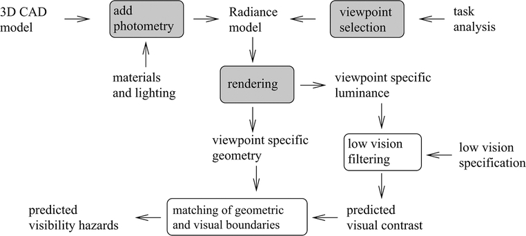
Figure 2 shows the major components of the analysis. Boxes show processing steps. Unboxed text indicates data that is input to and output from these processing steps. The inputs are from 1) a building information modeling system specifying the original architectural design (most of the examples presented here use Revit), 2) additional information about materials and lighting, 3) a task analysis specifying the location and nature of physical mobility hazards and the regions of the architectural space from which they are likely to be viewed, and 4) a low vision specification in terms of either broad categories of visual impairment or specific levels of acuity and contrast sensitivity. System outputs are 1) predicted visual contrast and 2) an indication of predicted visual hazards. A visualization is produced from predicted visual contrast which shows only those environmental features predicted to be visible by an individual with the specified level of visual impairment. The predicted visual hazards can be overlaid on rendered views of the CAD model to warn of physical features that may be difficult or impossible to see under the specified levels of low vision.
Figure 2.
Components of the analysis process. The discovery of hazards to low vision mobility requires many disparate processing steps.
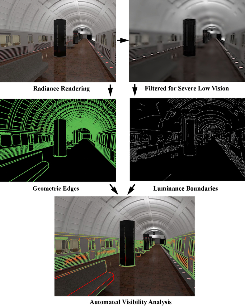
Figure 3 shows an example of the intermediate and final results of the process depicted in Figure 2. The upper left image shows a Radiance rendering of a model of a Washington, DC, subway station. Radiance is one of the few systems available for producing accurate luminance reconstructions of this type. The upper right image shows a version of the upper left image that has been stripped of contrast changes that are predicted to be undetectable by someone with severe low vision. The middle left image marks all of the detected geometry boundaries in the original CAD models with green lines. The middle right image marks all of the predicted luminance boundaries in the low vision image. The bottom image is produced by performing a matching operation on the two middle images. Geometry boundaries are colored using a visualization transfer function with a spectrum ranging from green for boundaries likely to be visible under the specified viewer and environmental conditions, to shades of red for geometric boundaries unlikely to be visible under those conditions. These are the potential visual mobility hazards in the scene.
Figure 3.
A graphical representation of the processing steps.
The processing consists of two main parts. The first converts the original architectural specification into a model suitable for use by the Radiance system for the analysis and visualization of lighting in the design, and then extracts needed information from that model. It involves the gray boxes in Figure 2 and the Rendering, Filtering, and Geometric edges steps in Figure 3. Radiance is used to produce rendered views from the desired viewpoint(s). Importantly, the renderings provide physically correct, photometrically calibrated luminance in a high dynamic range (HDR) format [Grynberg 1989; Ward 1994; Ward & Shakespeare 1998], features not available from most other rendering packages. Radiance is also used to produce viewpoint specific information about model geometry, including position, distance from the viewpoint, and surface orientation over the same grid of pixel points as used for luminance. The second part of the analysis process, shown by the white boxes in Figure 2 and the remainder of Figure 3, starts by applying a computational model of visibility under reduced acuity and contrast sensitivity to the rendered luminance to predict which contrast boundaries will be visible in the view under a particular level of visual impairment [Thompson 2017] and by applying a local discontinuity detection process to the rendered geometry to identify potential mobility hazards. The predicted visibility can then be visualized in two ways: (1) providing the designer with a sense of what the when-built structure would look like under low vision (upper right in Figure 3), or (2) the predicted visibility can be combined with the information about geometric discontinuities, yielding a labeled output showing the presence of potentially hazardous geometric structure unlikely to be visible (reddish lines in lower image in Figure 3).
3. Our System in Action
In our first example, we describe a workflow involving a staircase in the Orlando Lighthouse, a facility dedicated to employing low vision and blind workers, and where many employees have severe low vision. The architect’s REVIT model and specifications were provided and HDR photographs of the stairwell were taken during a site visit after completion. The description is a possible reconstruction of the design process, since our involvement in the project did not start until construction was complete. The building was renovated to add additional workspace for low vision employees and to increase visual accessibility to existing office space by changing lighting and materials. The staircase used in this example is adjacent to the entrance lobby and has considerable use.
One of the limitations in doing research in this area is that it is often difficult to get access to real models. Fortunately, Lighthouse Central Florida and their architects provided access to the remodelled building and models, but after the design was implemented. We looked at the design (specifically the stairway) and reconstructed the kinds of issues that would have occurred during the design process, including materials, lighting, etc. Our goal here is to outline the process as a skilled designer might have approached the project from the beginning.
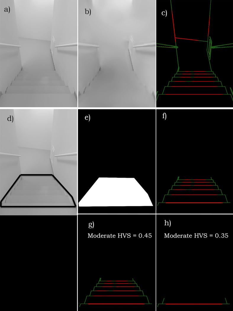
Figure 4a is a rendered view looking down a stairway that is clearly a mobility hazard. Figure 4b is the output of our filtering process applied to this image, with the filter set to represent moderate low vision. The filtered image provides a rough indication of the overall visibility, but such interpretations are subjective and difficult to make in a consistent manner. What is needed is a way to quantify the visibility of specific mobility hazards. To do this, we use an automated analysis to determine an estimate of the visibility. The calculation arises from the assumption that the visibility of a real-world structure is related to how well the visible contours of the object predict the location of actual geometric discontinuities on or bounding the object (Figure 4c), where red lines indicate that the geometry is predicted to be not visible and green lines are predictions of visible geometry. This visualization avoids the need to interpret subtle, localized image changes as to whether or not they correspond to actual scene structure that might pose a mobility hazard. It is, however still hard to interpret because it lacks a holistic characterization of the hazard due to substantial clutter that is not related to mobility impairments. In this particular case a visibility score computed over the whole image has little relevance, since it would include the upper wall edges and features distant from the identified hazard, diluting the score’s relevance. What is needed is a way to quantify the visibility of specific mobility hazards. Our solution involves the designer selecting a Region of Interest (ROI) containing the hazard (Figure 4d), creating an associated mask (Figure 4e) after which the automatic analysis determines an estimate of the visibility of geometrical structure within the ROI (Figure 4f).
Figure 4.
Analysing low-vision visibility from a design model
(a) An HDR computer graphics image of a stairway in the Lighthouse building, modelled with REVIT and rendered with RADIANCE. (b) The original image, filtered to simulate the visibility under moderate low vision. (c) The results of an automated visibility analysis, with red lines indicate geometric structure predicted to not be visible and the green lines indicate geometry predicted to be perceivable. (d) The designer can indicate the boundaries of a portion of the image of particular concern (a region-of-interest (ROI)), which limits where the analysis is performed. (e) Confirmation of the image pixels making up the ROI. (f) Finally, a visualized analysis of the location of mobility hazards, which might be missed if only reviewing the specified conditions of acuity and contrast sensitivity shown in figure b. We show below how to compute a numerical Hazard Visibility Score (HVS) that significantly aids in using this process to choose the optimal design option for the staircase and first step edge (g and h).
Figures 4g and 4h show the results of extending the analysis to produce a quantitative Hazard Visibility Score (HVS) characterizing the predicted visibility of mobility hazards for a particular level of low vision. (Details are provided in the Implementation section). An HVS of 1.0 indicates a prediction of high visibility, lower values are associated with prediction of lower visibility, and an HVS of close to 0.0 indicates that little or no geometric structure is visible. The HVS of 0.45 predicts the staircase hazard as slightly visible at a moderate low vision setting. The HVS of 0.35 for the edge of the first step (Figure 4h) is even lower, an indication of a potentially dangerous hazard. As we will demonstrate, the HVS provides a valuable metric to compare the success of design solutions to improve hazard visibility.
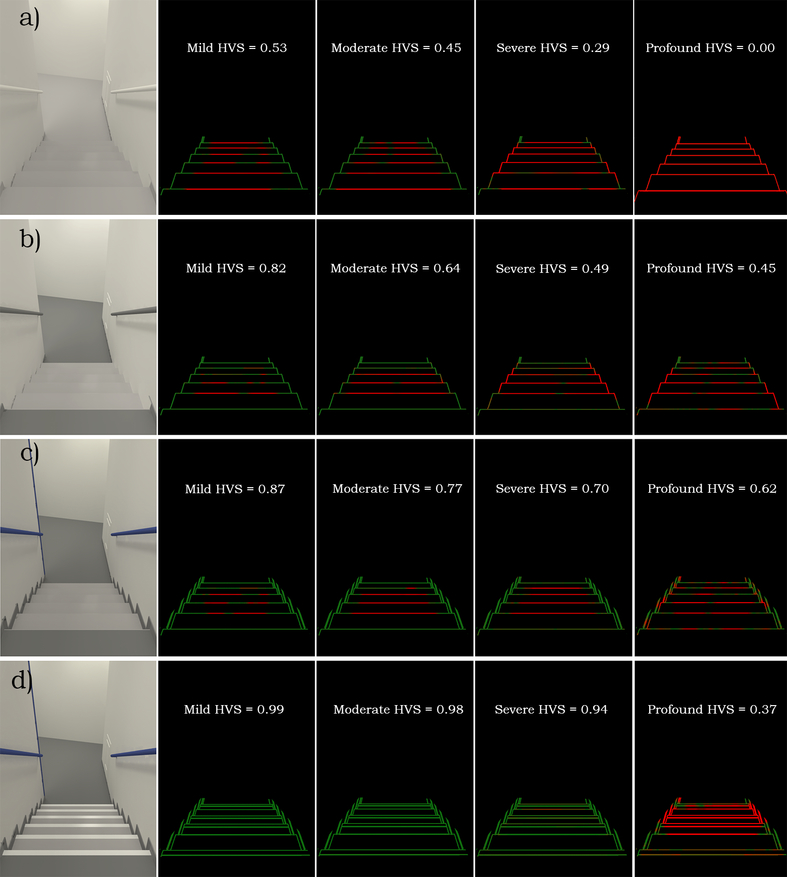
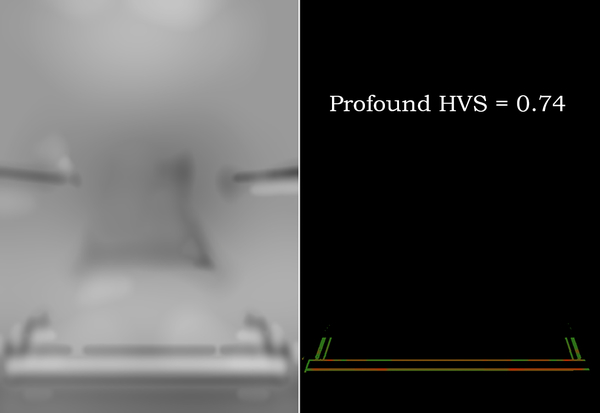
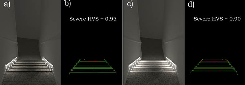
Figures 5a–d present the computed HVS of the same visible portion of the stairway for four low vision settings: mild, moderate, severe, and profound. Note that the analysis for profound (the right-most column in 5a) shows that the hazard is not visible at that level of visual performance. In Figure 5b, the upper and lower floor surfaces were made darker than in Figure 5a. Note the increased visibility of the top and bottom step edges, caused by the increase of contrast between floor and step. The HVS has improved considerably in the mild filtering condition but the other HVSs remain relatively low. Figure 5c shows the effects on visibility of adding baseboards on either side of the stairs. The addition of a white tread grip strip results in the hazard predicted to be visible through severe low vision (Figure 5d). The white strips appear to bloom together under profound low vision, decreasing the HVS. Nevertheless the profound low vision leading edge step has a HVS of 0.74 (Figure 6), significantly more visible than the overall hazard. When comparing the HVS of the designer’s iterative modifications to the original default surface materials, it is clear that the overall visibility of the hazard has been significantly improved. The same model, with overhead lighting turned off, and the addition of carpet and low-level step lighting located on each side of the stairwell, prove to be visually accessible up to severe low vision (Figure 7). Note that the black strips appear to have a slight visibility advantage over the white strips under this lighting condition.
Figure 5.
The computed HVS of the same portion of the stairway for four low vision settings.
(a) Base level (same model as Figure 4).
(b) Upper and lower floor surfaces made darker than (a).
(c) Adding dark baseboards along the sides.
(d) Adding a white tread grip strip.
Figure 6.
Limiting HVS computation to the leading edge of the step.
Figure 7.
Adding night-time lighting and carpet flooring.
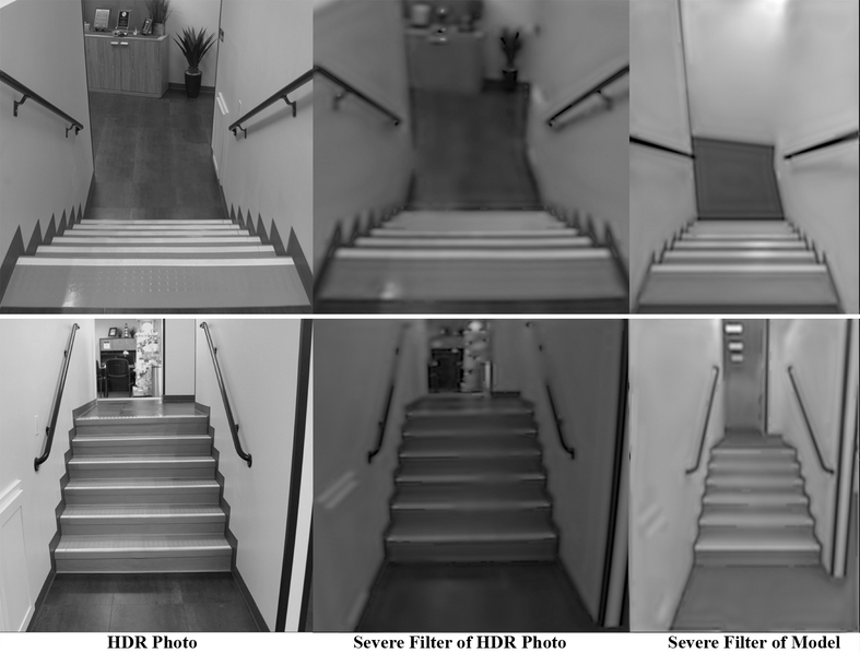
It is possible to apply the low-vision filtering to HDR photographic images in field studies. The resulting images can provide subjective information about the visibility of hazards in a near to completed project. However, while the locations of luminance boundaries could be computed from photographs taken in the field, one would need the corresponding 3D models of the geometry in order to compare the luminance and geometric boundaries. Thus from photographs alone, the automated labeling of low-visibility hazards and the computation of a hazard visibility score (HVS) are not possible. Figure 8 compares an HDR photo of an actual constructed stairwell with severe low vision filtered versions of the real and modeled stairs. Though the realized stairwell was wider than in the REVIT model, the filtered images of the stair treads are highly similar.
Figure 8.
Real stairway (left), photograph of real stairway filtered to simulate severe low vision (center), rendered image of stairway filtered to simulate severe low vision (right).
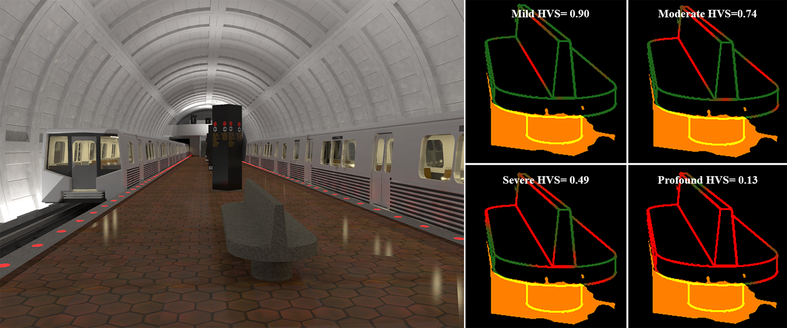
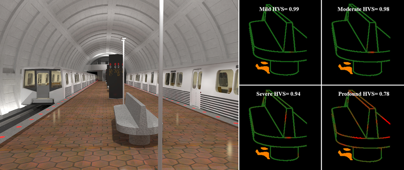
As another example, a complex model of a Washington DC subway station was created from data collected on-site, with the permission of the Washington Metropolitan Area Transit Authority. The model was constructed using Radiance. The low contrast environment was rendered “as is” with the lighting, geometry, and material properties used in the actual station (Figure 9) and then with the addition of virtual area lighting, a reduction in indirect lighting, and a change of bench materials from a low value gray concrete to a whiter granite (Figure 10). HVS values were computed for the region surrounding the bench. Orange is used to mark regions with a luminance below 1 cd/m2. We exclude these regions from the analysis, other than flagging their location, since very low luminance requires special review not yet included in our visibility prediction model. These virtual modifications and the resulting high HVS illustrate the usefulness of automated visibility analysis in exploring and demonstrating an improved design for safe passage for low vision travelers.
Figure 9.
“As is” rendering of subway station with visibility analysis.
Figure 10.
Subway station with exploratory lighting and material changes.
4. An Experiment with Low-Vision Subjects to Test Validity
We conducted an experiment with low-vision subjects to assess the validity of the predictions made by the Hazard Visibility Score (HVS).
Ten low-vision subjects participated. A prior experiment with seven normally sighted subjects with acuity artificially reduced with blur foils to 1.2 logMAR (within the range of our low-vision subjects) demonstrated a significant correlation between performance on our identification task (see below) and the HVS score, providing us with guidance on the size of our participant group. The mean age of our low-vision participants was 46.9 years, range 21 to 66, and there were six males and four females. We recruited the subjects from the roster of University of Minnesota Laboratory for Low-Vision Research. Our primary selection criterion was to recruit subjects with acuities ranging from moderate to profound low vision in the range 0.8 to 1.8 logMAR. We did not impose restrictions based on diagnosis because our computational analysis is not diagnosis specific. We will return to this limitation in the discussion. The resulting sample of subjects had Snellen acuities ranging from 20/126 to 20/914 (0.8 to 1.66 logMAR) measured with the Lighthouse Distance Visual Acuity chart, and contrast sensitivities from 0.2 to 1.65 measured with the Pelli-Robson chart. Primary ocular diagnoses included: three with aniridia, two with retinitis pigmentosa, two with congenital cataract, and one each with glaucoma, optic nerve atrophy, and macular hole. The protocol was approved by the University of Minnesota IRB and each subject signed an IRB-approved consent form.
Testing was conducted in a windowless laboratory room with overhead fluorescent lighting. The seated low-vision subjects viewed a computer display (NEC E243WMi-BK 16:9, 24” widescreen monitor). At the viewing distance of 32 inches, the monitor subtended 34 degrees horizontally and 20 degrees vertically, and was calibrated to produce luminance and contrast values matching those in the simulated test space. The Radiance-generated test images showed a walkway simulating a viewpoint 3.05 m (10 feet) from the architectural feature to be identified. Elsewhere, we have shown good correspondence between the patterns of errors made by observers viewing a real visual environment compared with viewing the same scene on a display matched for local luminance, visual angle, and acuity levels [Carpenter 2018]. While there are advantages to testing viewers in a real-world environment, use of computer-generated images made it feasible to conduct many more test trials and to conveniently vary viewpoint, lighting arrangement and target type.
In each test trial, the computer screen displayed an image containing one of five geometries at the critical location—a large step up 17.8 cm (7 inch) height, a small “tripper” step up 2.54 cm (1 inch), a large step down 17.8 cm (7 inch), a small “tripper” step down 2.54 cm (1 inch) or a flat, uninterrupted continuation of the walkway.
To vary the viewing conditions and the underlying HVS score, the geometries were illuminated by five different lighting arrangements, and by five slightly different viewpoints. In order to ensure that the set of test images would be likely to produce a range of performance above chance guessing and below near-perfect accuracy for the low-vision subjects the images were first tested on normally sighted subjects who wore blurring goggles with Bangerter foils that artificially reduced acuity to average values of 20/316 (1.2 logMAR) and 20/796 (1.6 logMAR) [Odell 2008].
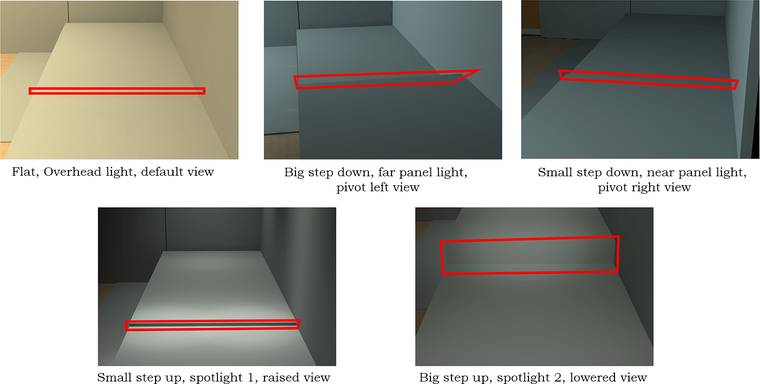
Figure 11 shows 5 examples from the stimuli, sampling five variations in target type, lighting, and viewpoints. Boxes in the figure outline the Regions of Interest (ROIs) used in computing the HVS scores. In total, there were 125 test images (5 geometries x 5 lighting arrangements x 5 viewpoints).
Figure 11.
Five sample images from the stimulus set representing five variations in each design attribute: geometry (flat, large step down, small step down, small step up, large step up), lighting (overhead, far panel, near panel, spotlight 1 and 2), and viewpoint (default, pivot left, pivot right, raised, lowered). The ROI, outlined by a box in each panel, extended 0.5 degrees in visual angle around the step vertices. In the figure, the lines of the box marking ROI boundaries were thickened for clarity.
Each subject was tested twice on each image in randomized order for a total of 250 trials.
Each test image was presented for two seconds. Pilot testing revealed that this duration was long enough for subjects to inspect the display but short enough to permit the entire 250-trial sequence within a two-hour session. Following each image presentation, the low-vision subject indicated verbally which of the five geometries they believed was present. The experimenter recorded the response. The response was scored as correct if the subject accurately reported the geometry in the test image, and incorrect otherwise.
Each of the 125 images was analysed by our hazard visibility software within a region of interest containing the critical geometry. Taking the subject’s acuity and contrast sensitivity into account, an HVS score was computed for each image and each subject. If the HVS score is a valid predictor of feature visibility, we expected to find an association between the probability of our subjects giving the correct response and the HVS scores of the test images. Since the independent variable, HVS, is continuous, and the dependent variable, the subject’s correct or incorrect trial response is binary, we analyzed the data using logistic regression (R software version 3.6.0, function glmer in package lme4, version 1.1–23). The logistic regression tested the relationship between the HVS score and the natural log of the odds by the following formula:
where P is the empirical probability of a correct response, HVS is the Hazard Visibility Score generated by our software, and A and B are slope and intercept parameters of the regression fit.
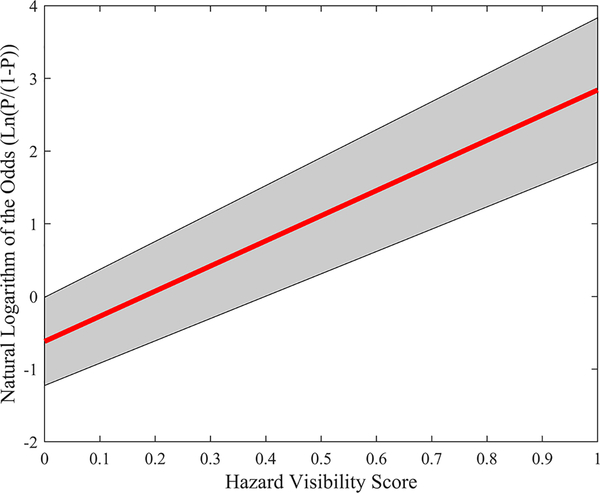
Each subject performed the 250 trials, and HVS scores were computed on a subject-by-subject basis, yielding 2500 trials each with a correct or incorrect outcome and associated HVS value. Figure 12 shows the results of a logistic regression for data aggregated across the 10 subjects. The vertical axis is the logarithm of the odds (Ln(P/(1-P)) and the horizontal axis shows the HVS scores. The fitted logistic regression model is Ln(P/(1-P)) = 3.46*HVS - 0.62 (see Figure 12).
Figure 12.
Visualization of logistic regression model fitted with aggregated data from ten low-vision subjects. The figure plots odds (Ln(P/(1-P)) against HVS. The central line is the fitted regression line, while the gray area marks the confidence interval.
The model shows a significant positive correlation between the odds and HVS. The 95% confidence interval of the slope is (3.07, 3.85), p<.001, indicating that the slope is significantly larger than 0.0. The intercept has a 95% confidence interval of (−1.23, −0.01), p<.05. See Table 2.
Table 2.
The coefficient table for logistic regression model fitted with low-vision subject behavioral testing data.
| Coefficients | Estimate | Standard Error | Z value | P value |
|---|---|---|---|---|
| Intercept (B) | −0.6194 | 0.3093 | −2.002 | 0.0452 |
| Slope (A) | 3.4595 | 0.1971 | 17.548 | 0.2e-16 |
The effect size of a logistic regression model can be represented by its odds ratio (OR), computed as exp(A) where A is the slope. The OR of our fitted logistic regression model is exp(3.46) = 31.8.
When the data were analysed separately for the ten low-vision subjects, all ten individually fitted logistic regression models had slopes significantly greater than zero (p < .05), demonstrating a significant relationship between each subject’s performance and the HVS score.
These empirical results indicate that the HVS score has predictive value in determining the performance of visually impaired subjects in a task involving recognition of 3-D architectural geometry. This finding is a preliminary first step in validating our software. The experiment used only one type of hazard and had a limited sample of low-vision subjects. Future work will be required to validate our software’s prediction of visibility across a wider range of subjects and architectural configurations.
5. Implementation
Architects typically use CAD systems with graphical interfaces, such as REVIT, to construct virtual 3D models. Most of these modeling systems lack the precise photometric simulation capabilities provided by Radiance. Radiance also supports the ability to export local geometric properties such as surface position and surface normal that are registered at the pixel level with luminance. The availability of registered luminance and local geometry is a requirement of our automated visibility analysis workflow. To facilitate integration of our low vision visibility analysis into the typical architect’s work flow, we start by converting REVIT models into a Radiance format using SketchUp Pro with the Open Source Groundhog extension [Groundhog 2017]. (For some of our initial studies, CAD Models of scenes were created directly in Radiance, using a text based, command line interface.) To assure material surfaces are reasonably represented, reflectances are calibrated to closely approximate the characteristics of physical samples of finishes provided by the interior designer and related specifications. Luminaire locations and orientation are similarly checked, adjusted or inserted as indicated on the related Lighting Plan and Luminaire Schedule. Finally, manufacturer supplied luminaire photometric files are referenced to the luminaire locations. This process is similar to the workflow necessary to accurately use many commercial lighting design analysis tools, most of which only generate illumination data, not the photometrically accurate surface luminance calculated by Radiance. The completed Radiance model (geometry, materials, photometry) is then oriented correctly to North in order to integrate accurate daylighting in conjunction with electric lighting. Views, often referred to as virtual camera locations, are located within the model where the scene contains features of potential navigational or hazard interest, such as stairs, ramps, doorways, permanent furnishings and other related architectural features. View heights range from wheelchair eye level to standing eye level 101.6 to 177.8 cm (40” to 70”). The lighting conditions, which might include daylight sequences and day/night time electric light settings, are then determined. The Radiance rendering procedure begins with compiling the scene’s geometry, materials and photometry which is then processed for a viewpoint to render an HDR image. The HDR image, vantage point and metrics required for the visibility analysis phase are extracted.
We have previously reported on a computational model for simulating visibility under varying amounts of reduced acuity and reduced contrast sensitivity [Thompson 2017]. The model uses a non-linear filtering approach adapted from [Peli 1990] to transform a photometrically calibrated input image into a new image in which only image structure above specified acuity and contrast limits is preserved. The goal is not to simulate the subjective experience of viewing the scene under low vision conditions, but rather to produce an image for viewing by those with normal vision in which the only visible features are also visible to those with the specified level of low vision. Low acuity is often simulated by simple blurring. More control over the nature and amount of acuity loss can come from convolving the original image with the desired contrast sensitivity function (CSF). This approach still depends on the visual sensitivity of the user and, even more importantly, is limited in simulating loss of contrast sensitivity. Peli [1990] used a band-pass filtering approach that computes calibrated Michelson contrast for each frequency band. Meaningful thresholding can be applied locally to these bands to remove variability below the visibility limits and then the bands can be reassembled into a single image. [Thompson 2017] extended this approach by making it controllable using the standard measures of acuity and contrast sensitivity. For low vision, this task is complicated by the fact that the clinical measure of acuity references a different portion of the CSF than do the common measures of contrast sensitivity. (See [Peli 1990; Thompson 2017] for more details.) This transformed image can serve as a quick look tool for a designer—if a mobility hazard cannot be seen in the processed image, it is likely a risk to low vision individuals.
Automatic analysis involves comparing the spatial locations of luminance and geometric boundaries. This calculation arises from the assumption that the visibility of a real-world structure is related to how well the visible contours of the object predict the location of actual geometric discontinuities on or bounding the object. We do this by looking over a user specified region of interest covering the actual location of the potential hazard and computing the distance in visual angle between each geometric boundary point and the nearest visible luminance boundary point. Visual acuity is closely related to visual angle. Someone with “normal vision” should be just able to read a high contrast printed character that subtends about 5 arc minutes—move the printed character twice as far from the viewer and it will have to be twice as big to be legible. Since we are evaluating visibility based on acuity, we need to work with angular units.
Luminance boundaries are found by applying the [Canny 1986] edge detector, as modified by [Fleck 1992], to the images generated by the [Thompson 2017] process. Hysteresis thresholding is used, with the high threshold set to include the top 40% of the gradient magnitude values at directional local maxima and the low threshold set to be 0.6 times the high threshold. Gaussian blur pre-smoothing is done using σ = pixels. Because invisible contours are largely removed in our filtered images, edge detection thresholding is less sensitive to parameter setting than is often the case in image processing, but some care is still required. There are no standard methods for estimating the location of geometric boundaries given the information available to us in our models and registered with the luminance data. We have developed two complementary methods that seem to work well (see Appendix), but many other approaches are possible.
Exact co-location of contrast and geometric discontinuities is not required, since the spatial localization of contrast boundaries is typically inexact. However, the amount of fine-scale image structure coincident with localized geometric structure is correlated with a local visibility measure which depends on the distance (measured as a visual angle) to the closest luminance edge from each localized geometric discontinuity. As a result, we compute the distance in visual angle between each point on a geometric boundary and the closest point on any luminance boundary. This closest-point distance, which can be efficiently computed using distance transforms such as described in [Barrow 1977; Felzenszwalb 2012], are used as a measure of the visibility of a geometric feature. Higher value of this measure is an indication that the feature is less likely to be detected under low vision conditions. For visualization purposes, a visualization transfer function is specified by mapping the angular distance to a hazard estimation using magnitude normalization and then a Gaussian weighting function:
| (1) |
| where: | h | = magnitude of hazard |
| dangle | = closest distance in units of visual angle | |
| σh | = scaling parameter (0.75 for all examples presented here) |
Many functions could be used, but the key is that they be smooth, monotonically decreasing, and approach 0.0 for angular distances beyond which a valid correspondence is likely to occur. Currently, the parameters of the transform are set empirically, based on an analysis of test cases marked up with actual geometry features, automatically computed contrast boundaries, and hand drawn locations of feature boundaries. This is fine when the tool is being used by a designer to explore the general visual accessibility of a space and to make choices about materials and illumination. However, substantial calibration will be required before the hazard visibility score can be used as part of a quantitative standard applicable to a wide range of environments.
Since knowing the likelihood of being able to see one point on a potential hazard is of limited value, we average the hazard value over all such points in each analysed image, producing the HVS. Since this equally weights each geometry point in the image, this is most often combined with a region of interest (ROI) specification that limits the computation to the specific areas with mobility hazards of questionable visibility.
All code written for this project is open source and accessible from (https://github.com/visualaccessibility/DeVAS-filter).
6. Discussion
The visibility tool described in this paper provides a proof-of-concept for a design process that uses (1) viewpoint-specific luminance-based analysis and (2) simulations of low vision, to aid in the creation of architectural spaces that are accessible to those with vision impairment. The goals are to provide designers with a tool for enhancing visual accessibility as a part of universal design, and to provide a starting point for luminance-based design standards.
Photometrically accurate renderings of an architectural model have at least a three-decade history, offering the potential for luminance based design, yet with the exception of perhaps the daylighting Roadway and Tunnel Lighting communities [Wienold 2006; Rockcastle 2014; ANSI-IES 2018] luminance studies leading to design choices have not evolved into the architectural design workflow. Current lighting design practice has an essential reliance on metrics which could be reasonably calculated using emerging computing resources available in the 1980’s. Today computing speeds are exponentially faster enabling the viability of luminance based design. A practical approach to predicting what can and what cannot be seen, as part of a design process, has proven elusive, particularly when designing to include visual accessibility for people with low vision.
The design workflow examples we present illustrate a functional step towards designing directly by what should be seen, based on luminance and empirical investigations of low vision. The Lighthouse stairwell sequence, built from an architect’s REVIT model, demonstrates an iterative design process exploring material properties and their shape, resulting in safe visual passage for all but the most severely visually impaired. The stairwell night lighting comparison illustrates a collaborative visibility study between interior design and lighting design. The subway examples focus primarily on the effect of lighting to improve visual accessibility. The key factor used to compare the effectiveness of design choices in each of these examples is the Hazard Visibility Score, which delivers a single metric, a step towards compliance with possible future visibility standards and design practices.
Validating luminance-based design systems is intrinsically more complicated than evaluating illuminance based designs because viewpoint needs to be considered. Adding in considerations of low vision further complicate the effort because of the multiplicity of visual deficits that can occur. However, designers and those formulating safety standards need to accept this extra effort if they want the design to function as intended in the real world. We have provided examples of the sorts of studies needed to calibrate design systems to reflect the needs of people with low vision navigating through potentially hazardous spaces.
Our approach focuses on estimating the visibility of localized hazards, such as steps or benches. Factors in addition to visibility play roles in determining whether a person with low vision can recognize a hazard. For example, a person with severe peripheral field loss may not locate the target within their remaining small field of view (tunnel vision). Eye movements and head orientation will play important roles in determining whether the hazard is seen. In other situations, prior expectations about upcoming hazards and visible cues such as hand rails or barrier posts may alert low-vision pedestrians about an impending hazard, even if the hazard itself is not visible. While recognizing the importance of these additional factors, we have adopted the view that feature visibility is usually a necessary, if not sufficient condition, for safely negotiating hazards.
Our software represents low-vision status in terms of acuity and contrast sensitivity. Acuity is the most widely used metric for vision status. It is used in demographic studies, as an outcome measure in clinical trials, and for statutory purposes. If measures of contrast sensitivity are also available, the performance of the software may be improved. Otherwise, empirically-based estimates of the covariation of contrast sensitivity with acuity are used. Many variables, in addition to acuity and contrast sensitivity, have an impact on low-vision mobility, including color vision, binocular depth cues, light and dark adaptation, and glare susceptibility. We acknowledge that our software does not account for the wide diversity of low-vision conditions encompassed by variations in these variables. We do believe that a measure of visibility based on acuity and contrast sensitivity, mediated by the human contrast sensitivity function, will provide a useful guide for assessing visual accessibility. Future elaboration of the software can build on the same principles.
We have briefly described a preliminary study with human subjects showing that recognition performance for stepping hazards is correlated with our software’s Hazard Visibility Score. Future validation studies and field evaluations need to be done to expand the range of architectural features, viewing conditions and low-vision subjects to fully determine the utility of our software. A major goal of future research will be to fine-tune the software parameters to maximize the validity of the visibility predictions. The parameter settings in the current implementation can undoubtedly be optimized with a broader range of testing but already demonstrate a measure of validity, enhancing our confidence in the general approach. The methods presented here can be used in conjunction with design software to estimate the visibility of key architectural features for people with impaired vision. If more extensive testing with this approach proves to be successful, its measures could be incorporated into design standards to enhance visual accessibility.
Future work includes considerations of glare and field loss. This will be challenging because relatively little is known about how the interactions between low vision and glare or field loss affect the ability to recognize hazards. The method for detecting geometric boundaries needs to be smarter in its analysis of the size and shape of potential hazards. Substantially more human subject data needs to be collected over a broader range of physical structures. Finally, it should be clear that this design approach requires close collaboration between the major design professions that contribute to a successful visual environment and with the specifications of low vision from the vision science community.
Acknowledgments
Lighthouse Central Florida provided site access to photograph the new stairwell and facilitated the assistance of Pete Hall, Associate AIA, WELL AP, the project architect who created the REVIT model. Greg Ward provided help with Radiance issues. Yichen Liu and Rachel Gage provided assistance with testing of human subjects.
Source of Funding
This work was supported by U.S. Department of Health and Human Services, National Institutes of Health, National Eye Institute BRP grant 2 R01 EY017835-06A1. All of the authors received support from this grant.
Biography
William Thompson is a Professor Emeritus in the University of Utah’s School of Computing. Previously, he was on the Computer Science faculty of the University of Minnesota. He holds degrees degree in physics from Brown University and in Computer Science from the University of Southern California. Dr. Thompson’s research lies at the intersection of computer graphics and visual perception, with the dual aims of making computer graphics more effective at conveying information and using computer graphics as an aid in investigating human perception. This is a multi-disciplinary effort involving aspects of computer science, perceptual psychology, and computational vision.
Rob Shakespeare is a lighting designer/consult specializing in dramatic lighting. With expertise in photometrically accurate lighting simulation, he co-authored, Rendering With Radiance: The Art and Science of Lighting Simulation, with Greg Ward. With a rich background in lighting for theatre, his projects, both national and international, include Retail, Commercial, Houses of Worship, Art Galleries, Historic Renovations, Residential, and Public Art Installations. He is Principal Designer for Shakespeare Lighting Design LLC and headed the MFA in Lighting Design at Indiana university. He has been a member of the DeVAS research team for 11 years.
Siyun Liu is a Ph.D. student in the Cognitive and Brain Sciences program of the Psychology department at the University of Minnesota. She has been working in the Minnesota Laboratory for Low-Vision Research since 2017. Her research interests lie in low-vision and navigation. She mainly uses behavioral testing to approach this issue.
Sarah Creem-Regehr is a Professor of Psychology at the University of Utah. She also holds faculty appointments in the School of Computing and the Neuroscience program at the University of Utah. Her research examines how humans perceive, learn, and navigate spaces in natural, virtual, and visually impoverished environments. Her research takes an interdisciplinary approach, combining the study of space perception and spatial cognition with applications in visualization and virtual environments. Her work in computer graphics and virtual environments has contributed to solutions to improve the utility of virtual environment applications by studying human perception and performance.
Daniel Kersten is Professor of Psychology and a member of the graduate faculties in Neuroscience, and Computer Science and Engineering at the University of Minnesota. His research combines computational, behavioral, and brain imaging techniques to understand human visual perception. He is a recipient of the Koffka Medal and is widely recognized for his contributions to Bayesian theories of object perception. Dr. Kersten has published over 100 papers and book chapters, many of which cross traditional disciplinary boundaries. He is currently working on neural mechanisms underlying the perception of human bodies and methods to predict scene visibility in the design of public spaces.
Gordon Legge is a Distinguished McKnight University Professor of Psychology an Neuroscience at the University of Minnesota. He is the director of the Minnesota Laboratory for Low-Vision Research, and a founding member and scientific co-director of the Center for Applied and Translational Sensory Science (CATSS). Legge’s research concerns visual perception with primary emphasis on low vision. Ongoing projects in his lab focus on the roles of vision in reading and mobility, and the impact of impaired vision on visual centers in the brain. He addresses these issues with empirical studies with human volunteers, computational modeling, and brain-imaging (fMRI) methods.
7. Appendix
Finding Geometric Discontinuities
Geometric discontinuities are found using two tests applied to geometric information about the location and orientation of surface points derived from the Radiance model describing the design space. Each test is evaluated over a n by n image patch centered on a pixel of interest, where n is an odd integer ≥ 3. (n = 3 for all examples presented here.) The first test is designed to detect geometric difference associated with occlusion, which often occurs due to surface boundaries of features such as steps and walls that can impede mobility. The presence of occlusion is in part dependent on viewing position. One of the low-level geometric features we have available to the analysis is the length of the line-of-sight ray from the viewing position to every visible surface point in the rendered image. This suggests that occlusion boundaries could be detected by applying an edge detector algorithm to this distance data. However, this does not work well when the lines of sight intersect the surface at a small glancing angle, since the difference in the line of sight distance to adjacent pixels can be large, even in the absence of occlusion boundaries. This problem is address by using a technique less affected by the relationship between the line-of-sight and the orientation of surfaces in the patch. The approach involves determining the average distance between surface points in the patch and a plane passing through the center point of the patch and with an orientation matching the orientation of the modeled surface at the center of the patch:
| (2) |
| where: | docclusion | = geometric difference associated with occlusion at a particular image location |
| m | = n ( (n − 1)/2 ) | |
| P | = three-dimensional model location associated with the line-of-sight corresponding to a particular image location | |
| N | = three-dimensional surface normal corresponding to a particular image location |
and k and l range from to . The value of m is based on the average number of patch points on the occluded surface when the center of the patch is in fact on a surface boundary. Negating the sum and bounding it below by 0 has the effect of making docclusion positive only when the average deviation of position point in the patch and a plane passing through the center point of the patch with an orientation matching the orientation of the modeled surface as the center of the patch is behind the center point location from the perspective of the viewing location. This is based on the fact that surface normals of visible surface points always point towards rather than away from the viewing location. An occlusion discontinuity is presumed to be located anywhere the directional local maxima of docclusion is greater than tocclusion, where tocclusion is an appropriately chosen threshold value (tocclusion = 2 cm for all examples presented here).
The second test is designed to detect surface creases, which often correspond to steps and other orientation change of walking surface, floor-wall boundaries, sharp bends in wall orientation, and the like. This is done by computing the average over the patch of the difference of surface orientations at equal but opposite distances from the patch center:
| (3) |
| where: | dorientation | = geometric difference associated with orientation discontinuities at a particular image location |
| m | = (n + 1)((n − 1)/2) | |
| N | = three-dimensional surface normal corresponding to a particular image location |
and k and l are such that the summation ranges over all distinct pairs of pixel locations in the patch that are at equal but opposite distances from the center pixel. An orientation discontinuity is presumed to be located anywhere a directional local maxima of dorientation is greater than torientation where torientation is an appropriately chosen threshold value (torientation = 20° for all examples presented here).
These thresholds were determined empirically, based on 6 test models. The results were quite stable, suggesting that a more accurate and precise set of thresholds should be easily established.
Footnotes
Disclosure Statement
The authors have no financial interests to declare.
8. References
- [ANSI-IES] American National Standards Institute / Illuminating Engineering Society. 2018. Recommended Practice for Design and Maintenance of Roadway and Parking Facility Lighting. New York (NY): Illuminating Engineering Society. [Google Scholar]
- [ANSI/IES] American National Standards Institute / Illuminating Engineering Society. 2016. ANSI/IES RP-28–16. Lighting and the visual environment for seniors and the low vision population. NEW YORK (NY): The Illuminating Engineering Society. 128 p. [Google Scholar]
- Barrow HG, Tenenbaum JM, Bolles RC, Wolf HC. 1977. Parametric correspondence and chamfer matching: two new techniques for image matching. IJCAI’77 Proc 5th Joint Conf Artif Intel (2) 659–663. [Google Scholar]
- Bourne RRA, et al. Magnitude, temporal trends, and projections of the global prevalence of blindness and distance and near vision impairment: a systematic review and meta-analysis. 2017. Lancet Glob Health. 5(9): PE888–E897. [DOI] [PubMed] [Google Scholar]
- Campbell FW, Robson JG.1968. Application of Fourier analysis to the visibility of gratings. J of Physiol 197(3):551–566. [DOI] [PMC free article] [PubMed] [Google Scholar]
- Canny JF. 1986. A computational approach to edge detection. IEEE Trans Pattern Anal Mach Intell 8:679–698. [PubMed] [Google Scholar]
- Carpenter B (2018). Measuring the Detection of Objects under Simulated Visual Impairment in 3D Rendered Scenes [Ph.D. Thesis, University of Minnesota]. https://conservancy.umn.edu/handle/11299/201710 [Google Scholar]
- Chan T, Friedman DS, Bradley C, Massof R. 2018. Estimates of Incidence and Prevalence of Visual Impairment, Low Vision, and Blindness in the United States. JAMA Ophthalmol 136(1): 12–19. [DOI] [PMC free article] [PubMed] [Google Scholar]
- Colenbrander A 2003. Aspects of vision loss – visual functions and functional vision. Vis Impair Res. 5(3):115–136. [Google Scholar]
- Felzenszwalb PE, Huttenlocher DP. 2012. Distance transforms of sampled functions. Theory of Computing, 8:415–428. [Google Scholar]
- Fleck MF. Some defects in finite-difference edge finders. 1992. 14(3):337–345. IEEE Trans Pa [Google Scholar]
- Groundhog. 2017. Groundhog Lighting. http://www.groundhoglighting.com. Accessed 2018 August 15.
- Grynberg A. 1989. Validation of Radiance, LBID 1575. LBL Technical Information Department Lawrence Berkeley Laboratory. [Google Scholar]
- Ward GJ, Shakespeare RA. 1998. Rendering with Radiance: the art and science of lighting visualization. San Francisco (CA): Morgan Kaufmann Publishers. [Google Scholar]
- [NIBS] National Institute of Building Sciences. 2015. Design Guidelines for the Visual Environment. [Google Scholar]
- Odell NV, Leske DA, Hatt SR, Adams WE, Holmes JM. 2008. The effect of Bangerter filters on optotype acuity, Vernier acuity, and contrast sensitivity. J Aapos 12(6):555–559. [DOI] [PMC free article] [PubMed] [Google Scholar]
- Rea MS. 1986. Toward a Model of Visual Performance: Foundations and Data, J Illum Eng Soc. 15:2, 41–57. [Google Scholar]
- Rea MS, Ouellette MJ.1991. Relative visual performance: A basis for application. Light Res Techno 23(3):135–144. [Google Scholar]
- Peli E 1990. Contrast in complex images. J Opt Soc Am A. 7(10):2032–2040. [DOI] [PubMed] [Google Scholar]
- Rockcastle S and Andersen M. 2014. Measuring the dynamics of contrast & daylight variability in architecture: A proof-of-concept methodology. Build Environ. 81(0):320–333. [Google Scholar]
- Van Den Wymelenberg K and Inanici M. 2015. Evaluating a New Suite of Luminance-Based Design Metrics for Predicting Human Visual Comfort in Offices with Daylight. LEUKOS, 12(3):113–138 [Google Scholar]
- Wienold J, Christoffersen J. 2006. Evaluation methods and development of a new glare prediction model for daylight environments with the use of CCD cameras. Energy and Buildings. 38(7):743–757. [Google Scholar]
- Zaikina V, Matusiak BS and Klöckner CA. 2015. Luminance-Based Measures of Shape and Detail Distinctness of 3D Objects as Important Predictors of Light Modeling Concept. Results of a Full-Scale Study Pairing Proposed Measures with Subjective Responses. LEUKOS, 11(4):193–207. [Google Scholar]
- Ward GJ. 1994. The RADIANCE lighting simulation and rendering system. In Proceedings of the 21st annual conference on computer graphics and interactive techniques. p.459–472. [Google Scholar]
- Thompson WB, Legge GE, Kersten DJ, Shakespeare RA, Lei Q. 2017. Simulating visibility under reduced acuity and contrast sensitivity. J Opt Soc Am A 34(4):583–593. 10.1364/JOSAA.34.000583 [DOI] [PMC free article] [PubMed] [Google Scholar]
- Pelli DG, Robson JG, Wilkins AJ. 1988. The design of a new letter chart for measuring contrast sensitivity. Clin Vision Sci 2:187–199. [Google Scholar]


