Characterizing Protein Protonation Microstates Using Monte Carlo Sampling

Abstract

Proteins are polyelectrolytes with acidic and basic amino acids Asp, Glu, Arg, Lys, and His, making up ≈25% of the residues. The protonation state of residues, cofactors, and ligands defines a “protonation microstate”. In an ensemble of proteins some residues will be ionized and others neutral, leading to a mixture of protonation microstates rather than in a single one as is often assumed. The microstate distribution changes with pH. The protein environment also modifies residue proton affinity so microstate distributions change in different reaction intermediates or as ligands are bound. Particular protonation microstates may be required for function, while others exist simply because there are many states with similar energy. Here, the protonation microstates generated in Monte Carlo sampling in MCCE are characterized in HEW lysozyme as a function of pH and bacterial photosynthetic reaction centers (RCs) in different reaction intermediates. The lowest energy and highest probability microstates are compared. The ΔG, ΔH, and ΔS between the four protonation states of Glu35 and Asp52 in lysozyme are shown to be calculated with reasonable precision. At pH 7 the lysozyme charge ranges from 6 to 10, with 24 accepted protonation microstates, while RCs have ≈50,000. A weighted Pearson correlation analysis shows coupling between residue protonation states in RCs and how they change when the quinone in the Q_B site is reduced. Protonation microstates can be used to define input MD parameters and provide insight into the motion of protons coupled to reactions.

Introduction

Protons are important players in many biochemical processes. They are lost as chemical bonds are made, and many redox reactions are coupled to proton binding. The transmembrane electrochemical gradient, including a ΔpH, provides an essential store of cellular energy. Protons are therefore routinely transferred in and out of protein active sites and across membrane embedded proteins, requiring changes in protonation states along proton transfer pathways as well as at active sites. Drug binding has been shown to modify the protonation states of the protein as well as the drug itself.¹⁻³ Ion binding can be coupled to changes in residue protonation states.^4,5

It has been underappreciated that proteins exist in a distribution of protonation states. An average protein has approximately 25% acidic and basic residues.⁶ Given that a protonation microstate identifies the protonation state of all acidic and basic groups in the molecule, for N titratable groups there are 2^N protonation microstates. Tautomers are microstates with the same net charge but with the protons binding at different sites. There are

1

tautomers with m protons distributed over N binding sites.

It is well established that proteins exist in an ensemble of conformational states. Proteins are large dynamic molecules. With N atoms there are 3N – 6 vibrations ranging from high-frequency vibrations of individual bonds to larger, slower breathing modes of the protein as a whole. Positional changes can be required for function, and they are also inevitable given the low barriers for many motions. Conformational changes modify hydrogen bond patterns, expose buried side chains to the solution, and thus may change site protonation states.

In contrast to the general recognition of conformational substates, there has been little consideration of proteins existing in multiple protonation states. However, even if the structure is fixed there will be a distribution of protonation microstates when residue pK_as are near the pH. The ensemble of protein conformations broadens the distribution of protonation microstates since the residue proton affinity shifts as they sample different environments. Protonation states also change when ligands are bound^2,3 or when redox reactions occur at bound cofactors.^7,8 Proton pumps move protons through membrane embedded proteins as changes in protein conformation and redox states modify residue proton affinity.⁹⁻¹³ As with the protein conformational states, some protonation microstates are essential for protein function while others simply result from multiple microstates being close in energy.

Comparison of Microstates in MD and MC

The ensembles of states generated in any simulation method is limited by the degrees of freedom and the methods of moving between states. In commonly used molecular dynamics (MD) trajectories, atoms and molecules move in time steps, propelled by classical molecular mechanics forces. In standard MD simulations, molecules remain in a single chemical state so their protonation state is fixed at the beginning. Each time step represents a microstate of the system. In Monte Carlo (MC) sampling discrete states are generated based on the chosen degrees of freedom and then retained or rejected based on their energy. States sampled by MC can differ by changing atomic positions, number of atoms, or chemical state including protonation or redox state. An MC microstate thus identifies one choice for all degrees of freedom.

MD trajectories yield large data sets with the molecule moving between many conformations. The challenge is to extract the biological significance of these motions. A fraction of conformational microstates (frames), of the order of 1 in 1000, are saved for analysis. Clustering algorithms group frames to cover the range of diverse conformations based on the similarity score of investigator chosen features. Well-defined clustering approaches include hierarchical clustering (linkage based)^14,15 and center-based clustering (K-means, K-centers).^14,16

We will describe here analysis of protonation microstates obtained with the MCCE program. It uses MC sampling to generate an ensemble of residue and ligand protonation, conformation, and redox states.¹⁷ This is one of a group of programs that calculate the average protonation states for a protein by using grand canonical Monte Carlo sampling (GCMC). They find the probability of each residue being protonated at a given proton chemical potential (pH). Methods include those using semiempirical force fields^18,19 or continuum electrostatics.^20,21 They can have fixed protein positions,^21,22 or include sampling side-chain positions with a rigid backbone as in MCCE. Available software packages for pK_a prediction include MCCE,¹⁷ PROPKA,²³ DelPhiPka,²⁴ H⁺⁺,²⁵ and PypKa.²⁶ The calculation of protonation probability is embedded in MD simulations in cpHMD, allowing simultaneous sampling of protonation and conformational degrees of freedom.²⁷⁻³¹ cpHMD usually uses a classical electrostatic force field with a vacuum dielectric constant but can also use a polarizable force field to obtain a better treatment of the protein dielectric response.³²

Monte Carlo sampling requires consideration of millions of randomly chosen microstates. Traditional calculation of protonation using MC compresses the output to provide only the average probability for the protonation state of each residue at a given pH. A titration is simulated by carrying out the calculation at multiple pHs to derive pK_as for all residues. If other degrees of freedom such as ligand binding or residue conformation are allowed, their probabilities are also found. However, the full microstate distribution contains additional information such as the range of protein net charge and the correlation between protonation of individual sites and with any other available degrees of freedom. Microstate analysis can find the probability of higher energy states that may be reaction intermediates. The protonation microstates can also provide a complete assignment of protonation states for all residues and tautomer states for all His as input for MD. The microstates with the lowest energy or highest probability can be compared.

Here we will describe using grand canonical Monte Carlo within MCCE to characterize the distribution of protonation microstates and their thermodynamic properties using hen white lysozyme and Rb. sphaeroides photosynthetic reaction centers (RCs) as examples. Lysozyme has been used as a test case for pK_a predications, and the protonation probability as a function of pH has been measured.³³⁻³⁶ RCs have a complex network of protonatable residues that function to modulate the electrochemistry of quinone reduction and to serve as a proton transfer pathway to the quinone.^37,38 This larger system will show the complexity of protonation microstates in a system that requires proton transfer for function. The microstate energy distribution, the distribution of microstates with unique charges, the thermodynamics of an individual protonation reaction, and the correlation of the protonation of individual residues will be described.

Methods

The Boltzmann distribution of protonation states and side-chain polar proton positions are found for hen egg white lysozyme (PDB ID: 4lZT(39)) and the reaction centers (RCs) from the purple non-sulfur photosynthetic bacteria Rb. sphaeroides (PDB ID: 1AIG(40)) by using the MCCE program.¹⁷

Conformer Generation Determines the Degrees of Freedom

In MCCE the protein backbone is always fixed. Residue side chains and ligands can be given multiple choices that define their protonation and conformational state. Each choice is a “conformer”. While MCCE can carry out full side-chain rotamer sampling, “isosteric” conformers are used here for simplicity.⁴¹ Key results are shown to be replicated with the more expensive full rotamer search. MCCE can also include explicit waters with multiple positions.⁴² However, as is customary, all water molecules in the crystal structure are deleted and replaced by implicit solvent in lysozyme while 28 crystallographic waters are retained in the RCs, as explicit water molecules play an important role in the proton transfer pathway.^43,44 All protonatable residues (Glu, Asp, Arg, Lys, His, Tyr, and Cys and N- and C-termini) have both charged and neutral conformers available. At each charge state, side-chain conformers are made that differ in the number and position of polar side-chain protons. This includes conformers with protons placed at different positions, such as for different neutral His tautomers and rotation of hydroxyl protons on Tyr, Ser, Thr, and Cys and on neutral Asp and Glu. The ubiquinone in RCs can be oxidized, Q, or anionic semiquinone, Q^•–, in addition to changing the orientation of Asn and Gln amide termini. In the isosteric calculation each residue has from one to ten conformers that are selected in MC sampling. With rotamer search each residue can have from 1 to 118 conformers available.

MCCE Force Field

A microstate of the protein is one selected conformer for each residue. The energy of each microstate is divided into a reference energy plus self- and pairwise interaction energies.¹⁷ The energy of any microstate is obtained from the precalculated energy lookup table. The energy (ΔH^x) of microstate x is

2

The first line describes the energy for each residue type to be in its protonated or unprotonated form or to be oxidized or reduced in solution. Lines two and three describe how the protein shifts the proton and electron affinity of the conformer. M is the total number of conformers. δ_x,i is 1 if conformer i is present in microstate x or 0 otherwise. m_i is 1 for basic protonated, −1 for acidic deprotonated, and 0 for all neutral conformers. pK_sol,i is the reference pK_a of this residue type in solution, and E_m is the reference electrochemical midpoint potential of this redox active group. F is the Faraday constant, and n_i is the change in the number of electrons on a conformer type that is taking part in a redox titration. pH and E_h are the relevant solution parameters describing the chemical potential of protons or electrons that will come to equilibrium with the protein.

The second line of eq 2 describes the self-energies of the conformer that form the microstates. These energies are independent of the conformer choice for other residues. These are the loss of conformer solvation energy as it is moved from the reference solvent to its position in the protein, torsion energy, continuum electrostatic (CE) and Lennard-Jones (LJ) van der Waals interactions with the fixed backbone amides, and favorable van der Waals interactions of the exposed side-chain surface with the implicit solvent.^17,45 The third line gives the continuum electrostatic and Lennard-Jones pairwise interactions between each pair of conformers in other residues. The benchmarks that support the MCCE force field were described previously.¹⁷ All energies are calculated prior to MC sampling. Electrostatic energies are calculated via the Poisson–Boltzmann solver Delphi^20,46,47 using Parse charges⁴⁸ with a dielectric constant of 4 for protein and 80 for solvent and an implicit salt concentration of 150 mM. MCCE corrects the continuum electrostatic energies for the changes in the dielectric boundary due to changes in surface rotamers.¹⁷ Nonelectrostatic energies use the Amber force field.⁴⁹

Monte Carlos Sampling

In MCCE microstates change by random choices, first of a residue and then of a conformer available for that residue. If the chosen residue contains conformers that interact with an absolute value of >0.5 kcal/mol with conformers of another residue, additional conformer changes for that other residue will be made 50% of the time. Here conformers in several residues switch, followed by a single decision using the Metropolis–Hastings algorithm to accept or reject the change. Allowing one to three residues to change helps avoid electrostatic or van der Waals clashes between strongly coupled groups and speeds convergence.^50,51

The Monte Carlo sampling routine starts with a random microstate with one conformer assigned to each residue. The program then goes through annealing, conformer reduction, and MC sampling. Annealing steps down the temperature in the Metropolis–Hastings acceptance criteria. MC sampling is then performed at room temperature. By default, equilibration samples 3000 MC steps/conformer for lysozyme and 300 for RCs. Prior to the production phase, conformers that are rarely chosen are removed from the list of sampled conformers. The default cutoff used here is that a conformer with a probability less than 0.001 is discarded. This speeds convergence and results in acceptance of MC steps of ≈30%. It should be noted that the early elimination of conformers creates problems in highly correlated systems so it can be modified as needed.⁴² The discarded conformers are excluded from all later sampling. If after conformer removal a residue has only a single conformer, then it is a “fixed residue”, which is removed from the sampling list. Free residues have a choice of conformers. A residue whose protonation state becomes fixed by all conformers of one protonation type being discarded may still sample conformers with different positions so it remains on the free residue list.

The total energy is calculated once by using eq 2 for the first random microstate, summing the energy of all chosen conformers. In each subsequent step the interactions with the conformer chosen for change is subtracted from the previous microstate energy and the energy of the new conformer for that residue is added back, speeding the energy calculation. The default number of Monte Carlo steps for the production phase, when microstates are recorded, is 2000 times the number of free conformers. Six independent Monte Carlo cycles of this length starting with a random microstate formed from free conformers are carried out. The six runs are combined, but they can be compared to check the quality of Monte Carlo convergence.

Storage of Monte Carlo Sampling Steps

A major challenge is to record the several million accepted microstates in a readable form. The MCCE algorithm has several features that make this easier. One is that residue conformers are premade and discrete so that we can use the conformer indices as a unique identifier for each microstate. Also, only a few residues are changed on each step so that we need only record the conformers that have changed when a microstate is accepted. Also, no information needs to be updated for fixed residues as they retain their initial conformer selection.

The microstate file starts with a list of conformer IDs that are removed from sampling because they had low probability during preproduction MC sampling and the list of conformers that will be sampled. Likewise, a list of the fixed residues with only one available conformer is separated from the list of free residues that have multiple available conformers. The conformers for the fixed residues are saved at the start. The first line of each MC run gives the initial microstate, listing the occupied conformer ID for all free residues. Subsequent lines record only the conformer IDs that have changed in this step, the microstate energy (kcal/mol), and the microstate count, which is the number of trial microstates that are rejected before the next new microstate is accepted. Links to Jupyter notebooks with tools and tutorials for microstate analysis are found in Supporting Information Link S1.

Generating the Protonation Microstate Ensemble

The microstate file is a ticker tape that must be replayed to find the subsequent microstates. The information can be sorted on many properties. Here we will describe how protonation microstates are identified. Many conformational microstates are aggregated for each unique protonation microstate.

First, the charge of fixed residues that have only a single conformer available in MC is determined. This charge is summed and treated as the background charge which will be added to find the total protein charge in each microstate.

Then the ticker tape is read to place all microstates of free residues into memory. The microstate file gives the conformer ID of each free residue. A simplified microstate is constructed with only the charge of this conformer. This is a vector of the length of all free residues with an entry of −1, 0, or 1 (though groups with other charge states are allowed). Then we determine which charge microstates are unique. The length of the unique microstate vectors is reduced to contain only residues of interest, here acidic and basic residues and the ubiquinone. At each stage the MC count is retained and is summed when multiple conformational microstates are grouped into one protonation microstate.

Correlation between Microstates

Correlation measures the strength of the relationship between two variables with the sign giving the direction of the trend. The weighted Pearson correlation (r_pq),⁵² used here to find residues whose protonation changes are coupled together, is given by

3

Here is the weight, p_i and q_i are the protonation states for two residues in a microstate i, and are the mean value of p_i and q_i respectively, and n is the number of unique accepted charge microstates. The unique charge file is the input. Only those residues whose protonation states take different values in the ensemble are included. The weight of each microstate is the count of accepted microstates that have this unique protonation state. r_pq is calculated for all pairs of residues with variable charge in the microstate ensemble.

Results and Discussion

Traditionally MCCE analysis provides the Boltzmann-averaged protonation and side-chain and ligand position for a protein⁴¹ or other macromolecule.^53,54 The goal is to now characterize the distribution of protonation microstates in the Boltzmann distribution. In MCCE a microstate defines both residue and ligand charge and position. Protonation microstates, which define the charge of every acidic and basic residue, will exist in many conformational states. The charge state identifies the net, total charge in the microstate. Tautomers are groups of protonation microstates that have the same charge but with the protons distributed over different residues.

Microstate Energy Distribution for Lysozyme

Lysozyme is a small protein with 129 residues that is a benchmark protein for pK_a calculations.¹⁷ The 7 Asp, 2 Glu, 1 His, 6 Lys, and N- and C-termini are assigned ionized and neutral conformers. The isosteric conformer routine without explicit waters in MCCE created 284 conformers. Approximately 1–1.5 million microstates are sampled. Considering both protonation and conformation degrees of freedom, 94% of the accepted microstates in Monte Carlo sampling are unique, meaning they are not revisiting a previously accepted microstate.

Figure 1 shows the distribution of microstate energies in the Boltzmann distribution. Even for this small protein, there is a significant energy range. The full width at half-maximum (FWHM) of the skewed normal distribution is 3.61 kcal/mol. There are a small number of microstates at lowest energy, which are well separated from those at highest probability. The shape of the probability distribution is similar at all pHs and for small proteins such as lysozyme and large proteins such as RCs (Figure S1).

Figure 1.

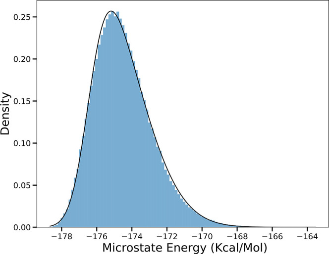
Microstate energy distribution for lysozyme (PDB ID: 4LZT) at pH 7. The density is the probability density, and each bin shows the number of times microstates in that energy window are accepted divided by the total number of accepted microstate and the bin width. Thus, the area under the histogram integrates to 1. The black line is the best fit to a skewed normal distribution curve with a skew of 2.86.

In the lysozyme calculation, at pH 4 there are >500,000 unique accepted conformation/protonation microstates and >200,000 at pH 7. Near the residue pK_a both protonated and deprotonated conformers are in the accepted ensemble. Thus, the number of unique accepted microstates reflects the number of residues that are titrating (Table 1). In lysozyme most residues have pK_as close to their solution values. Thus, at low pH the acids are titrating. At pH 4, ten residues have significant probability of being either charged or neutral, leading to 222 unique protonation microstates. Near pH 7, most Asp and Glu and the C-terminus are stably deprotonated and Lys and Arg protonated. Here, the protonation microstates reflect the mixture of His and N-terminus protonation states (Table S1). At pH 7, only six residues are in a distribution of protonation states, and there are only 24 different protonation microstates in the accepted ensemble (Table 1).

Table 1. Characterization of Accepted Microstates Obtained with Metropolis–Hastings Sampling^a.

	number: all microstates		number: protonation microstates				number: residues
	MC steps	unique accepted (%)	unique	lowest energyb	average energyb	highest energyb	change protonation
pH	lysozyme
4	1,500,000	527,014 (95.4%)	222	4	89	6	10
5	1,500,000	484,152 (94.59%)	147	2	28	2	11
6	1,200,000	430,904 (94.28%)	38	2	15	7	7
7	1,200,000	447,522 (94.72%)	24	4	16	4	6
state	RCs (pH 7)
QB	8,700,000	2,735,799 (99.19%)	60,381	3	24,254	1	53
50:50	8,294,680	2,765,120 (99.19%)	70,713	4	27,775	6	51
QB•–	8,700,000	2,720,450 (99.21%)	54,448	5	22,202	3	48

^aThe MC steps are the aggregate of 2000 times the number of free conformers times six restarts. Unique microstates have different protonation and/or conformation. Protonation microstates differ in location of protons on acidic and basic groups.

^bNumber of unique protonation states within 1.36 kcal/mol of the lowest or highest energy or of ±0.68 kcal/mol of the average energy. There are 27 protonatable residues (Asp, Glu, Arg, His, and Lys) and chain termini in lysozyme and 132 in RCs. The number of residues that change protonation are those that have different charge states in the microstate ensemble. MC sampling for RCs is performed with the ubiquinone in the Q_B site being the neutral quinone, Q_B, or the anionic semiquinone, Q_B^•–, or with the E_h at the E_m for the quinone so there is a 50:50 mixture of the two states.

Distribution of Charge and Tautomer States

Figure 2 shows the distribution of the unique accepted protonation microstates. This mirrors the distribution of charge states that can be found experimentally. However, experimental measurements of protein net charge combine the charge of the protein and of bound ions.⁵⁵⁻⁵⁷ There are 147 unique protonation states accepted by MC sampling for lysozyme at pH 5 and 24 at pH 7. The ensemble average charge is 9.68 at pH 5 and 7.78 at pH 7 (Figure S2). At pH 5 proteins with charge ranging from 7 to 13 are found, though those with charge 9 or 10 are most probable, having the highest count. Each vertical line of dots in Figure 2 is a group of tautomeric states, with the same charge but different proton distributions. In MCCE every unique charge microstate exists in a many tautomer and conformational microstates covering a wide energy range (Figure S3). Larger and more yellow dots in Figure 2 have more underlying conformational states with this distribution of protons.

Figure 2.

Unique tautomer charge distribution for lysozyme at pH (A) 5 and (B) 7. Each point in the scatter plot is a unique protonation microstate. The count gives its acceptance in MC sampling, with high count indicating higher probability. Color and size of points correspond to the range of microstate energies associated with all microstates found for that protonation microstate. Histogram at the top counts the number of tautomers at each charge.

Even a system as small as lysozyme can have a significant number of unique protonation microstates. However, only a small number are found with significant probability in the Boltzmann ensemble. Thus, there are 2¹⁸ possible protonation states, but at pH 7 only six residues have different protonation states in the microstate ensemble. However, of the 2⁶ (64) possible states, only 24 are ever in an accepted microstate. Figure 2 shows there are two microstates at either pH 5 or 7 that have severalfold more occupancy in MC sampling than any others. Table S1 lists all 24 accepted protonation microstates for lysozyme at pH 7 as an example. Only three microstates have a probability greater than 10%, and they sum to 90% of the ensemble. At pH 5, seven states sum to a probability of 90%.

Thermodynamic Parameters for Protonation Reactions from Analysis of the Microstate Ensemble

The changes in the free energy of a reaction determine the proportion of reactants and products at the system at equilibrium (K_eq). The changes in enthalpy and entropy give insight into the nature of what changes in the reaction. Measurements of the equilibrium constant, K_eq, ΔH, and ΔS are common, and there are methods to calculate these parameters from MD trajectories.⁵⁸⁻⁶⁰ However, calculating ΔG, ΔH, and especially ΔS for complex biological molecules often leads to large uncertainty as it can be hard to sample enough states.⁶¹⁻⁶⁵ Here we analyze the accepted microstates in MCCE to determine the thermodynamic properties of the coupled protonation reactions of Glu35 and Asp52 in lysozyme (Figure 3).

Figure 3.

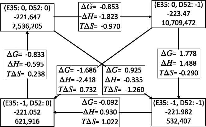
Thermodynamic box for titration of Glu35 and Asp52 in lysozyme at pH 4 at 298.15 K. The full microstate ensemble is sorted into the four protonation states of these two residues, and these groups are independently characterized. Corner boxes: first row is charge of Glu35 and Asp52; second row is the average microstate energy (H); third row is the count of microstates in this protonation state. The boxes along the arrows give the ΔG, ΔH, and TΔS for the transition between different protonation states. The top right and bottom left states are tautomers. All energies are in kcal/mol.

To determine the thermodynamic variables, the MC microstates are divided into four groups, each with a different protonation state for the two residues. ΔH is the difference in average energy reactant and product microstates, given by

4

p counts all product microstates, p_p is the normalized probability and E_p the energy of each, while r counts all reactant microstates, each with probability p_r and energy E_r. The change in free energy is

5

Therefore, the entropy is

6

Additional MC sampling reduces the standard deviation for the calculation of ΔS. Here the numbers of MC steps for annealing and for the production phase are increased 10-fold, with 20,000 steps/conformer performed with the sampling of the free conformers restarted with a new randomly chosen microstate six times.

Figure 3 shows the results for one MCCE calculation at pH 4 where the system is in a mixture of the four protonation microstates. The results for the reaction starting from both acids neutral to both ionized were calculated for 10 independent MC calculations to give values of ΔG of 0.95 ± 0.16 kcal/mol with a ΔH of −0.35 ± 0.02 and −TΔS of 1.30 ± 0.02 kcal/mol. It should be noted that this calculation is performed with a rigid backbone and with limited side-chain flexibility, and so it does not include all changes that will occur in the protein. However, within the constraints of the limited degrees of freedom of the MCCE calculation, thermodynamic variables can be derived from the Boltzmann ensemble with reasonable precision.

Figure 4.

Temperature dependence of thermodynamic parameters. (A) Change in ΔG for the reaction taking Glu35 and Asp52 with both neutral to both ionized with temperature. The line is the linear best fit and each dot represent the ΔG value for an independent MC sampling run using the same input conformer energies. The slope of the graph gives the −ΔS of 0.0045 kcal/(mol deg), and the intercept gives the ΔH of 0.387 kcal/mol; R² is 0.979. (B) Van’t Hoff plot for the same data set. The slope is ΔH/R and intercept ΔS/R, where R is the gas constant. ΔH is 0.377 kcal/mol, and −ΔS is 0.0045 kcal/mol.

An examination of the thermodynamic square shows that the state with Glu35 neutral and Asp52 ionized is favored. This agrees with the ensemble average probability where Glu35 is 8% ionized and Asp52 is 78% ionized, which is in line with the experimental probabilities.³⁴ The breakdown of ΔH and ΔS shows that ΔH plays the larger role, favoring this state.

Thermodynamic Properties with Change in Temperature

The ΔS is traditionally determined from the temperature dependence of a reaction. The same can be done here. The same energy look-up tables are used, but the temperatures of 270, 298.15, 320, and 340 K are used for the Metropolis–Hastings test for microstate acceptance. Ten independent MC calculations are performed at each temperature. All calculated ΔG, ΔH, and ΔS for the system are provided in the Table S3B–D. The standard deviation of the thermodynamic variables is <0.2 kcal/mol, showing the MCCE microstate ensemble can provide reproducible values even for the estimate of ΔS. The same values are obtained from the Van’t Hoff plot of K_eq vs 1/T.⁶² The reaction is exothermic so heat would be released on ionization of the two acids. The standard deviation of the ΔG or K_eq is larger at lower temperatures.

Correlation Analysis of Protonation States of Residues in RCs

A major advantage of having access to the microstates is that the correlation between conformer choices can be found. Here we will describe the correlation of residue protonation states in different microstates using the much larger RCs as an example. It has 828 residues in the coordinate file. There are 132 ionizable residues (Asp, Glu, Arg, Lys, and His) and NTR, CTR, and two redox-active quinones as well as other cofactors. There are 1743 isosteric conformers for the protein, cofactors, and retained water molecules. More than 45 residues are found in a mixture of ionization states at pH 7, and there are more than 50,000 unique protonation microstates to investigate (Table 1).

RCs show the distinction between the lowest energy microstates and those with highest probability. We determined the lowest energy example of each of the 30 most probable protonation microstates (Figure S4). These were compared with the ranking of the microstates at lowest energy. While the high probability states are enriched with lower energy microstates they are not identical. In a thermodynamically equilibrated system states with lower energy, but lower probability, must have lower entropy. The lack of firm alignment of protonation state energy and probability shows that the conformational degrees of freedom are creating more opportunities to make some protonation microstates than others (Figure 2 and Figure S4).

In this system the proton distribution is functionally important as a proton must be brought into the Q_B site, 15 Å from the surface, through a network of protonatable residues and waters.⁶⁶⁻⁶⁸ The Pearson weighted correlation coefficient is used to find the correlation between the residues (eq 3). Residues whose charge state is the same in all microstates are removed from the analysis, as these are not correlated with any other. The weighted correlation coefficient is obtained by taking each unique charge microstates with its corresponding count for the ≈45 remaining residues. Only the residues that have an absolute value of the correlation of at least 0.1 with any other residue are included in the heat map (Figure 5). This procedure identifies 15–16 residues, all of which are near the Q_B site.

Figure 5.

Heat map of Pearson’s weighted correlation coefficient of residue ionization states in RCs at pH 7. Only residues with an absolute value for the correlation ≥0.1 with at least one other residue are shown. Each square in the heat map gives the correlation strength for the two residues obtained with eq 3. Residues are identified as chain (L, M, or H), one letter residue name, and then residue number. Ubiquinone is UQ. Dark blue, blue, sky blue, light gray, orange, red, and dark red correspond to the correlation values in the ranges 0.5 to 1.0, 0.3 to 0.5, 0.1 to 0.3, −0.1 to 0.1, −0.3 to −0.1, −0.5 to −0.3, and −1.0 to −0.5, respectively. (a) Neutral quinone, (b) 50:50 mixture of Q_B and Q_B^•−, and (c) anionic semiquinone Q_B^•–. The quinone is not seen in panel a or c as it is 100% in a single redox state.

The correlation analysis was performed for the RC protonation microstate distribution in three quinone states: neutral quinone, ≈50:50 mixture of the two redox states, and the anionic semiquinone Q_B^•–. A positive correlation indicates that the two groups are more likely to be ionized together, while negative correlation shows that ionization of one reduces ionization of the other. Thus, in the presence of neutral Q_B (Figure 6) the ionization of the group of acidic residues, GluH79, AspL210, GluL212, and AspL213 are negatively correlated to each other. Ionizations of AspM240 and HisH68 are positively correlated. In the presence of Q_B^•– the heat map has two fewer residues than it does in the presence of Q_B. GluL212, which is very close to the quinone, is now always protonated.⁷ As the quinone redox state is expected to modify the protonation states in its vicinity, a heat map is prepared at an E_h where the quinone is ≈50% reduced in the MCCE MC sampling. The protonation of residues that are correlated to the quinone redox state can be seen. Thus, GluL212 and GluL213 are less ionized when the quinone is reduced, while GluH173 and AspL210 are more ionized. Figure 6 shows the position of the residues that are correlated with each other.

Figure 6.

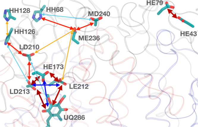
Structure representation of residues that show correlations in the MC sampling with a 50:50 mixture of Q_B and Q_B^•–. Only those residues whose absolute correlation coefficient is ≥0.1 are shown. Residue names follow as chain (L, M, or H), one letter residue name, and then residue number. Ubiquinone is UQ. Blue and red two-sided arrows show the positive and negative correlation, respectively. The color code is the same as Figure 5. Wider arrows indicate a higher correlation.

Conclusions

Proteins have many acidic and basic residues and are very unlikely to be in a single protonation state. Microstate analysis allows us to characterize the ensemble of these states. We have shown that proteins have a range of charge states and for each charge state there are multiple tautomers with a different distribution of protons. While there can be an astonishing number of protonation microstates found in proteins such as RCs, only a few have significant probability. The lower population states may play roles as intermediates in important processes such as proton transfers. The microstate analysis shows how the protonation state of groups of residues are coupled together and which residues are not. The MC ensemble is large enough that the thermodynamic parameters including the ΔS of proton binding can be calculated with reasonable precision.

There are other important properties of proteins whose analysis relies on knowing the microstates rather than simply the average properties. The correlation of structures and protonation state can show how small changes influence the proton affinity of interior sites in the protein.⁶⁹ In proton pumps these changes can lead to efficient proton loading and unloading as protons are transferred through the protein.^12,70 Microstate analysis can show how the protonation states of ligands can shift those of the protein. The proton transfer paths require continuous hydrogen-bonded connections.^71,72 MCCE has been used to find conformers in microstates that make hydrogen bonds in the MC ensemble to trace proton transfer paths.^42,43,73,74 High probability or low-energy microstates that define residue protonation and neutral His tautomers provide rational input to standard MD.

Supporting Information Available

The Supporting Information is available free of charge at https://pubs.acs.org/doi/10.1021/acs.jpcb.2c00139.

• Additional data, figures, and program links (PDF)

The authors declare no competing financial interest.

Special Issue

Published as part of The Journal of Physical Chemistry virtual special issue “Biomolecular Electrostatic Phenomena”.

References

- Intlekofer A. M.; Wang B.; Liu H.; Shah H.; Carmona-Fontaine C.; Rustenburg A. S.; Salah S.; Gunner M. R.; Chodera J. D.; Cross J. R.; Thompson C. B. L-2-Hydroxyglutarate Production Arises from Noncanonical Enzyme Function at Acidic pH. Nat. Chem. Biol. 2017, 13 (5), 494–500. 10.1038/nchembio.2307. [DOI] [PMC free article] [PubMed] [Google Scholar]
- Czodrowski P.; Sotriffer C. A.; Klebe G. Protonation Changes upon Ligand Binding to Trypsin and Thrombin: Structural Interpretation Based on pKa Calculations and ITC Experiments. J. Mol. Biol. 2007, 367 (5), 1347–1356. 10.1016/j.jmb.2007.01.022. [DOI] [PubMed] [Google Scholar]
- Czodrowski P.; Sotriffer C. A.; Klebe G. Atypical Protonation States in the Active Site of HIV-1 Protease: A Computational Study. J. Chem. Inf. Model. 2007, 47 (4), 1590–1598. 10.1021/ci600522c. [DOI] [PubMed] [Google Scholar]
- Song Y.; Gunner M. R. Using Multiconformation Continuum Electrostatics to Compare Chloride Binding Motifs in α-Amylase, Human Serum Albumin, and Omp32. J. Mol. Biol. 2009, 387 (4), 840–856. 10.1016/j.jmb.2009.01.038. [DOI] [PubMed] [Google Scholar]
- Aguilar B.; Anandakrishnan R.; Ruscio J. Z.; Onufriev A. V. Statistics and Physical Origins of pK and Ionization State Changes upon Protein-Ligand Binding. Biophys. J. 2010, 98 (5), 872–880. 10.1016/j.bpj.2009.11.016. [DOI] [PMC free article] [PubMed] [Google Scholar]
- Kim J.; Mao J.; Gunner M. R. Are Acidic and Basic Groups in Buried Proteins Predicted to Be Ionized?. J. Mol. Biol. 2005, 348 (5), 1283–1298. 10.1016/j.jmb.2005.03.051. [DOI] [PubMed] [Google Scholar]
- Okamura M. Y.; Paddock M. L.; Graige M. S.; Feher G. Proton and Electron Transfer in Bacterial Reaction Centers. Biochim. Biophys. Acta 2000, 1458 (1), 148–163. 10.1016/S0005-2728(00)00065-7. [DOI] [PubMed] [Google Scholar]
- Wraight C. A. Chance and Design—Proton Transfer in Water, Channels and Bioenergetic Proteins. Biochim. Biophys. Acta 2006, 1757 (8), 886–912. 10.1016/j.bbabio.2006.06.017. [DOI] [PubMed] [Google Scholar]
- Gunner M. R.; Amin M.; Zhu X.; Lu J. Molecular Mechanisms for Generating Transmembrane Proton Gradients. Biochim. Biophys. Acta 2013, 1827 (8–9), 892–913. 10.1016/j.bbabio.2013.03.001. [DOI] [PMC free article] [PubMed] [Google Scholar]
- Ishikita H.; Saito K. Proton Transfer Reactions and Hydrogen-Bond Networks in Protein Environments. J. Royal Soc. Interface 2014, 11 (91), 20130518–20130519. 10.1098/rsif.2013.0518. [DOI] [PMC free article] [PubMed] [Google Scholar]
- Wikström M.; Sharma V.; Kaila V. R. I.; Hosler J. P.; Hummer G. New Perspectives on Proton Pumping in Cellular Respiration. Chem. Rev. 2015, 115 (5), 2196–2221. 10.1021/cr500448t. [DOI] [PubMed] [Google Scholar]
- Cai X.; Son C. Y.; Mao J.; Kaur D.; Zhang Y.; Khaniya U.; Cui Q.; Gunner M. R. Identifying the Proton Loading Site Cluster in the Ba3 Cytochrome c Oxidase That Loads and Traps Protons. Biochim. Biophys. Acta 2020, 1861 (10), 148239. 10.1016/j.bbabio.2020.148239. [DOI] [PubMed] [Google Scholar]
- Kaur D.; Khaniya U.; Zhang Y.; Gunner M. R. Protein Motifs for Proton Transfers That Build the Transmembrane Proton Gradient. Front. Chem. 2021, 9, 446. 10.3389/fchem.2021.660954. [DOI] [PMC free article] [PubMed] [Google Scholar]
- Shao J.; Tanner S. W.; Thompson N.; Cheatham T. E. Clustering Molecular Dynamics Trajectories: 1. Characterizing the Performance of Different Clustering Algorithms. J. Chem. Theory Comput. 2007, 3 (6), 2312–2334. 10.1021/ct700119m. [DOI] [PubMed] [Google Scholar]
- Husic B. E.; Pande V. S. Ward Clustering Improves Cross-Validated Markov State Models of Protein Folding. J. Chem. Theory Comput 2017, 13 (3), 963–967. 10.1021/acs.jctc.6b01238. [DOI] [PubMed] [Google Scholar]
- Haack F.; Fackeldey K.; Röblitz S.; Scharkoi O.; Weber M.; Schmidt B. Adaptive Spectral Clustering with Application to Tripeptide Conformation Analysis. J. Chem. Phys. 2013, 139 (19), 194110. 10.1063/1.4830409. [DOI] [PubMed] [Google Scholar]
- Song Y.; Mao J.; Gunner M. R. MCCE2: Improving Protein pKa Calculations with Extensive Side Chain Rotamer Sampling. J. Comput. Chem. 2009, 30 (14), 2231–2247. 10.1002/jcc.21222. [DOI] [PMC free article] [PubMed] [Google Scholar]
- Citra M. J. Estimating the pKa of Phenols, Carboxylic Acids and Alcohols from Semi-Empirical Quantum Chemical Methods. Chemosphere 1999, 38 (1), 191–206. 10.1016/S0045-6535(98)00172-6. [DOI] [PubMed] [Google Scholar]
- Tehan B. G.; Lloyd E. J.; Wong M. G.; Pitt W. R.; Montana J. G.; Manallack D. T.; Gancia E. Estimation of pKa Using Semiempirical Molecular Orbital Methods. Part 1: Application to Phenols and Carboxylic Acids. Quant. Struct-Act. Rel. 2002, 21 (5), 457–472. 10.1002/1521-3838(200211)21:5<457::AID-QSAR457>3.0.CO;2-5. [DOI] [Google Scholar]
- Baker N. A. Improving Implicit Solvent Simulations: A Poisson-Centric View. Curr. Opin. Struct. Biol. 2005, 15 (2), 137–143. 10.1016/j.sbi.2005.02.001. [DOI] [PubMed] [Google Scholar]
- Gunner M. R.; Baker N. A. Continuum Electrostatics Approaches to Calculating pKas and Ems in Proteins. Meth. Enzymol. 2016, 578, 1–20. 10.1016/bs.mie.2016.05.052. [DOI] [PMC free article] [PubMed] [Google Scholar]
- Alexov E.; Mehler E. L.; Baker N.; Baptista A.; Huang Y.; Milletti F.; Nielsen J. E.; Farrell D.; Carstensen T.; Olsson M. H. M.; Shen J. K.; Warwicker J.; Williams S.; Word J. M. Progress in the Prediction of pKa Values in Proteins. Proteins 2011, 79 (12), 3260–3275. 10.1002/prot.23189. [DOI] [PMC free article] [PubMed] [Google Scholar]
- Olsson M. H. M.; Søndergaard C. R.; Rostkowski M.; Jensen J. H. PROPKA3: Consistent Treatment of Internal and Surface Residues in Empirical pKa Predictions. J. Chem. Theory Comput. 2011, 7 (2), 525–537. 10.1021/ct100578z. [DOI] [PubMed] [Google Scholar]
- Wang L.; Zhang M.; Alexov E. DelPhiPKa Web Server: Predicting pKa of Proteins, RNAs and DNAs. Bioinformatics 2016, 32 (4), 614–615. 10.1093/bioinformatics/btv607. [DOI] [PMC free article] [PubMed] [Google Scholar]
- Anandakrishnan R.; Aguilar B.; Onufriev A. V. H++ 3.0: Automating pK Prediction and the Preparation of Biomolecular Structures for Atomistic Molecular Modeling and Simulations. Nucleic Acids Res. 2012, 40 (W1), W537–W541. 10.1093/nar/gks375. [DOI] [PMC free article] [PubMed] [Google Scholar]
- Reis P. B. P. S.; Vila-Viçosa D.; Rocchia W.; Machuqueiro M. PypKa: A Flexible Python Module for Poisson–Boltzmann-Based pKa Calculations. J. Chem. Inf. Model. 2020, 60, 4442. 10.1021/acs.jcim.0c00718. [DOI] [PubMed] [Google Scholar]
- Baptista A. M.; Martel P. J.; Petersen S. B. Simulation of Protein Conformational Freedom as a Function of pH: Constant-pH Molecular Dynamics Using Implicit Titration. Proteins 1997, 27 (4), 523–544. 10.1002/(SICI)1097-0134(199704)27:4<523::AID-PROT6>3.0.CO;2-B. [DOI] [PubMed] [Google Scholar]
- Wallace J. A.; Shen J. K. Predicting pKa Values with Continuous Constant pH Molecular Dynamics. Methods Enzymol 2009, 466, 455–475. 10.1016/S0076-6879(09)66019-5. [DOI] [PubMed] [Google Scholar]
- Swails J. M.; York D. M.; Roitberg A. E. Constant pH Replica Exchange Molecular Dynamics in Explicit Solvent Using Discrete Protonation States: Implementation, Testing, and Validation. J. Chem. Theory Comput. 2014, 10 (3), 1341–1352. 10.1021/ct401042b. [DOI] [PMC free article] [PubMed] [Google Scholar]
- Radak B. K.; Chipot C.; Suh D.; Jo S.; Jiang W.; Phillips J. C.; Schulten K.; Roux B. Constant-pH Molecular Dynamics Simulations for Large Biomolecular Systems. J. Chem. Theory Comput. 2017, 13 (12), 5933–5944. 10.1021/acs.jctc.7b00875. [DOI] [PMC free article] [PubMed] [Google Scholar]
- Damjanovic A.; Miller B. T.; Okur A.; Brooks B. R. Reservoir pH Replica Exchange. J. Chem. Phys. 2018, 149 (7), 072321. 10.1063/1.5027413. [DOI] [PMC free article] [PubMed] [Google Scholar]
- Aleksandrov A.; Roux B.; MacKerell A. D. pKa Calculations with the Polarizable Drude Force Field and Poisson–Boltzmann Solvation Model. J. Chem. Theory Comput. 2020, 16 (7), 4655–4668. 10.1021/acs.jctc.0c00111. [DOI] [PMC free article] [PubMed] [Google Scholar]
- Kuramitsu S.; Hamaguchi K. Analysis of the Acid-Base Titration Curve of Hen Lysozyme. J. Biochem 1980, 87 (4), 1215–1219. [PubMed] [Google Scholar]
- Bartik K.; Redfield C.; Dobson C. M. Measurement of the Individual pKa Values of Acidic Residues of Hen and Turkey Lysozymes by Two-Dimensional 1H NMR. Biophys. J. 1994, 66 (4), 1180–1184. 10.1016/S0006-3495(94)80900-2. [DOI] [PMC free article] [PubMed] [Google Scholar]
- Alexov E. G.; Gunner M. R. Incorporating Protein Conformational Flexibility into the Calculation of pH-Dependent Protein Properties. Biophys. J. 1997, 72 (5), 2075–2093. 10.1016/S0006-3495(97)78851-9. [DOI] [PMC free article] [PubMed] [Google Scholar]
- Kuehner D. E.; Engmann J.; Fergg F.; Wernick M.; Blanch H. W.; Prausnitz J. M. Lysozyme Net Charge and Ion Binding in Concentrated Aqueous Electrolyte Solutions. J. Phys. Chem. B 1999, 103 (8), 1368–1374. 10.1021/jp983852i. [DOI] [Google Scholar]
- Paddock M. L.; Rongey S. H.; McPherson P. H.; Juth A.; Feher G.; Okamura M. Y. Pathway of Proton Transfer in Bacterial Reaction Centers: Role of Aspartate-L213 in Proton Transfers Associated with Reduction of Quinone to Dihydroquinone. Biochemistry 1994, 33 (3), 734–745. 10.1021/bi00169a015. [DOI] [PubMed] [Google Scholar]
- Alexov E.; Miksovska J.; Baciou L.; Schiffer M.; Hanson D. K.; Sebban P.; Gunner M. R. Modeling the Effects of Mutations on the Free Energy of the First Electron Transfer from QA– to QB in Photosynthetic Reaction Centers. Biochemistry 2000, 39 (20), 5940–5952. 10.1021/bi9929498. [DOI] [PubMed] [Google Scholar]
- Walsh M. A.; Schneider T. R.; Sieker L. C.; Dauter Z.; Lamzin V. S.; Wilson K. S. Refinement of Triclinic Hen Egg-White Lysozyme at Atomic Resolution. Acta Crystallogr. A 1998, 54 (4), 522–546. 10.1107/S0907444997013656. [DOI] [PubMed] [Google Scholar]
- Stowell M. H.; McPhillips T. M.; Rees D. C.; Soltis S. M.; Abresch E.; Feher G. Light-Induced Structural Changes in Photosynthetic Reaction Center: Implications for Mechanism of Electron-Proton Transfer. Science 1997, 276 (5313), 812–816. 10.1126/science.276.5313.812. [DOI] [PubMed] [Google Scholar]
- Gunner M. R.; Zhu X.; Klein M. C. MCCE Analysis of the pKas of Introduced Buried Acids and Bases in Staphylococcal Nuclease. Proteins 2011, 79 (12), 3306–3319. 10.1002/prot.23124. [DOI] [PubMed] [Google Scholar]
- Zhang Y.; Haider K.; Kaur D.; Ngo V. A.; Cai X.; Mao J.; Khaniya U.; Zhu X.; Noskov S.; Lazaridis T.; Gunner M. R. Characterizing the Water Wire in the Gramicidin Channel Found by Monte Carlo Sampling Using Continuum Electrostatics and in Molecular Dynamics Trajectories with Conventional or Polarizable Force Fields. J. Comput. Biophys. Chem. 2021, 20 (02), 111–130. 10.1142/S2737416520420016. [DOI] [Google Scholar]
- Kaur D.; Zhang Y.; Reiss K. M.; Mandal M.; Brudvig G. W.; Batista V. S.; Gunner M. R. Proton Exit Pathways Surrounding the Oxygen Evolving Complex of Photosystem II. Biochim. Biophys. Acta 2021, 1862 (8), 148446. 10.1016/j.bbabio.2021.148446. [DOI] [PubMed] [Google Scholar]
- Wei R.; Zhang Y.; Mao J.; Matta D.; Khaniya U.; Gunner M. Comparison of Proton Transfer Paths to the QA and QB Sites of the Rb. sphaeroides Photosynthetic Reaction Centers. bioRxiv 2022, 10, 479886. [DOI] [PubMed] [Google Scholar]
- Levy R. M.; Zhang L. Y.; Gallicchio E.; Felts A. K. On the Nonpolar Hydration Free Energy of Proteins: Surface Area and Continuum Solvent Models for the Solute-Solvent Interaction Energy. J. Am. Chem. Soc. 2003, 125 (31), 9523–9530. 10.1021/ja029833a. [DOI] [PubMed] [Google Scholar]
- Warwicker J.; Watson H. C. Calculation of the Electric Potential in the Active Site Cleft Due to α-Helix Dipoles. J. Mol. Biol. 1982, 157 (4), 671–679. 10.1016/0022-2836(82)90505-8. [DOI] [PubMed] [Google Scholar]
- Rocchia W.; Alexov E.; Honig B. Extending the Applicability of the Nonlinear Poisson–Boltzmann Equation: Multiple Dielectric Constants and Multivalent Ions. J. Phys. Chem. B 2001, 105 (28), 6507–6514. 10.1021/jp010454y. [DOI] [Google Scholar]
- Sitkoff D.; Sharp K. A.; Honig B. Accurate Calculation of Hydration Free Energies Using Macroscopic Solvent Models. J. Phys. Chem. 1994, 98 (7), 1978–1988. 10.1021/j100058a043. [DOI] [Google Scholar]
- Cornell W. D.; Cieplak P.; Bayly C. I.; Gould I. R.; Merz K. M.; Ferguson D. M.; Spellmeyer D. C.; Fox T.; Caldwell J. W.; Kollman P. A. A Second Generation Force Field for the Simulation of Proteins, Nucleic Acids, and Organic Molecules. J. Am. Chem. Soc. 1995, 117 (19), 5179–5197. 10.1021/ja00124a002. [DOI] [Google Scholar]
- Beroza P.; Fredkin D. R.; Okamura M. Y.; Feher G. Protonation of Interacting Residues in a Protein by a Monte Carlo Method: Application to Lysozyme and the Photosynthetic Reaction Center of Rhodobacter Sphaeroides. Proc. Natl. Acad. Sci. U. S. A. 1991, 88 (13), 5804–5808. 10.1073/pnas.88.13.5804. [DOI] [PMC free article] [PubMed] [Google Scholar]
- Yang A. S.; Gunner M. R.; Sampogna R.; Sharp K.; Honig B. On the Calculation of pKas in Proteins. Proteins 1993, 15 (3), 252–265. 10.1002/prot.340150304. [DOI] [PubMed] [Google Scholar]
- Liu Y.; Meng Q.; Chen R.; Wang J.; Jiang S.; Hu Y. A New Method to Evaluate the Similarity of Chromatographic Fingerprints: Weighted Pearson Product-Moment Correlation Coefficient. J. Chromatogr. Sci. 2004, 42 (10), 545–550. 10.1093/chromsci/42.10.545. [DOI] [PubMed] [Google Scholar]
- Frick D. N.; Rypma R. S.; Lam A. M. I.; Frenz C. M. Electrostatic Analysis of the Hepatitis C Virus NS3 Helicase Reveals Both Active and Allosteric Site Locations. Nucleic Acids Res. 2004, 32 (18), 5519–5528. 10.1093/nar/gkh891. [DOI] [PMC free article] [PubMed] [Google Scholar]
- Hong J.; Hamers R. J.; Pedersen J. A.; Cui Q. A Hybrid Molecular Dynamics/Multiconformer Continuum Electrostatics (MD/MCCE) Approach for the Determination of Surface Charge of Nanomaterials. J. Phys. Chem. C 2017, 121 (6), 3584–3596. 10.1021/acs.jpcc.6b11537. [DOI] [Google Scholar]
- Durant J. A.; Chen C.; Laue T. M.; Moody T. P.; Allison S. A. Use of T4 Lysozyme Charge Mutants to Examine Electrophoretic Models. Biophys. Chem. 2002, 101–102, 593–609. 10.1016/S0301-4622(02)00168-0. [DOI] [PubMed] [Google Scholar]
- Moody T. P.; Kingsbury J. S.; Durant J. A.; Wilson T. J.; Chase S. F.; Laue T. M. Valence and Anion Binding of Bovine Ribonuclease A between PH 6 and 8. Anal. Biochem. 2005, 336 (2), 243–252. 10.1016/j.ab.2004.09.009. [DOI] [PubMed] [Google Scholar]
- Laue T. Charge Matters. Biophys. Rev. 2016, 8 (4), 287–289. 10.1007/s12551-016-0229-3. [DOI] [PMC free article] [PubMed] [Google Scholar]
- Levy R. M.; Gallicchio E. Computer Simulations with Explicit Solvent: Recent Progress in the Thermodynamic Decomposition of Free Energies and in Modeling Electrostatic Effects. Annu. Rev. Phys. Chem. 1998, 49 (1), 531–567. 10.1146/annurev.physchem.49.1.531. [DOI] [PubMed] [Google Scholar]
- Ahmad M.; Helms V.; Lengauer T.; Kalinina O. V. Enthalpy–Entropy Compensation upon Molecular Conformational Changes. J. Chem. Theory Comput. 2015, 11 (4), 1410–1418. 10.1021/ct501161t. [DOI] [PubMed] [Google Scholar]
- Chen L.; Cruz A.; Roe D. R.; Simmonett A. C.; Wickstrom L.; Deng N.; Kurtzman T. Thermodynamic Decomposition of Solvation Free Energies with Particle Mesh Ewald and Long-Range Lennard-Jones Interactions in Grid Inhomogeneous Solvation Theory. J. Chem. Theory Comput. 2021, 17 (5), 2714–2724. 10.1021/acs.jctc.0c01185. [DOI] [PMC free article] [PubMed] [Google Scholar]
- Peter C.; Oostenbrink C.; van Dorp A.; van Gunsteren W. F. Estimating Entropies from Molecular Dynamics Simulations. J. Chem. Phys. 2004, 120 (6), 2652–2661. 10.1063/1.1636153. [DOI] [PubMed] [Google Scholar]
- Zhukov A.; Karlsson R. Statistical Aspects of van’t Hoff Analysis: A Simulation Study. J. Mol. Recognit. 2007, 20 (5), 379–385. 10.1002/jmr.845. [DOI] [PubMed] [Google Scholar]
- Ross G. A.; Bodnarchuk M. S.; Essex J. W. Water Sites, Networks, and Free Energies with Grand Canonical Monte Carlo. J. Am. Chem. Soc. 2015, 137 (47), 14930–14943. 10.1021/jacs.5b07940. [DOI] [PubMed] [Google Scholar]
- Ross G. A.; Bruce Macdonald H. E.; Cave-Ayland C.; Cabedo Martinez A. I.; Essex J. W. Replica-Exchange and Standard State Binding Free Energies with Grand Canonical Monte Carlo. J. Chem. Theory Comput. 2017, 13 (12), 6373–6381. 10.1021/acs.jctc.7b00738. [DOI] [PMC free article] [PubMed] [Google Scholar]
- Khrapunov S. The Enthalpy-Entropy Compensation Phenomenon. Limitations for the Use of Some Basic Thermodynamic Equations. Curr. Protein Pept. Sci. 2018, 19 (11), 1088–1091. 10.2174/1389203719666180521092615. [DOI] [PMC free article] [PubMed] [Google Scholar]
- Okamura M. Y.; Feher G. Proton Transfer in Reaction Centers from Photosynthetic Bacteria. Annu. Rev. Biochem. 1992, 61, 861–896. 10.1146/annurev.bi.61.070192.004241. [DOI] [PubMed] [Google Scholar]
- Abresch E. C.; Paddock M. L.; Stowell M. H. B.; McPhillips T. M.; Axelrod H. L.; Soltis S. M.; Rees D. C.; Okamura M. Y.; Feher G. Identification of Proton Transfer Pathways in the X-Ray Crystal Structure of the Bacterial Reaction Center from Rhodobacter sphaeroides. Photosynth. Res. 1998, 55 (2), 119–125. 10.1023/A:1006047519260. [DOI] [Google Scholar]
- Krammer E.-M.; Till M. S.; Sebban P.; Ullmann G. M. Proton-Transfer Pathways in Photosynthetic Reaction Centers Analyzed by Profile Hidden Markov Models and Network Calculations. J. Mol. Biol. 2009, 388 (3), 631–643. 10.1016/j.jmb.2009.03.020. [DOI] [PubMed] [Google Scholar]
- Di Luca A.; Gamiz-Hernandez A. P.; Kaila V. R. I. Symmetry-Related Proton Transfer Pathways in Respiratory Complex I. Proc. Natl. Acad. Sci. U. S. A. 2017, 114 (31), E6314–E6321. 10.1073/pnas.1706278114. [DOI] [PMC free article] [PubMed] [Google Scholar]
- Chenal C.; Gunner M. R. Two Cl Ions and a Glu Compete for a Helix Cage in the CLC Proton/Cl- Antiporter. Biophys. J. 2017, 113 (5), 1025–1036. 10.1016/j.bpj.2017.07.025. [DOI] [PMC free article] [PubMed] [Google Scholar]
- Miyake T.; Rolandi M. Grotthuss Mechanisms: From Proton Transport in Proton Wires to Bioprotonic Devices. J. Phys.: Condens. Matter 2016, 28 (2), 023001. 10.1088/0953-8984/28/2/023001. [DOI] [PubMed] [Google Scholar]
- Siemers M.; Lazaratos M.; Karathanou K.; Guerra F.; Brown L. S.; Bondar A.-N. Bridge: A Graph-Based Algorithm to Analyze Dynamic H-Bond Networks in Membrane Proteins. J. Chem. Theory Comput. 2019, 15 (12), 6781–6798. 10.1021/acs.jctc.9b00697. [DOI] [PubMed] [Google Scholar]
- Cai X.; Haider K.; Lu J.; Radic S.; Son C. Y.; Cui Q.; Gunner M. R. Network Analysis of a Proposed Exit Pathway for Protons to the P-Side of Cytochrome c Oxidase. Biochim. Biophys. Acta 2018, 1859 (10), 997–1005. 10.1016/j.bbabio.2018.05.010. [DOI] [PubMed] [Google Scholar]
- Khaniya U.; Gupta C.; Cai X.; Mao J.; Kaur D.; Zhang Y.; Singharoy A.; Gunner M. R. Hydrogen Bond Network Analysis Reveals the Pathway for the Proton Transfer in the E-Channel of T. Thermophilus Complex I. Biochim. Biophys. Acta 2020, 1861 (10), 148240. 10.1016/j.bbabio.2020.148240. [DOI] [PubMed] [Google Scholar]
Associated Data
This section collects any data citations, data availability statements, or supplementary materials included in this article.