(TAML)Fe^IV═O Complex in Aqueous Solution: Synthesis and Spectroscopic and Computational Characterization

Abstract

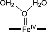
Recently, we reported the characterization of the S = ½ complex [Fe^V(O)B*]⁻, where B* belongs to a family of tetraamido macrocyclic ligands (TAMLs) whose iron complexes activate peroxides for environmentally useful applications. The corresponding one-electron reduced species, [Fe^IV(O)B*]²⁻ (2), has now been prepared in >95% yield in aqueous solution at pH > 12 by oxidation of [Fe^III(H₂O)B*]⁻ (1), with tert-butyl hydroperoxide. At room temperature, the monomeric species 2 is in a reversible, pH-dependent equilibrium with dimeric species [B*Fe^IV–O–Fe^IVB*]²⁻ (3), with a pK_a near 10. In zero field, the Mössbauer spectrum of 2 exhibits a quadrupole doublet with ΔE_Q = 3.95(3) mm/s and δ = −0.19(2) mm/s, parameters consistent with a S = 1 Fe^IV state. Studies in applied magnetic fields yielded the zero-field splitting parameter D = 24(3) cm⁻¹ together with the magnetic hyperfine tensor A/g_nβ_n = (−27, −27, +2) T. Fe K-edge EXAFS analysis of 2 shows a scatterer at 1.69 (2) Å, a distance consistent with a Fe^IV═O bond. DFT calculations for [Fe^IV(O)B*]²⁻ reproduce the experimental data quite well. Further significant improvement was achieved by introducing hydrogen bonding of the axial oxygen with two solvent–water molecules. It is shown, using DFT, that the ⁵⁷Fe hyperfine parameters of complex 2 give evidence for strong electron donation from B* to iron.

1. Introduction

Fe–TAML catalysts (TAML = tetraamido macrocyclic ligand) comprise a family of iron complexes that can activate peroxides to carry out oxidation processes that promise significant environmental impact. To date, they have been demonstrated to be useful, among other things, for destroying trace pollutants in water associated with the textile, pulp and paper, and pesticides industries, for rapidly killing anthraxlike spores and removing sulfur from hydrocarbon fuels.^1,2 The usefulness of Fe–TAML catalysts in a number of practical applications has stimulated us to investigate the chemical basis for their oxidative reactivity.

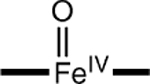
Because their oxidative potency resembles those of oxygen-activating iron enzymes,³ it is not surprising that high-valent iron–oxo species immediately come to mind as putative oxidants for Fe–TAML action. Although TAMLs had been shown to support the iron(IV) oxidation state as early as 1990 (reviewed in ref 4), no definitive evidence for iron–oxo species in the TAML family existed until quite recently. The first breakthrough was the crystallographic characterization of two oxo-bridged diiron(IV) complexes that derived from the reaction of dioxygen with their iron(III) precursors in dichloromethane.⁵ A second significant achievement was the generation of the first example of an oxo–iron(V) complex, [Fe^V(O)B*]⁻ (see Figure 1 for the structure of B*), which was obtained in nearly quantitative yield from the reaction of the [Fe^III(H₂O)B*]⁻, 1, precursor with peracid in butyronitrile at −60 °C. Under these conditions, [Fe^V(O)B*]⁻ persisted for hours and was characterized by UV–vis, Mössbauer, EPR, and X-ray absorption spectroscopies.⁶

Figure 1.

Structures of TAMLs: (A) H₄B* (R = −CH₃, X = −H); H₄DCB (R = −CH₂CH₃, X = −Cl); H₄DMOB (R = −CH₂CH₃, X = −OCH₃) and (B) H₄MAC*. Iron complexes with various axial ligands: (C) [Fe^III(H₂O)B*]⁻ (1), (D) [Fe^IV(O)(NCMe)TMC]²⁺, and (E) [Fe^IV(O)TMCS]²⁺.

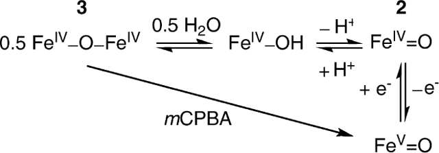
The iron in [Fe^V(O)B*]⁻ has a penta-valent oxidation state, unlike compounds I of cytochrome P450 and the heme peroxidases, which are best described as iron(IV)–radical species.⁷ To obtain the compound II analogue, we have turned our attention to the characterization of a species that is present in the room-temperature oxidation chemistry of aqueous Fe^III–TAML complexes at high pH. Here, we report the generation of a highly stable S = 1 [Fe^IV(O)B*]²⁻, 2, complex, produced in nearly quantitative yield by reacting 1 with tert-butyl hydroperoxide (TBHP) at pH > 12. We have characterized this complex by UV–vis, Mössbauer, and X-ray absorption (XAS) spectroscopies, as well as density functional theory (DFT) calculations. Upon lowering the pH below 12, the Fe^IV═O complex was reversibly transformed into the [B*Fe^IV–O–Fe^IVB*]²⁻ dimer, 3. We thus can describe a series of three high-valent iron–oxo complexes of B* that are inter-related by either one-electron transfer or monomer–dimer reversibility.

The electronic structure of S = 1 Fe^IV═O species has been the subject of extensive spectroscopic and computational, notably DFT, studies.^8–16 The picture emerging from these efforts is that the two odd electrons of Fe^IV are in d_xz and d_yz orbitals that are substantially admixed with the p_x and p_y orbitals of oxygen. The large spin density at oxygen, resulting from the strong d_π–p_π interactions, was confirmed by ¹⁷O ENDOR of compound I of horseradish peroxidase,^8,9 which is an EPR active S = ½ species because of the antiferromagnetic exchange coupling of the Fe═O moiety to the porphyrin cation radical. An alternative description of the Fe═O bond has been proposed by Girerd and co-workers:¹⁷ on the basis of CASSCF calculations, the Fe═O fragment is formulated as a highly correlated iron(III)–oxyl species. DFT has proven to be a useful tool for predicting the zero-field splitting and hyperfine parameters of high-valent iron complexes.^13,18–20 In this study, this computational technique is applied for identifying 2 as a S = 1 Fe^IV═O species and elucidating the influence of the strong donor capacity of TAML on the electronic structure parameters obtained from Mössbauer analysis.

2. Materials and Methods

List of Acronyms for Ligands.

TMC, 1,4,8,11-tetramethyl-1,4,8,11-tetraaza-cyclotetradecane; TMCS, 2-(4,8,11-trimethyl-1,4,8,11-tetraaza-cyclotetradec-1-yl)-ethanethiol; H₄DCB, 2,3-dichloro-10,10-diethyl-7,7,13,13-tetramethyl-5,7,8,12,13,15-hexahydro-5,8,12,15-tetraaza-benzocyclotridecene-6,9,11,14-tetraone; H₄DMOB, 10,10-diethyl-2,3-dimethoxy-7,7,13,13-tetramethyl-5,7,8,12,13,15-hexahydro-5,8,12,15-tetraaza-benzocyclotridecene-6,9,11,14-tetraone; H₄MAC*, 6,6-diethyl-3,3,9,9,12,12,14,14-octamethyl-1,4,8,11-tetraaza-cyclotetradecane-2,5,7,10,13-pentaone; and H₄B*, 7,7,10, 10,13,13-hexamethyl-5,7,8,12,13,15-hexahydro-5,8,12,15-tetraaza-benzocyclotridecene-6,9,11,14-tetraone.

Materials.

All reagents and solvents were purchased from commercial sources and were used as received, unless noted otherwise. The synthesis of Fe–TAML complexes has been described earlier.²¹

Preparation of Samples for Figure 5.

Figure 5.

Solid lines show the change in UV–vis spectral pattern in changing the pH from 8.6 to 13 (solid arrow). Dashed lines show transformation of 2 to 3 as the pH is changed from 13 to 8.6 (see the Materials and Methods).

Samples for Figure 5 were prepared in two sets. First, 0.5 equiv of TBHP (70% aqueous solution) was added to a 1 mM solution of 1 (as the Na salt) prepared in pH 13 buffer (0.01 M phosphate) to obtain 2. A total of 100 μL of this solution was added to each of two separate 900 μL buffered solutions of pH 13 and 8.6. Electronic absorption spectra were recorded until a stable absorbance was obtained (dashed lines). In the second set, 0.5 equiv of TBHP were added to a 1 mM solution of 1 prepared at pH 8.6 to obtain 3. A total of 100 μL of this solution was added to each of two 900 μL buffered solutions of pH 8.6 and 13. Spectra were recorded until a stable absorbance was obtained (solid lines). The spectrum assigned to 3 in Figure 5 differs from that reported in refs 5 and 7. The difference is probably due to the fact that, in this study, 3 was synthesized in water but only to a considerable purity (~ 80%), leaving some residual absorbance of 1 in the 365–400 nm region of Figure 5. The electronic absorption spectrum of 1 is strongly dependent upon pH and has a band at 365 nm that vanishes at pH > 12, making the UV spectral region less suitable for the analysis of the dimer–monomer conversion. Furthermore, the change in solvent may also have played some role in terms of the extinction coefficient.

Preparation of Samples for Mössbauer and XAS Studies.

A typical preparation of ⁵⁷Fe-enriched complex 2 was performed as follows. A 0.5–1 mL solution of ⁵⁷Fe-enriched 1 (1–2 mM) in 1 M KOH solution was placed into an optical cuvette at room temperature. A half equiv of TBHP solution was added and mixed promptly. The reaction was followed by UV–vis spectrometry until the 435 nm band reached a maximum, indicating the complete formation of 2. Solutions were taken out directly from the UV–vis cuvettes to Mössbauer/EXAFS cups and frozen in liquid nitrogen.

Preparation of Samples for Figure 7.

Figure 7.

Plot of the absorbance at 765 and 1050 nm, bands assigned to [B*Fe^IV–O–Fe^IVB*]²⁻, as a function of pH (see the Materials and Methods).

First, a stock solution of 1 (1 mM) was prepared in water. Each time 100 μL of this solution was then added to 900 μL of 0.01 M phosphate buffer of pH 8.6, 9.0, 9.5, 10.0, 10.5, 11.0, 11.5, and 12.0, respectively. The accuracy of the pH measurements was ±0.1 units. To each of these 0.1 mM solutions of 1, 0.5 equiv of TBHP was added and electronic absorption spectra were recorded until a steady absorbance was reached (10–15 min).

Spectroscopy.

UV–vis spectrophotometric measurements were performed using a Hewlett-Packard diode array spectrophotometer (model 8453) equipped with a thermostatted cell holder and an automated 8-cell positioner. A thermo digital temperature controller RTE17 was employed to control the temperature to within an accuracy of ±1 °C. Both quartz and appropriate plastic cuvettes of different path lengths were used.

Mössbauer spectra were recorded with two spectrometers using Janis Research, Inc., SuperVaritemp dewars that allow studies in applied magnetic fields up to 8.0 T in the temperature range from 1.5 to 200 K. Spectral simulations were performed using the WMOSS software package (WEB Research, Minneapolis, MN). Isomer shifts are quoted relative to Fe metal at 298 K.

XAS Analysis of [Fe^IV(O)B*]²⁻.

Fe K-edge X-ray absorption spectra (XAS, fluorescence excitation, Ge detector) were recorded on frozen aqueous solutions at 10(1) K over the energy range of 6.9–8.0 keV. The monochromator was calibrated using the K-edge energy of iron foil at 7112.0 eV (beamline 7–3 at SSRL, Stanford Synchrotron Radiation Laboratory). The program EXAFSPAK²² was used for evaluation, calibration, and summation of the data, and the program SSExafs^23,24 was used for analysis of pre-edge and EXAFS regions. The edge energy E₀ has been determined by taking the first inflection point of the first derivative of the spectra, representing the transition of a 1s electron to the continuum. A back-transformation range r′ = 0.40–3.10 Å was used for fitting the EXAFS data; however, a fit to unfiltered data (fit 7 in Table 2) corresponding to the best fit to filtered data (fit 6 in Table 2) showed no significant difference.

Table 2.

EXAFS Fitting Results for [Fe^IV(O)B*]²⁻ (2)^a

fit	Fe—O			Fe—N			Fe· · · C			GOF
	n	r (Å)	Δσ2	n	r (Å)	Δσ2	n	r (Å)	Δσ2	ε2 103
1				6	1.90	4.4				1.52
2				5	1.90	2.6				1.30
3	1	1.68	−0.4	5	1.89	2.4				1.04
4	1	1.70	1.1	4	1.90	0.8				0.93
5	1	1.68	−0.3	5	1.89	2.5	5	2.84	2.9	0.83
6	1	1.69	1.2	4	1.90	0.9	5	2.84	3.2	0.64b
7	1	1.70	1.7	4	1.90	0.8	5	2.83	3.1	1.25c

^aFourier transform range k = 2–15 Å⁻¹; back-transformation range r′ = 0.40–3.10 Å. n is the coordination number for a particular scatterer (O, N, or C). r is its distance from the iron center. Δσ² is the Debye–Waller factor. GOF is the EXAFS goodness of fit criterion, with ε² = [(N_idp/v)∑(χ_c – χ)²/σ_data²]/N.

^bBest fit.

^cFit to unfiltered data corresponding to the best fit to filtered data.

DFT Calculations.

The DFT calculations were performed with Becke’s three-parameter hybrid functional (B3LYP)^25,26 and basis set 6–311G provided by the Gaussian 03 (release C.02) software package.²⁷ The results of the calculations and derived quantities for [Fe^IV(O)B*]²⁻ are summarized in Figure 8 and Tables S1–S3 in the Supporting Information. Geometry optimizations were performed for the S = 0, 1, and 2 states of [Fe(O)B*]²⁻ and terminated upon reaching the default convergence criteria. The equilibrium conformation for S = 1 (Figure 8) has the lowest energy, in agreement with the triplet ground state observed for complex 2. The optimizations did not impose any symmetry. The frequencies for the equilibrium conformation obtained with the FREQ keyword are all positive, indicating the identification of a minimum. Time-dependent (TD) DFT calculations for the S = 1 SCF solution gave exclusively positive excitation energies, confirming that the SCF solution represents the ground state. The “vertical” excitation energies, obtained for the equilibrium geometry of the S = 1 ground state, which contribute to the zero-field splitting are summarized in Table S1 in the Supporting Information. The principal values, V_ξξ, of the EFG tensor [from which the quadrupole splitting and asymmetry parameter were obtained using the expressions ΔE_Q = (eQ/2)V_zz(1 + η²/3)^1/2 and η = (V_xx − V_yy)/V_zz] and tensor A^SD (SD = spin dipolar) were calculated with the PROPERTIES keyword. The EFG components were converted from atomic units to mm s⁻¹ by the multiplication with −1.6 mm s⁻¹/AU (Tables 1 and 3). In Figure 10, we have used a slightly smaller conversion factor, −1.43 mm s⁻¹/AU. For this value, the slope of the linear regression analysis of the correlation between the experimental and calculated ΔE_Q values for the Fe^III, Fe^IV, and Fe^V complexes is equal to 1.²⁸ The calculated isomer shifts, δ, were obtained from the electron density at the iron nucleus using the calibration of Vrajmasu et al.²⁹ The calibration constants essentially depend upon the choice of the basis set and the functional. Other calibrations for the isomer shift can be found in refs 18 and 30–35. The DFT values for the Mössbauer parameters in Table S3 in the Supporting Information were evaluated for optimized geometries. The DFT results for δ and ΔE_Q for the complexes of Figures 9 and 10 and Table 3 were obtained as described above for [Fe^IV(O)B*]²⁻.

Figure 8.

Geometry-optimized structure of 2 in the gas phase as obtained from DFT calculations for the S = 1 ground state. Color code: brown, iron; red, oxygen; blue, nitrogen; and gray, carbon. Hydrogen atoms are not shown for clarity. Selected bond lengths: Fe−O, 1.65 Å; (Fe–N)_av, 1.915 Å; the Fe is 0.44 Å above the plane defined by the four amide nitrogens. The Cartesian axes used in the discussion have been indicated. For the structure including hydrogen bonding to two water molecules, see Figure S1 in the Supporting Information.

Table 1.

Experimental^a and Calculated^b Fine Structure and Hyperfine Parameters for Complex 2

method	δ (mm/s)	ΔEQ (mm/s)	η	Ax (T)	Ay (T)	Az (T)	g ⊥	g Δ	D (cm−1)	EID
experimental	−0.19(2)	3.95(3)	0	−27(3)	−27(3)	+2(3)	~2	~2	24(3)	~0
calculated	−0.12c	3.5c	0	−24.9	−24.6	−0.5	1.96	2.00	26.5	~0

^aFrom Mössbauer analysis.

^bFrom DFT calculations for [Fe^IV(O)B*]²⁻ in the gas phase. See section 2 for details.

^cThese values change to −0.14 and 4.0 mm/s when the axial oxygen is hydrogen-bonded to water molecules of the solvent. See the text for details.

Table 3.

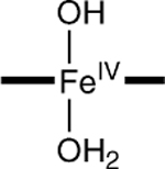
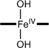
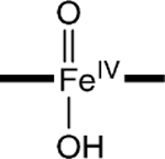
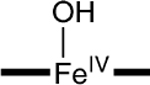
Influence of Axial Ligands in [Fe^IV(X)(Y)B*]ⁿ⁻ (X/Y = O, −OH, and H₂O) on Isomer Shift δ, Quadrupole Splitting ΔE_Q, and Fe—O Distance^a

FeIV Model Complex	δ (mm/s)	ΔEQ (mm/s)	Fe—O (Å)
	−0.11	5.1	1.80,‡ 2.27‡
	−0.15	3.6	1.88‡, 1.88‡
	−0.07‡	1.6‡	1.69, 2.05‡
	−0.07‡	4.4	1.80‡
	−0.12	3.5	1.65
b	−0.14	4.0	1.68
Experiment	−0.19(2)c	3.95(3)c	1.69(2) d

^aProperties obtained by DFT calculations for the geometry-optimized structure in the S = 1 state.

^bTwo water molecules are hydrogen-bonded to axial oxygen; see Figure S1 in the Supporting Information for the optimized structure.

^cFrom Mossbauer analysis.

^dFrom EXAFS analysis.

^‡Violates one of the three conditions given in the text.

Figure 10.

Correlation between DFT calculated and experimental quadrupole splittings for three different ligand systems.^4,6,19,20 The factor for the conversion of the quadrupole splitting from atomic units to mm/s is taken as −1.43 mm s⁻¹/AU to obtain a regression line with a slope of 1. Correlation coefficient R² is 0.96. Complex 2 is indicated with a solid dot.

Figure 9.

Correlation between DFT calculated and experimental isomer shifts for three different ligand systems.^4,6,19,20 TAML complexes are listed to the right of the regression line. The correlation coefficient R² is 0.99. Complex 2 is indicated with a solid dot.

3. Results and Discussion

3.1. Electronic Absorption and Mössbauer Studies.

The addition of tert-butyl hydroperoxide (TBHP) to an aqueous solution of Na[Fe^III(H₂O)B*] (1), prepared in 0.1 M KOH solution (or 0.1 M phosphate buffer of pH 13.7), generates a red species (2, λ_max = 435 nm; Figure 2). Species 2 is quite stable at room temperature, decaying by less than 10% in 2 h. A titration of 1 with TBHP revealed that ca. 0.5 equiv of oxidant per Fe^III is required to obtain the maximum yield of 2 (inset in Figure 2), indicating the formation of a Fe^IV species. A one-to-one transformation of 1 to 2 is indicated by an isosbestic point at 350 nm. Quantitation of 2 by Mössbauer spectroscopy (see below) yielded the extinction coefficient ε₄₃₅ = 2500(200) M⁻¹ cm⁻¹.

Figure 2.

Formation of 2 (bold solid line) from 1 (dashed line) by addition of 0.5 equiv of TBHP, at pH 14, over a time period of ~10 min. Inset shows the changes in absorption at 435 nm as a function of the number of TBHP equivalents added.

We have studied samples of 2 with Mössbauer spectroscopy between 4.2 and 140 K in applied magnetic fields up to 8.0 T. Three representative spectra are shown in Figure 3. In zero field, complex 2 exhibits a doublet with quadrupole splitting, ΔE_Q = 3.95(3) mm/s, and isomer shift, δ = −0.19(2) mm/s. As shown below in the discussion of Figures 9 and 10, these parameters are characteristic of S = 1 Fe^IV–TAML complexes. We have analyzed the applied field spectra with the S = 1 spin Hamiltonian

$$\begin{array}{l}H=D\left({\widehat{S}}_z^2-2/3\right)+E\left({\widehat{S}}_x^2-{\widehat{S}}_y^2\right)+\beta \widehat{\mathbf{S}}\cdot \mathbf{g}\cdot \mathbf{B}+\widehat{\mathbf{S}}\cdot \mathbf{A}\cdot \widehat{\mathbf{I}}-\\ g_{\text{n}}{\beta }_{\text{n}}\mathbf{B}\cdot \widehat{\mathbf{I}}+\left(eQ{V}_{zz}/12\right)\left[3{\widehat{I}}_z^2-15/4+\eta \left({\widehat{I}}_x^2-{\widehat{I}}_y^2\right)\right]\end{array}$$ (1)

where D and E are zero-field splitting (ZFS) parameters, B is the applied magnetic field, I is the nuclear spin of ⁵⁷Fe, and A is the magnetic hyperfine tensor. The solid lines in Figure 3 are spectral simulations (to a set of eight spectra) based on eq 1, using the parameters listed in Table 1. Similar to most S = 1 Fe^IV complexes,^19,20,36 2 exhibits a large and positive zero-field splitting, D = 24(3) cm⁻¹. Neese and coworkers^13,14 and others^19,20 have ascribed the large D values to contributions arising from spin–orbit coupling of the S = 1 ground state with excited S = 2 and S = 0 states. In section 3.4.4, the contributions to D from S = 0, 1, and 2 are estimated for complex 2. If the coupling of the ground state with S = 1 states from the t_2g manifold provides a significant contribution to D, there is an attendant reduction in the magnitude of the x and y components of the A tensor and an increase in g_x and g_y.³⁷ In contrast, the spin–orbit coupling of the S = 1 ground state with S = 2 and S = 0 excited states, while contributing to D, has no first-order effect on g and A.³⁸ The x and y components of A listed in Table 1 are among the largest in magnitude observed for S = 1 Fe^IV complexes; below, we will rationalize this observation. The Mössbauer parameters of 2 establish this complex as a S = 1 Fe^IV species.

Figure 3.

Mössbauer spectra (4.2 K) of 2 in aqueous solution, at pH 14, recorded in parallel-applied fields 0 T (A), 2.0 T (B), and 8.0 T (C). The solid lines are spectral simulations based on eq 1 using the parameters listed in Table 1. At least 95% of the iron in the sample belongs to 2.

3.2. XAS Studies.

Information about the structural nature of 2 is obtained from X-ray absorption spectroscopic studies at the Fe K edge (Figure 4). A sample in frozen aqueous solvent, more than 90% pure in 2 according to Mössbauer spectroscopy, exhibits a K edge at 7124.5 eV, which is 0.6 eV higher than the K edge for [Fe^III(H₂O)B*]⁻ and 0.8 eV lower than the edge for [Fe^V(O)B*]⁻.⁶Similarly, the pre-edge peak of 2 at 7113.5 eV is found to be 0.5 eV higher than that of [Fe^III(H₂O)B*]⁻ and 0.6 eV lower than that of [Fe^V(O)B*]⁻.⁶ These observations support the Mössbauer assignment that 2 is a Fe^IV complex. The 1s → 3d pre-edge transition found for 2 is rather intense, with an area of 41 units (Figure 4A), which is halfway in between the values of 17 units for [Fe^III(H₂O)B*]⁻ and 60 units for [Fe^V(O)B*]⁻. The pre-edge peak area of 2 is larger than any observed to date for S = 1 oxo–iron(IV) species, the areas of which range from 18 to 38 units.^20,39

Figure 4.

(A) Fe K-edge X-ray absorption near-edge structure (XANES, fluorescence excitation) of [Fe^IV(O)B*]²⁻ (2). (B) Fourier transform of the Fe K-edge EXAFS data (k³χ(k)) and Fourier-filtered EXAFS spectra (k³χ′(k), inset) for [Fe^IV(O)B*]²⁻ (2). Fourier transform range k = 2–15 Å⁻¹; back-transform range r′ = 0.40–3.10 Å; fit with parameters listed in fit 6 in Table 2. Dots, experimental data; solid lines, fits.

Direct evidence that 2 is a Fe^IV═O complex was obtained from the analysis of the EXAFS region of the X-ray absorption spectrum (Figure 4B). The best fit obtained consisted of three shells, namely, one O scatterer at 1.69 Å, four N/O scatterers at 1.90 Å, and five C scatterers at 2.84 Å (Table 2). The scatterers at 1.90 and 2.84 Å are consistent with low Z atoms of the macrocyclic ligand as found in the EXAFS fits for [Fe^III(H₂O)B*]⁻ and [Fe^V(O)B*]⁻ complexes; the coordination number of the C shell is lower than the expected value of 8 because of the distribution of Fe· · ·C distances, which differ by as much as 0.12 Å in the crystal structure of the (μ-oxo)diiron(IV)–TAML complex.⁵ Most importantly, the 1.69 Å scatterer can be assigned to the oxo atom of a Fe–O unit, with a distance that is 0.10 Å longer than obtained for the [Fe^V(O)B*]⁻ complex⁶ but 0.04 Å shorter than the Fe–O distance obtained in the crystal structure of the (μ-oxo)diiron(IV)–TAML complex.⁵

3.3. pH Dependence.

To assess the pH range of the stability of complex 2, we have conducted electronic absorption spectroscopy and Mössbauer studies between pH 14 and 8.6. When the pH of a preformed solution of 2 was changed from pH 13 to 8.6 (10 mM phosphate buffer), significant changes in the electronic absorption spectrum occurred instantly (<1 s). The new species (Figure 5) exhibits a spectral pattern similar to that for the μ-oxo-bridged [B*Fe^IV–O–Fe^IVB*]²⁻ species, 3, reported by Ghosh et al.⁵ Figure 6A shows a 4.2 K Mössbauer spectrum recorded after freezing a TBHP-oxidized sample prepared at pH 8.6. The spectrum exhibits a doublet (ca. 75% of Fe) with ΔE_Q = 3.25(3) mm/s and δ = −0.07(2) mm/s. These parameters are essentially identical to those reported for the diamagnetic Fe^IV–O–Fe^IV complex, 3 (ΔE_Q = 3.3 mm/s, δ = −0.07 mm/s, observed in the solid and in acetonitrile). Studies in strong applied magnetic fields (not shown) demonstrate that the ΔE_Q = 3.25 mm/s species observed here is indeed diamagnetic, in support of assigning this doublet to 3. The pH 8.6 sample exhibits a second doublet with ΔE_Q = 4.7 (1) mm/s and δ = −0.20(4) mm/s that represents ca. 12% of the Fe in the sample (spectrum drawn to scale above the data of Figure 6A). This species, on the basis of the isomer shift and the observation of a doublet in zero applied field, is an Fe^IV complex of unidentified nature. The sample also contains a minor paramagnetic component with unresolved features. EPR studies (not shown) suggest that this component belongs to a Fe^IIIFe^IV dimer (This complex presently is being studied in the laboratories of T. J. Collins and M. P. Hendrich at Carnegie Mellon University).

Figure 6.

Zero-field 4.2 K Mössbauer spectra of 1 oxidized with TBHP at pH 8.6 (A) and pH 11.7 (B). The major doublet in A, accounting for ~76% of Fe, belongs to [B*Fe^IV–O–Fe^IVB*]²⁻, 3. A second doublet (drawn separately above the data, ~12%) with ΔE_Q = 4.7(1) mm/s and δ = −0.20 (4) mm/s belongs to an as yet unidentified Fe^IV species. (B) Sample was prepared at pH 11.7 and then frozen by immersion into liquid nitrogen. The solid line is a superposition of two doublets belonging to mononuclear complex 2 (46%) and dimer 3 (43%).

Figure 7 shows a plot of the absorbance at 765 and 1050 nm (bands assigned to 3) as a function of pH. This titration indicates a pK_a near 10. However, a Mössbauer sample prepared at pH 11.7 exhibits two doublets (Figure 6B), belonging to 2 (46%) and 3 (43%). A study of the pH dependence with Mössbauer spectroscopy (in frozen solution) showed the transition between 2 and 3 to be compressed into a narrow pH range of 11.6–11.9. We suspect that pH changes of the phosphate buffer upon freezing^40,41 are responsible for the different behavior observed between room-temperature electronic absorption and frozen solution Mössbauer studies.

We thus have in hand two iron(IV)–oxo complexes of B* that can be inter-related by a pH equilibrium. Starting from 3, complex 2 can be formed by increasing the pH to above 12. This transformation can be reversed by lowering the pH. [Fe^IV(O)B*]²⁻ in turn is in principle related to [Fe^V(O)B*]⁻ by one-electron transfer. However, the different solvent conditions under which these two complexes are generated hamper efforts to establish this relationship. For example, the highly basic aqueous conditions needed to generate and stabilize [Fe^IV(O)B*]²⁻ give rise to background signals in the cyclic voltammetric scans that potentially obscure the anticipated Fe^V/IV wave. As an alternative strategy, we attempted chemical reductions of [Fe^V(O)B*]⁻ and found that this complex can be reduced by dicacetylferrocene (E_1/2 = 490 mV versus Fc) in acetonitrile to afford the (μ-oxo)diiron(IV) complex, 3. Presumably, electron transfer to [Fe^V(O)B*]⁻ initially forms [Fe^IV(O)B*]²⁻, which because of its high basicity readily acquires a proton from the solution and converts to the dimer.⁵ This result allows us to estimate the Fe^V/IV potential to be greater than 490 mV versus Fc. This value is not unreasonable, considering the reported electrochemistry of [B*Fe^IV–O–Fe^IVB*]²⁻ that shows a one-electron reduction at −230 mV versus Fc (Fe^IVFe^IV/Fe^IIIFe^IV) and two one-electron oxidations at +370 and +720 mV (formally Fe^VFe^IV/Fe^IVFe^IV and Fe^VFe^V/Fe^IVFe^V, respectively).⁵

The properties of [B*Fe^IV–O–Fe^IVB*]²⁻ (3), [Fe^IV(O)B*]²⁻ (2), and [Fe^V(O)B*]⁻ characterized to date should allow us to assess the roles of these high-valent Fe–B* species in the complex reactivity profile for the numerous demonstrated catalytic transformations with tightly pH-determined interrelationships.

3.4. DFT Calculations.

3.4.1. Axial Coordination.

To assess the axial coordination of 2, we have conducted DFT calculations for a series of plausible axial ligands. These formulations of the complex have been listed in Table 3, together with the DFT values for the ⁵⁷Fe isomer shifts, quadrupole splittings, and Fe–O distances predicted for the species. The obvious candidate, [Fe^IV(O)(H₂O)B*]²⁻, has not been listed because the axial water molecule dissociates in the course of the geometry optimization.

The parameter values calculated for the species of Table 3 can be compared to the experimental data for complex 2 listed at the bottom of the table. Our DFT experience with TAML complexes suggests that, for an acceptable description of 2, the parameters should roughly satisfy the following conditions: |δ − δ_exp| < 0.08 mm/s, |ΔE_Q − ΔE_Q,exp| < 1.0 mm/s, and bond-length difference |(Fe–O) – (Fe–O)_exp| < 0.05 Å. Entries in the table that violate one of the conditions are marked (‡). The table shows that complexes with axial ligands other than O have at least one parameter outside the specified range. We conclude from this result that spectroscopic species 2 is the intermediate-spin (S = 1) five-coordinate complex [Fe^IV(O)B*]²⁻. A picture of the geometry-optimized structure of the complex is shown in Figure 8.

The gas-phase value for [Fe^IV(O)B*]²⁻, δ = −0.12 mm/s, is 0.07 mm/s larger than the experimental target. The agreement is not quite satisfactory but is slightly improved when the axial oxygen is hydrogen-bonded to two water molecules (seventh row of Table 3), obtaining δ = −0.14 mm/s. The hydrogen bonding further improves the agreement of the calculated values for ΔE_Q and the Fe–O distance with the experimental data. The Fe–O bond length increases by 0.03 Å under the influence of the two water molecules and is within the error margin equal to the value deduced from the EXAFS data [1.69(2) Å]. The calculated isomer shift of the new species is halfway between the values found for Fe^III– and Fe^V–TAML complexes and supports the identification of 2 as a Fe^IV species. The value calculated for the quadrupole splitting of 2 gives a large, positive value, which distinguishes it from the ΔE_Q = 0.89 mm/s (D = −2.6 cm⁻¹) of the only known S = 2 Fe^IV–TAML complex, [Fe^IV(Cl)MAC*]⁻. In the following sections, we discuss the electronic structure of 2, on the basis of a comparison of the spectroscopic observables for 2 with those for other Fe^IV species.

3.4.2. Isomer Shift.

In the past 3 years, we have studied a variety of Fe^IV complexes, experimentally as well as theoretically.^4–6,19,20 Nonheme Fe^IV═O complexes are now available for three equatorial ligand combinations with widely differing donor strengths; weak, medium, and strong nonoxo donors are found in [Fe^IV(O)(H₂O)₅]²⁺,¹⁹ [Fe^IV(O)(MeCN)TMC]⁺,²⁰ and [Fe^IV(O)B*]²⁻, respectively. The increasing ligand field in the series causes a steep rise in the energy of the x²−y² orbital and transforms the orbital configuration (spin) (xy)¹(xz)¹(yz)¹(x²−y²)¹ (S = 2) for the aqueous species into (xy)²(xz)¹(yz)¹ (S = 1) for the two complexes with macrocyclic nitrogen donors.

The donor properties of the equatorial ligands have a strong influence on the Mössbauer parameters of these systems. Figure 9 shows experimental and calculated isomer shifts (see the Materials and Methods) for a collection of Fe^III, Fe^IV, and Fe^V compounds.^4,6,16,19,20 The overall correlation between the experiment and theory is excellent. The isomer shift is a reliable indicator of the iron oxidation state in the comparison of complexes with similar equatorial ligands: δ(Fe^III) > δ(Fe^IV) > δ(Fe^V). This trend is observed for all three ligand systems. For example, in the case of the TAML complexes, δ([Fe^III(Cl)MAC*]²⁻) = +0.25 mm/s > δ([Fe^IV(Cl)MAC*]⁻) = −0.05 mm/s and δ([Fe^IV(O)B*]²⁻) = −0.19 mm/s > δ([Fe^V(O)B*]⁻) = −0.39 mm/s. The removal of a 3d electron reduces the shielding of the iron nucleus and leads to a contraction of the occupied s orbitals, increasing the s electron density at the nucleus, and therefore, gives a lowering of the isomer shift.⁴²

The isomer shifts of the Fe^IV═O species are dispersed over a remarkably broad range, from +0.39 to −0.19 mm/s, owing to the wide disparity in the donor capacities of the equatorial ligands. The effect of electron donation on δ depends upon the type of the acceptor orbital: thus, donation to a 3d orbital increases δ, whereas donation to 4s decreases the shift.⁴² Because the 4s effect dominates,^29,35,43,44 there is a decrease in the isomer shift as a function of the increasing equatorial donor strength, e.g., δ([Fe^IV(O)(H₂O)₅]²⁺) = +0.39 mm/s > δ([Fe^IV(O)(NCMe)(TMC)]²⁺) = +0.16 mm/s > δ([Fe^IV(O)B*]²⁻) = −0.19 mm/s. As a consequence, the Fe^III–TAML complexes in Figure 9 have δ values similar to those of the Fe^IV complexes with TMC and TMCS ligands, despite the difference in their formal oxidation states. The high-spin (S = 2) iron sites in [Fe^IV(O)(H₂O)₅]²⁺ and [Fe^IV(Cl)MAC*]⁻ have substantially different isomer shifts (+0.39 versus −0.05 mm/s), showing that there is no unique relationship between the isomer shift and spin of Fe^IV sites.

The oxidation of [Fe^III(H₂O)DMOB]⁻, where DMOB is the dimethoxy analogue of B*, is ligand-based and has virtually no effect on the isomer shift (see Figure 9). Conditions for ligand versus metal-based oxidation of TAML complexes have been discussed in ref 4.

3.4.3. Quadrupole Splitting ΔE_Q.

Figure 10 displays the correlation between experimental and calculated quadrupole splittings, ΔE_Q.^4,6,16,19,20 Although the agreement is less satisfactory than in the case of the isomer shift, the calculations reproduce the marked trend in the dependence of ΔE_Q on ligand type. The systems in the right, upper corner of the figure are all TAML complexes. The large positive ΔE_Q values for these systems are due to the oblate (disk-shaped) charge distribution around the iron nucleus, arising from the large electronic charge donated by the N¹⁻ amido groups into the x²−y² orbital. The ΔE_Q values for the Fe^III–, Fe^IV–, and Fe^V–TAML complexes are remarkably similar. All Fe^III species have the S = 3/2 configuration (xy)²(xz)¹(yz)¹(z²)¹, yielding a vanishing valence contribution to the quadrupole splitting, ~0 mm/s, whereas the valence term of the S = 1 configuration (xy)²(xz)¹(yz)¹ of the Fe^IV complexes contributes ~ +4 mm/s. However, the large increase in the valence contribution to ΔE_Q caused by the removal of the z² electron is largely compensated by donation of electron density from the axial ligand into the vacated spin–orbital (z²)^α and because the axial bonds of Fe^IV are stronger than those of Fe^III, by increased electron donations from the axial ligand(s) into (xz)^β, (yz)^β, and (z²)^β, which are vacant in both the Fe^III and Fe^IV species (in this discussion, α is the spin of the electrons carrying the majority spin of the iron). The axial donations add up to a prolate (or spheroid generated by rotating an ellipse around its longer axis) charge distribution around the iron nucleus, contributing a negative term to ΔE_Q that nearly compensates the effect of the loss of the z² electron. In passing, we note that ΔE_Q, similar to δ, is hardly affected by the oxidation of the benzene moiety of the [Fe^III(H₂O)DMOB]⁻ complex (Figure 10).

With the exception of [Fe^IV(Cl)MAC*]⁻, the TAML complexes in Figure 10 have larger ΔE_Q values than the non-TAML species, because TAMLs are substantially stronger σ donors. The MAC* complex differs from the other Fe^IV–TAML complexes in that the iron has the high spin (S = 2) configuration (xy)¹(xz)¹(yz)¹(z²)¹.⁴⁵ The valence contribution (~ −4 mm/s) of the MAC* species cancels almost completely against the large equatorial ligand contribution (~ +3 mm/s), yielding a small net quadrupole splitting of ~ −0.9 mm/s. [Fe^IV(O)(H₂O)₅]²⁺ is also high spin, but with orbital configuration (xy)¹(xz)¹(yz)¹(x²−y²)¹. Here, the valence contribution (~ +4 mm/s) is compensated by the large, negative axial contribution to ΔE_Q of the oxo ligand, resulting in a small value for ΔE_Q.

3.4.4. Zero-Field Splitting, g Values, and Magnetic Hyperfine Coupling.

On the basis of SCF calculations for the S = 0, 1, and 2 states of [Fe^IV(O)B*]²⁻ and the application of TD DFT to the S = 1 ground state, we have estimated energies for both the spin-forbidden and spin-allowed d–d transitions of complex 2 (cf. Supporting Information). Through spin–orbit coupling, the excited states have a profound influence on the spectroscopic properties of the S = 1 ground multiplet.^13,14 In the Supporting Information, we present expressions for the zero-field splitting (D),²⁰ the deviation of the g values from the free-electron value (Δg), and a nonvanishing orbital term in the magnetic hyperfine coupling (A^L). The expressions for D are similar but not identical^20,46 to those given in refs 13 and 14. The analysis adopted here takes into account covalency,³⁸ which causes a significant reduction in the value for D and related observables. The estimated value D = 26.5 cm⁻¹ (see the Supporting Information) is in good agreement with the experimental data, D = 24(3) cm⁻¹, and contains contributions for the three possible values of the spin of a d⁴ system: D = D_S=0 + D_S=1 + D_S=2. The spin states contribute D_S=0 = +10.5 cm⁻¹, D_S=1 = +10.8 cm⁻¹, and D_S=2 = +5.2 cm⁻¹, indicating that the contribution from excited S ≠ 1 states is larger than those from S = 1 states. Taking the S = 1 ground configuration {xy^αxy^βxz^αyz^α} as a reference, D_S=0 can be assigned to the spin-forbidden transitions xz^α → yz^β and y^α → xz^β, D_S=1 to a predominant (~7 cm⁻¹) contribution from the spin-conserving transitions xz^α → (z²)^α and yz^α → (z²)^α, and D_S=2 to the spin-forbidden transition xy^β → (x²−y²)^α.

In 1974, Oosterhuis and Lang³⁷ gave the crystal-field expressions for the zero-field splitting and the g and A tensors for the S = 1 ground multiplet of a (t_2g)⁴ configuration. The Oosterhuis and Lang (O–L) model considers spin–orbit coupling between the three S = 1 states generated when the β electron is placed into xy, yz, or xz. The O–L model is based on the assumption that the following interactions can be ignored: (i) spin–orbit coupling of the S = 1 ground state with S ≠ 1 excited states and (ii) spin–orbit coupling of the ground state with S = 1 excitations to the e_g levels. Given the large “outer-spin-state” contributions to D (see above),³⁸ it is clear that condition (i) is violated in 2. However, because the selection rule ΔS = 0 for spin-independent interactions implies that spin–orbit coupling between multiplets of different spin has no first-order effect on the g values and the orbital contribution to the magnetic hyperfine tensor, the O–L model may still provide a good description for these quantities, unless condition (ii) is violated as well. The O–L expressions show that g_x and g_y increase as the t_2g crystal-field splittings decrease, so that Δg_⊥ = g_⊥ − 2 > 0. As we shall show below, this is not the case in 2.

The magnetic hyperfine tensor is, in general, the sum of the Fermi-contact, spin-dipolar, and orbital terms: A = A^FC + A^SD + A^L. When spin–orbit coupling is treated in the second-order perturbation theory, the orbital contribution to the magnetic hyperfine tensor, A^L_⊥, is proportional to PΔg_⊥ (see Chapter 19 in ref 47), where P = 2βg_nβ_n〈r⁻³〉. Thus, for Δg_⊥ > 0, the orbital term opposes the (negative) Fermi-contact contribution and leads to a reduction in A_⊥. In our previous work on Fe^IV–TMC complexes,²⁰ we observed large D values (D ≈ 20–35 cm⁻¹) as in the TAML complex, but without an apparent reduction in A_⊥. These observations indicated that the main contributions to D resulted from spin–orbit mixing of the S = 1 ground state with S = 2 and 0 excited states (see above).^13,14,20

Our DFT calculations of [Fe^IV(O)B*]²⁻ suggest the presence of S = 1 excited states at ~10 000 cm⁻¹, which result from xz, yz → z² excitations (Table S1 in the Supporting Information). Mixing of these states with the S = 1 ground state produces a Δg_⊥ < 0 and thus a negative contribution to A_⊥. Our calculations, described in sections S1–S3 in the Supporting Information, suggest that Δg_⊥ = −0.04 and g_⊥ = 1.96 for [Fe^IV(O)B*]²⁻. Thus, condition (ii) of the O–L model is not fulfilled either in 2 [As worked out in the seminal paper of Neese and Solomon,³⁸ the signs of the contributions to Δg_⊥ and A^L_⊥ (eq S7 in the Supporting Information) depend upon the occupation numbers of the initial and final orbital states of the excited electron: a (half-filled → empty transition) gives a negative term and a (filled → half-filled) transition yields a positive term (cf. eq S7 in the Supporting Information)]. This effect might explain why the experimental A_x and A_y values are ca. 2–3 T larger in magnitude than those observed previously for Fe^IV═O complexes.³

The principal axes of A^SD and A^L in [Fe^IV(O)B*]²⁻ coincide with the x, y, and z axes (Figure 8) used in the discussion of the 3d orbitals (NB the principal axes in the x−y plane are defined apart from a rotation because of eigenvalue degeneracy). For the optimized geometry of Figure 8, our DFT calculations for the spin-dipolar term yield the components A^SD = (−7, −7, and +14) T. A calculation for the |xy^αxy^βxz^αyz^α| ground state gives A^SD = (−1/7, −1/7, and +2/7)P, yielding P = 49 T, in excellent agreement with the empirical value P = 50 T that we have used for Fe^IV–TMC complexes in earlier work.²⁰ Using the DFT values obtained for P together with Δg_⊥ = −0.04 and Δg_z = 0 yields for the orbital term A^L = (−2, −2, and 0) T. The isotropic part of the A tensor A^iso = (A_x + A_y + A_z)/3 comprises the Fermi-contact contribution and a small orbital (pseudo-contact) contribution A^L,iso = PΔg_av = −1.3 T, where Δg_av = g_av − 2 and g_av = (g_x + g_y + g_z)/3. For complex 2, we have A^iso(exp) = −17.3 T, yielding A^FC(exp) = −16 T. The contact term is generally poorly described by DFT (a correction factor of 1.8 has been suggested in ref 18). The contact term is often expressed as A^FC = κP, yielding κ ≈ 0.33. Summing the three contributions yields A = A^FC + A^SD + A^L ≈ (−25, −25, and −2) T, which describes well the two large negative components along x and y and the nearly vanishing component along z. The contact term is a measure of the spin delocalization of the metal site. In this context, it is interesting to note that [Fe^V(O)B*]⁻ has A^FC = −18 T, indicating some degree of spin polarization of the electron density donated by oxygen into the vacated xzorbital.

3.4.5. Comparison of 2 with Other Nonheme Iron(IV)–Oxo Complexes.

The S = 2 ground configuration of [Fe^IV(O)(H₂O)₅]²⁺ (see section 3.4.3) and the S = 1 ground configurations of [Fe^IV(O)B*]²⁻ and [Fe^IV(O)(NCMe)(TMC)]²⁺ are interchangeable by the spin-forbidden transitions xy^β ↔ (x²−y²)^α. The spin–orbit coupling between these two states has been proposed as the principal mechanism for generating the zero-field splittings in both [Fe^IV(O)(H₂O)₅]²⁺ (D = 9 cm⁻¹) and [Fe^IV(O)(NCMe)(TMC)]²⁺ (D = 29 cm⁻¹) (see refs 13, 16, 19, and 20). However, this mechanism furnishes only a secondary contribution to D in [Fe^IV(O)B*]²⁻ (see section 3.4.4). The difference between the two S = 1 species can be explained as follows. As shown in Table 4, the Fe–N distances in the TAML species are shorter than in the TMC species. As a consequence, the energy of the spin-forbidden xy → x²−y² transition to the S = 2 excited state in the TAML species is higher than in the TMC species, leading to a smaller value for D_S=2 for the TAML species (see section 3.4.4). However, the smaller value for D_S=2 is partially off-set by a larger value for D_S=1 in the TAML species: because the Fe–O distance in the TAML species is longer than in the TMC species (Table 4), the xz, yz → z² energy is lower, and the associated value for D_S=1 (see section section 3.4.4) is therefore higher than for the TMC complex, leading altogether to a slightly smaller value for D (Table 4). The values for the hyperfine parameters in Table 4 corroborate the larger ligand strength of TAMLs relative to TMC: the B* complex has a smaller δ value than the TMC complex because of increased charge donation into the 4s orbital (see section 3.4.2), a larger ΔE_Q value resulting from an increased in-plane and reduced axial electron donation (see section 3.4.3), and a smaller A_⊥ value (see section 3.4.4) originating from the increase in the orbital angular momentum in the x, y plane attending the increase in D_S=1 (see above).

Table 4.

Comparison of Parameters for [Fe^IV(O)B*]²⁻ and [Fe^IV(O)(NCMe)TMC]²⁺⁴⁸

	TAML	TMC
Fe—Neqa	1.90b	2.09b
Fe—O (Å)	1.69	1.65
δ (mm/s)	−0.19	+0.17
ΔEQ (mm/s)	+3.95	+1.23
A⊥ (T)	−27.0	−22.5
D (cm−1)	+24	+29

^aeq = equatorial.

^bAverages.

The Fermi-contact terms for [Fe^IV(O)(H₂O)₅]²⁺ (A^FC = −25 T, ref 19), [Fe^IV(O)(NCMe)(TMC)]²⁺ (A^FC = −15 T, refs 16 and 20), and [Fe^IV(O)B*]²⁻ (A^FC = −16 T) imply contributions to the internal field of −12.5, −7.5, and −8 T/unpaired electron, respectively. These values indicate that the delocalization of the iron spin onto the ligands in the TMC and TAML species is significantly larger than in the aqueous complex.

In conclusion, the differences in the fine- and hyperfine-structure parameters for the TAML and TMC species in Table 4 are a consequence of the strong donor properties of the TAML and support the identification of 2 as a [Fe^IV(O)TAML]²⁻ complex.

References

- (1).Collins TJ Acc. Chem. Res. 2002, 35, 782–790. [DOI] [PubMed] [Google Scholar]
- (2).Collins TJ; Walter C Sci. Am. 2006, 294, 83–90. [DOI] [PubMed] [Google Scholar]
- (3).Costas M; Mehn MP; Jensen MP; Que L Jr. Chem. Rev. 2004, 104, 939–986. [DOI] [PubMed] [Google Scholar]
- (4).Chanda A; Popescu D-L; Tiago de Oliveira F; Bominaar EL; Ryabov AD; Münck E; Collins TJ J. Inorg. Biochem. 2006, 100, 606–619. [DOI] [PubMed] [Google Scholar]
- (5).Ghosh A; Tiago de Oliveira F; Yano T; Nishioka T; Beach ES; Kinoshita I; Münck E; Ryabov AD; Horwitz CP; Collins TJ J. Am. Chem. Soc. 2005, 127, 2505–2513. [DOI] [PubMed] [Google Scholar]
- (6).Tiago de Oliveira F; Chanda A; Banerjee D; Shan X; Mondal S; Que L Jr.; Bominaar EL; Münck E; Collins TJ Science 2007, 315, 835–838. [DOI] [PubMed] [Google Scholar]
- (7).Groves JT J. Inorg. Biochem. 2006, 100, 434–447. [DOI] [PubMed] [Google Scholar]
- (8).Hanson LK; Chang CK; Davis MS; Fajer J J. Am. Chem. Soc. 1981, 103, 663–670. [Google Scholar]
- (9).Roberts JE; Hoffman BM; Rutter R; Hager LP J. Am. Chem. Soc. 1981, 103, 7654–7656. [Google Scholar]
- (10).Decker A; Clay MD; Solomon EI J. Inorg. Biochem. 2006, 100, 697–706. [DOI] [PubMed] [Google Scholar]
- (11).Decker A; Rohde J-U; Que L Jr.; Solomon EI J. Am. Chem. Soc. 2004, 126, 5378–5379. [DOI] [PubMed] [Google Scholar]
- (12).Decker A; Solomon EI Angew. Chem., Int. Ed. 2005, 44, 2252–2255. [DOI] [PubMed] [Google Scholar]
- (13).Schöneboom JC; Neese F; Thiel W J. Am. Chem. Soc. 2005, 127, 5840–5853. [DOI] [PubMed] [Google Scholar]
- (14).Neese F J. Inorg. Biochem. 2006, 100, 716–726. [DOI] [PubMed] [Google Scholar]
- (15).Conradie MM; Conradie J; Ghosh A J. Inorg. Biochem. 2006, 100, 620–626. [DOI] [PubMed] [Google Scholar]
- (16).Rohde J-U; In J-H; Lim MH; Brennessel WW; Bukowski MR; Stubna A; Münck E; Nam W; Que L Jr. Science 2003, 299, 1037–1039. [DOI] [PubMed] [Google Scholar]
- (17).Balland V; Charlot MF; Banse F; Girerd JJ; Bill E; Bartoli JF; Battioni P; Mansuy D Eur. J. Inorg. Chem. 2004, 301–308. [Google Scholar]
- (18).Sinnecker S; Slep LD; Bill E; Neese F Inorg. Chem. 2005, 44, 2245–2254. [DOI] [PubMed] [Google Scholar]
- (19).Pestovsky O; Stoian S; Bominaar EL; Shan X; Münck E; Que L Jr.; Bakac A Angew. Chem., Int. Ed. 2005, 44, 6871–6874. [DOI] [PubMed] [Google Scholar]
- (20).Bukowski MR; Koehntop KD; Stubna A; Bominaar EL; Halfen JA; Münck E; Nam W; Que L Jr. Science 2005, 310, 1000–1002. [DOI] [PubMed] [Google Scholar]
- (21).Horwitz CP; Ghosh A Synthesis patent: US 7060818 B2, 2006.
- (22).George GN EXAFSPAK, Stanford Synchrotron Radiation Laboratory, Stanford Linear Accelerator Center, 1990. [Google Scholar]
- (23).Scarrow RC; Maroney MJ; Palmer SM; Roe AL; Que L Jr.; Salowe SP; Stubbe J J. Am. Chem. Soc. 1987, 109, 7857–7864. [Google Scholar]
- (24).Scarrow RC; Trimitsis MG; Buck CP; Grove GN; Cowling RA; Nelson MJ Biochemistry 1994, 33, 15023–15035. [DOI] [PubMed] [Google Scholar]
- (25).Becke AD J. Chem. Phys. 1993, 98, 5648. [Google Scholar]
- (26).Lee C; Yang W; Parr RG Phys. ReV. B: Condens. Matter Mater. Phys. 1988, 37, 785. [DOI] [PubMed] [Google Scholar]
- (27).Frisch MJ; Trucks GW; Schlegel HB; Scuseria GE; Robb MA; Cheeseman JR; Montgomery JAJ; Vreven T; Kudin KN; Burant JC; Millam JM; Iyengar SS; Tomasi J; Barone V; Mennucci B; Cossi M; Scalmani G; Rega N; Petersson GA; Nakatsuji H; Hada M; Ehara M; Toyota K; Fukuda R; Hasegawa J; Ishida M; Nakajima T; Honda Y; Kitao O; Nakai H; Klene M; Li X; Knox JE; Hratchian HP; Cross JB; Bakken V; Adamo C; Jaramillo J; Gomperts R; Stratmann RE; Yazyev O; Austin AJ; Cammi R; Pomelli C; Ochterski JW; Ayala PY; Morokuma K; Voth GA; Salvador P; Dannenberg JJ; Zakrzewski VG; Dapprich S; Daniels AD; Strain MC; Farkas O; Malick DK; Rabuck AD; Raghavachari K; Foresman JB; Ortiz JV; Cui Q; Baboul AG; Clifford S; Cioslowski J; Stefanov BB; Liu G; Liashenko A; Piskorz P; Komaromi I; Martin RL; Fox DJ; Keith T; Al-Laham MA; Peng CY; Nanayakkara A; Challacombe M; Gill PMW; Johnson B; Chen W; Wong MW; Gonzalez C; Pople JA Gaussian, Inc., Wallingford CT, 2004. [Google Scholar]
- (28).In earlier reports, we used the factor −1.6 mm s−1/AU. The set of high-oxidation complexes considered here require a slightly smaller factor. As for the isomer shift, the calibration constant for the quadrupole splitting depends upon the basis set and functional and is considered here as a semi-empirical parameter.
- (29).Vrajmasu V; Münck E; Bominaar EL Inorg. Chem. 2003, 42, 5974–5988. [DOI] [PubMed] [Google Scholar]
- (30).Nieuwpoort WC; Post D; Duijnen PT Phys. ReV. B: Condens. Matter Mater. Phys. 1978, 17, 91–98. [Google Scholar]
- (31).Reschke R; Trautwein AX; Desclaux JP J. Phys. Chem. Solids 1977, 38, 837–841. [Google Scholar]
- (32).Han WG; Liu T; Lovell T; Noodleman L J. Comput. Chem. 2006, 27, 1292–1306. [DOI] [PubMed] [Google Scholar]
- (33).Liu T; Lovell T; Han WG; Noodleman L Inorg. Chem. 2003, 42, 5244–5251. [DOI] [PubMed] [Google Scholar]
- (34).Zhang Y; Mao J; Oldfield E J. Am. Chem. Soc. 2002, 124, 7829–7839. [DOI] [PubMed] [Google Scholar]
- (35).Neese F Inorg. Chim. Acta 2002, 337C, 181–192. [Google Scholar]
- (36).Lim MH; Rohde J-U; Stubna A; Bukowski MR; Costas M; Ho RYN; Münck E; Nam W; Que L Jr. Proc. Nat. Acad. Sci. U.S.A. 2003, 100, 3665–3670. [DOI] [PMC free article] [PubMed] [Google Scholar]
- (37).Oosterhuis WT; Lang G J. Chem. Phys. 1973, 58, 4757–4765. [Google Scholar]
- (38).Neese F; Solomon EI Inorg. Chem. 1998, 37, 6568–6582. [DOI] [PubMed] [Google Scholar]
- (39).Rohde J-U; Torelli S; Shan X; Lim MH; Klinker EJ; Kaizer J; Chen K; Nam W; Que L Jr. J. Am. Chem. Soc. 2004, 126, 16750–16761. [DOI] [PubMed] [Google Scholar]
- (40).Pikal-Cleland KA; Rodriguez-Horendo N; Godon A; Carpenter JF Arch. Biochem. Biophys. 2000, 384, 398–406. [DOI] [PubMed] [Google Scholar]
- (41).Gomez G; Pikal MJ; Rodriguez-Horendo N Pharm. Res. 2001, 18, 90–97. [DOI] [PubMed] [Google Scholar]
- (42).Walker LR; Wertheim GK; Jaccarino V Phys. ReV. Lett. 1961, 6, 98–101. [Google Scholar]
- (43).McNab TK; Micklitz H; Barrett PH Phys. ReV. B: Condens. Matter Mater. Phys. 1971, 4, 3787–3797. [Google Scholar]
- (44).Micklitz H; Litterst FJ Phys. ReV. Lett. 1974, 33, 480. [Google Scholar]
- (45).Kostka KL; Fox BG; Hendrich MP; Collins TJ; Rickard CEF; Wright LJ; Münck E J. Am. Chem. Soc. 1993, 115, 6746–6757. [Google Scholar]
- (46).We find different values for some of the numerical factors.
- (47).Abragam A; Bleaney B Electron Paramagnetic Resonance of Transition Ions (International Series of Monographs on Physics); Dover: New York, 1970; Vol. Chapter 19, p 912. [Google Scholar]
- (48).Costas M; Rohde J-U; Stubna A; Ho RYN; Quaroni L; Münck E; Que L Jr. J. Am. Chem. Soc. 2001, 123, 12931–12932. [DOI] [PubMed] [Google Scholar]
Associated Data
This section collects any data citations, data availability statements, or supplementary materials included in this article.