Facilitating Growth Mixture Model Convergence in Preventive Interventions

Abstract

Growth mixture models (GMMs) are applied to intervention studies with repeated measures to explore heterogeneity in the intervention effect. However, traditional GMMs are known to be difficult to estimate, especially at sample sizes common in single-center interventions. Common strategies to coerce GMMs to converge involve post hoc adjustments to the model, particularly constraining covariance parameters to equality across classes. Methodological studies have shown that although convergence is improved with post hoc adjustments, they embed additional tenuous assumptions into the model that can adversely impact key aspects of the model such as number of classes extracted and the estimated growth trajectories in each class. To facilitate convergence without post hoc adjustments, this paper reviews the recent literature on covariance pattern mixture models, which approach GMMs from a marginal modeling tradition rather than the random effect modeling tradition used by traditional GMMs. We discuss how the marginal modeling tradition can avoid complexities in estimation encountered by GMMs that feature random effects, and we use data from a lifestyle intervention for increasing insulin sensitivity (a risk factor for type 2 diabetes) among 90 Latino adolescents with obesity to demonstrate our point. Specifically, GMMs featuring random effects—even with post hoc adjustments—fail to converge due to estimation errors, whereas covariance pattern mixture models following the marginal model tradition encounter no issues with estimation while maintaining the ability to answer all the research questions.

Intervention studies that include repeated measures collected at more than two time points present the opportunity to assess the trajectory of effects over time. When modeling the trajectory of intervention effects, it is also important to consider possible heterogeneity because the intervention may not necessarily be equally beneficial for all participants in the study (Imai & Ratkovic, 2013; Jo et al., 2009). Subgroup analysis is one method by which such heterogeneity is tested; however, there have been criticisms of this method in that such analyses are often underpowered and that only subgroup memberships collected in the study are able to be tested (Cook et al., 2004; Pocock et al., 2002).

An alternative exploratory method to examine such heterogeneity in repeated measures data is growth mixture models (GMMs; Muthén & Shedden, 1999; Verbeke & Lesaffre, 1996), which combine latent class analysis with growth models such that discrete latent groups of growth trajectories are identified. Muthén et al. (2002) demonstrated that GMMs can be applied to randomized interventions to explore response heterogeneity. Using this approach, analyses on the extracted latent groups of growth trajectories can illuminate which variables differentiate efficacy within subgroups or optimize intervention effects for specific populations (e.g., Petras & Masyn, 2010; Vermunt, 2010). The promise of this approach is alluring, but one barrier to implementation is the complexity of estimating GMMs (e.g., Jung & Wickrama, 2008). For instance, Kim (2012) noted that the sample size requirements for obtaining trustworthy estimates can exceed 1000 in routine situations. Furthermore, McNeish and Harring (2020) simulated data in accordance with a PTSD meta-analysis and found that convergence was achieved in < 15% of replications with a sample size of 500.

For most single-center interventions, the costs and logistics of conducting randomized trials with repeated measures preclude enrolling sample sizes that approach four digits, which may prohibit modeling heterogeneity in intervention trajectories. For instance, Winkley et al. (2006) reviewed randomized intervention studies with repeated measures for children, adolescents, and adults with Type 1 diabetes and found that 86% (25/29) of these studies had sample sizes below 100 (range = 14 to 301). As another example, Northouse et al. (2010) found a median sample size of 91 (range = 14 to 329) among 29 randomized intervention studies with repeated measures which aimed to improve the well-being of cancer patient caregivers. As a last example, Firth et al. (2017) reviewed nine studies on the effectiveness of smartphone interventions on anxiety over time and found that 44% (4/9) had samples below 100 with a median of 114.

With the typical sample sizes in intervention studies, especially those involving underrepresented groups or hard-to-reach populations, nonconvergence issues are a realistic possibility—if not a probability—when fitting GMMs to assess heterogeneity in intervention trajectories. When these issues are encountered, a common strategy to coerce convergence is post hoc adjustments to the model (Infurna & Jayawickreme, 2019). Constraining covariance parameters across different latent classes is a particular salient example of this strategy (e.g., Wickrama et al., 2016). The popularity of this method has contributed to it being the default method in Mplus software (Infurna & Grimm, 2018) despite the method often being criticized in the methodological literature (Bauer & Curran, 2003; Diallo et al., 2016; Gilthorpe et al., 2014; Heggeseth & Jewell, 2013; Infurna & Luthar, 2016; Kooken et al., 2019).

The aim of this paper is to demonstrate an alternative approach for modeling heterogeneity in intervention trajectories in the likely case that sample sizes are modest. McNeish and Harring (2020) advanced the covariance pattern growth mixture model (CPGMM) that blends latent class analysis with covariance pattern models (Jennrich & Schluchter, 1986) from the marginal growth modeling tradition popular in biostatistics. The CPGMM is similar to the traditional GMM except that it does not include random effects, which facilitates estimation at smaller sample sizes with better statistical properties to avoid post hoc model alterations.

In this paper, we first outline the differences between marginal and random effects traditions to growth modeling. Though both are well known in the biostatistics community, the random effects tradition is used almost exclusively in psychology-adjacent areas and knowledge of marginal models are less widespread (Huang, 2016; McNeish et al., 2017). We then discuss how traditional GMMs combine the random effects tradition with latent class analysis, but that this approach is not the only method by which heterogeneity in growth trajectories can be modeled. We note that little work has been conducted to similarly combine latent class analysis with the marginal growth modeling tradition, despite potential advantages it may hold over models following the random effects tradition. We describe a motivating dataset interested in assessing the effect of a lifestyle intervention on increasing insulin sensitivity (a risk factor for type 2 diabetes) among 90 Latino adolescents with obesity. We demonstrate the difficulties that are encountered if trying to estimate the model with GMMs. We then show how CPGMMs from the marginal growth modeling tradition do not encounter any difficulties with this data, thereby providing a less computationally demanding way to assess heterogeneity in growth trajectories to a broader array of contexts and research disciplines where large sample sizes are rarely feasible.

Marginal vs. Random Effects Traditions for Growth Modeling

A prevailing difficulty in growth modeling is that the data violate the traditional independence assumption because the same people are repeatedly measured (Hedeker & Gibbons, 2006). That is, the residuals of the repeatedly measured outcome from the same person are more related to each other than they are to residuals from a different person. Any model for repeated measures data must therefore be able to account for the non-zero covariance between residuals from the same person for inferences to be valid (Diggle et al., 2002). There are multiple ways to accomplish this, which has led to the age-old debate in biostatistics about subject-specific growth versus population-averaged growth (Zeger et al., 1988). Many pedagogical papers have been written to guide researchers through the differences (Burton et al., 1998; Hanley et al., 2003; Hubbard et al., 2010). From a modeling perspective, subject-specific growth is associated with random effects models, whereas population-averaged growth is associated with marginal models.

The defining characteristic of random effects models (a.k.a. mixed effect models, multilevel models; Laird & Ware, 1982) is that a unique growth trajectory is formed for each person. The presence of person-specific growth trajectories partitions the covariance in residuals from the same person into two sources: the portion attributable to differences between people and the portion attributable to differences within people (Curran et al., 2010). Between-person sources capture heterogeneity in the regression coefficients defining the growth trajectory and within-person sources capture the variability in the observed data around the person-specific trajectory. These two sources are estimated separately but are combined to pattern the overall covariance matrix of the repeated measures (Jennrich & Schluchter, 1986). In a random effects model, the different portions of the covariance are theoretically interesting and are on equal ground to the regression coefficients that describe changes in the mean over time (Gardiner et al., 2009).

On the other hand, marginal models do not provide unique growth trajectories for each person in the data. Instead, they acknowledge the covariance among residuals by directly estimating elements of the covariance matrix for the repeated measures separately from the regression coefficients (i.e., there is no between-person variability in regression coefficients). So, whereas random effect models estimate between-person variability in regression coefficients to pattern the covariance matrix of the repeated measures, marginal models separate the estimation into different steps. The result is that the covariance is not partitioned into between-person and within-person sources with marginal models. Rather, marginal models estimate the average growth trajectory across the sample (conditional on relevant covariates) while directly estimating the covariance between the residuals. The marginal approach does not provide person-specific growth trajectories; however, the absence of random effects makes estimation simpler while requiring fewer assumptions. Parameter estimates and their standard errors account for the covariance of the residuals, but this covariance is not a focus and is treated more as a nuisance to accommodate in order to obtain valid inferences.

More Formal Comparison

To make the distinction more concrete statistically, consider the standard random effect growth model using mixed effect notation from Laird and Ware (1982) in Eq. 1,

$${\mathbf{y}}_i={\mathbf{X}}_i\beta +{\mathbf{Z}}_i{\mathbf{b}}_i+{\epsilon }_i$$ (1)

The equation shows that the vector of repeated measures for person i (y_i) is equal to a design matrix containing person i’s data values for the covariates (X_i) multiplied by a vector of fixed effect coefficients (β) plus a design matrix for the random effects (Z_i) multiplied by a vector of random effects that are unique to person i (b_i) plus a vector of within-person residuals (ε_i). In Eq. 1, X_iβ forms the average growth trajectory across all people in the data, Z_ib_i captures how much the person-specific growth curve for person i deviates from X_iβ, and ε_i captures how much the observed data for person i (y_i) deviate from person i’s unique growth curve X_iβ + Z_ib_i.

There are two distributional assumptions present in the model. The first is that the random effects follow a multivariate normal distribution whose mean is zero and whose covariance matrix is estimated from the data, b_i ~ MVN(0, G). The second is that the within-person residuals follow a multivariate normal distribution whose mean is zero and whose covariance matrix is estimated from the data ε_i ~ MVN(0, R_i). To pattern the model-implied marginal covariance matrix of the residuals (Σ_i), the covariance of the random effects is combined with the covariance of the within-person residuals such that Σ = ZGZ^T + R_i.

On the other hand, consider one type of marginal model for continuous outcomes—the covariance pattern model (Jennrich & Schluchter, 1986)—which can be written as

$$\begin{gathered} {\mathbf{y}}_i={\mathbf{X}}_i\beta +{\epsilon }_i \\ {\epsilon }_i\sim MVN\left(0,{\Sigma }_i(\theta )\right) \end{gathered}$$ (2)

X_iβ similarly forms the average growth trajectory across all people in the data but there are no random effects in the model and the residual covariance matrix is not partitioned into different sources. Instead, the overall residual covariance is patterned as a function of parameters in the θ vector, which can include autoregressive parameters, correlations, or variances. The specific pattern to use is determined by the researcher, but selection of the appropriate pattern can be informed by the number or spacing of repeated measures. Common patterns include compound symmetry that assumes constant correlation among residuals across time, first-order autoregressive where the correlation decays based on the distance between measurements, or unstructured whereby each element of the covariance matrix is uniquely estimated. The Appendix provides further details on possible covariance structures and selecting among them.

Extension to Models with Latent Classes: Growth Mixture Models

Growth modeling can be combined with latent class analysis to further enable modeling of heterogeneity. Latent class analysis is a method for grouping observations into categories of a discrete latent variable (Dayton & Macready, 1988; Goodman, 1974). This discrete latent variable is similar to discrete observed variables like treatment group assignment where there are a finite number of categories. The difference is that the category or class to which people belong is not observed in the data but rather is determined by probabilistically grouping data together based on similarities in the observed data over time (Lanza & Cooper, 2016).

Combining latent class analysis with growth modeling is conceptually similar to adding a latent moderator variable for growth trajectories (Jedidi et al., 1997). When using an observed moderator variable like treatment group, the intercept and slope of the growth trajectories are permitted to be different in the treatment control groups. The same idea applies when growth models are combined with latent class analysis whereby each latent class has a different growth trajectory. The difference is that the class to which a person belongs is treated as a latent, unobserved variable and therefore not present in the data.

There are multiple ways to combine latent class analysis with growth modeling, but the most common is with GMMs (Muthén & Shedden, 1999; Verbeke & Lesaffre, 1996). GMMs operate in the random effect tradition, whereby the researcher specifies the number of classes they expect, the model assigns people to a latent class, and a random effect growth model is fit within each class. This means that there are three sources of variability in the model: (a) between-class such that there is heterogeneity in trajectories across classes; (b) within-class, between-person variability such that people are allowed to have a unique person-specific growth trajectory that deviates from the overall class trajectory; and (c) within-class, within-person variability such that the observed data deviate from the person-specific trajectory.¹

In statistical notation, GMMs extend the random effects model in Eq. 1 by including latent classes such that the model would include k subscripts (where k = 1, …, K for K the number of classes chosen by the researcher) on the fixed regression coefficients and both covariance matrices. This denotes that each class has unique, class-specific estimates for those parameters. In statistical notation, the general model would be written as

$$\begin{gathered} {\mathbf{y}}_i={\mathbf{X}}_i{\beta }_k+{\mathbf{Z}}_i{\mathbf{b}}_i+{\epsilon }_i \\ {\mathbf{b}}_i\sim MVN\left(0,{\mathbf{G}}_k\right) \\ {\epsilon }_i\sim MVN\left(0,{\mathbf{R}}_{ik}\right) \end{gathered}$$ (3)

Estimation Issues

This approach is perfectly reasonable from a statistical viewpoint but is difficult to estimate due to the many different sources of variability (Jung & Wickrama, 2008). Person-specific growth trajectories are latent as they are not included in the data; GMMs then place latent classes on top of these latent trajectories. Attempting to extract so much latent information and properly attribute it to the right source from a relatively small amount of observed information can create singularities in the likelihood surface used to determine parameter estimates (Hipp & Bauer, 2006). This can lead to nonconvergence or estimates that come from local maximums but do not globally maximize the likelihood surface (Biernacki, 2005; McLachlan & Peel, 2004).

The prevalence of estimation difficulties with GMMs often leads to post hoc alterations to the model, which typically involve the within-class, between-person covariance matrix that captures differences across person-specific growth trajectories within classes. This involves either removing random slopes from the model (i.e., forcing all people to grow at the same rate and reducing the dimensions of G) or constraining the within-class covariance matrices to be equal across all classes such that G and R in Eq. 3 have no k subscripts (Gilthorpe et al., 2014; Harring & Hodis, 2016, Infurna & Grimm, 2018; Infurna & Luthar, 2016). The logic of this approach is that if a large amount of latent information makes estimation difficult, then reducing the number of parameters associated with the latent information will improve the ability of the model to converge. This practice is indeed useful for improving convergence rates, but it has been shown to come at a cost and change key conclusions of the model such as the estimated growth trajectories in each class (Heggeseth & Jewell, 2013), how many classes are extracted (Diallo et al., 2016; Kreuter & Muthén, 2008), the meaning of the classes (Bauer & Curran, 2004), or class assignment (Infurna & Luthar, 2016).

A larger issue with constraining covariance matrices to equality across classes to facilitate estimation is that doing so weakens the motivation for using the model (Bauer & Curran, 2003). The latent classes are introduced because there is thought to be subgroups of growth trajectories in the data. These subgroups are presumably of interest because they have unique properties that can contribute to understanding how different subgroups change over time. Constraining large portions of the model to be equal across the different latent classes imposes tenuous and atheoretical homogeneity assumptions that force aspects of the classes to be identical despite the model’s expressed interested in uncovering heterogeneity.

The marginal modeling tradition has recently been considered as one option to facilitate estimation without imposing homogeneity assumptions across classes because it inherently reduces the amount of latent information because it does not feature latent trajectories for each person in the data.

Adding Latent Classes to Marginal Growth Models

Although the random effect approach is dominant when combining growth modeling with latent classes to explore heterogeneity, the reason for this dominance is difficult to pinpoint and recent research has questioned the need for random effects in these models (Henderson & Rathouz, 2018; McNeish & Harring, 2020). The focus on the random effect tradition is especially peculiar because the interest in empirical studies that employ GMMs tends to be in the between-class heterogeneity with little or no attention being paid to within-class variability. For instance, van de Schoot et al. (2017) reviewed applications in the post-traumatic stress disorder literature and found that no studies reported any information about covariance structure parameters and a re-review of these studies by McNeish and Harring (2020) for different characteristics found that none of these studies had person-specific research questions (there are studies using GMMs that do focus on this information; e.g., Jo et al., 2017). Each study in the review had the same three interests: (a) determine how many classes are present, (b) determine the mean growth trajectory in each class, and (c) determine what other variables affect or are affected by the different classes.

This suggests that the within-class variability is often a feature to accommodate rather than a direct research interest. In such cases, Heagerty and Zeger (2000) explicitly recommend against random effect models, stating “if the primary objective of analysis is to make inference regarding the mean response … then a marginalized model may be preferred” (p. 17). All of these questions can be addressed with marginal models and doing so would facilitate estimation because marginal models simplify the amount of latent information by avoiding a unique growth trajectory for each person. Additionally, the way these models are applied more closely adheres to the context appropriate for marginal rather than random effects models.

Similar to the correspondence between the random effect model in Eq. 1 and the GMM in Eq. 3, the standard covariance pattern model from Eq. 2 can be extended into a CPGMM by placing a k subscript on the fixed effects, the overall residual covariance matrix, and the parameters that pattern the covariance matrix such that

$$\begin{gathered} {\mathbf{y}}_i={\mathbf{X}}_i{\beta }_k+{\epsilon }_i \\ {\epsilon }_i\sim MVN\left(0,{\Sigma }_{ik}({\theta }_k)\right) \end{gathered}$$ (4)

Comparing CPGMMs to Latent Class Growth Models

Removing between-person random effects from models for growth trajectory heterogeneity has precedent with the latent class growth model (LCGM; Nagin, 1999). The LCGM is written similarly to Eq. 4 except that the distribution for the residuals is constant and independent across time, ${\epsilon }_i\sim MVN\left(0,{\sigma }_k^2{\mathbf{I}}_{t_i}\right)$. Without random effects and with constant and independent residuals, the only source of heterogeneity in the LCGM is the latent classes. LCGMs are therefore a semiparametric approach which defines classes differently than a GMM: LCGMs define a class as a collection of people who follow the same distinct trajectory whereas GMMs define a class as a heterogeneous set of people that can be described by a single probability distribution (Nagin & Tremblay, 2005, p. 895). Due to this different definition of class, GMMs and LCGMs often arrive at different solutions such that LCGMs tend to extract more classes (Bauer & Curran, 2004; Kreuter & Muthén, 2008; Sijbrandij et al., 2019).

Though CPGMMs similarly remove between-person random effects, the covariance is fully modeled by ε_i ~ MVN(0, Σ_ik (θ_k)), which extends the LCGM by allowing for a complete covariance structure among the repeated measures. Therefore, CPGMMs are fully parametric like GMMs rather than semiparametric like LCGMs. If considering different models for heterogeneity in growth trajectories along a continuum, CPGMMs would be about halfway between GMMs and LCGMs (McNeish & Harring, 2021). CPGMMs share the advantages of LCGMs in that they remove random effects and the associated covariance partition that complicate estimation. However, CPGMMs define “class” similarly to GMMs by virtue of more rigorously and parametrically modeling the covariance structure.

Evidence for Utility of CPGMMs

The goal of this paper is to demonstrate by example that exploring growth trajectory heterogeneity need not be abandoned with the modest sample sizes that are common in preventive interventions rather than providing simulation-based evidence to support use of CPGMMs. However, previous simulations involving the CPGMM have yielded promising results, especially with modest sample sizes. McNeish and Harring (2021) simulated sample sizes between 100 and 500 with high attrition and found that the CPGMM provided the least biased estimates of the class trajectories while also having far superior convergence relative to other methods, including the standard random effect GMM that was used to generate the data. That is, the random effect GMM was often too complex to be converge even though it was the correct population model and the CPGMM outperformed the population model when the data characteristics were not ideal (i.e., smaller sample size, high attrition).

McNeish et al. (2021) explored class enumeration properties of various GMM and LCGM specifications and similarly found that the CPGMM displayed the best convergence, with convergence rates for the CPGMM never falling below 82% for 3-class models with N = 100 compared to convergence rates between 10 and 20% for standard GMMs and convergence rates in the 50–60% range for other GMM specifications designed to improve convergence. The CPGMM was able to select the proper number of classes in a majority of replications, even with samples as small as 100 if relative entropy was 0.90. When using small-sample specific information criteria like HT-AIC or HQ-AIC, the correct number of classes could be selected in more than 70% of replications with N = 100. No other GMM specification could select the correct number of classes in 50% or more of replications when N = 100.

The next section describes our motivating dataset and highlights the difference in the difficulty between methods when trying to assess heterogeneity in randomized interventions with repeated measures for the sample sizes and data structure typical of these studies.

Motivating Data

The motivating data come from a randomized control trial testing the efficacy of a 12-week lifestyle intervention intended to reduce type 2 diabetes risk among Latino youth with obesity (Soltero et al., 2017). Latino youth who enrolled in the study were randomly assigned to participate in a lifestyle intervention or to the control group. The lifestyle intervention included physical activity 3 days per week and 1 day of nutrition education and health behavior skills training for three months. Following this 3-month period, booster sessions were held once per month for another 3 months to reinforce and support health behavior changes. Participants were measured 12 months from baseline, meaning there were 4 measurements per participant: baseline, the end of the intensive intervention (3 months after baseline), the end of the booster period (6 months after baseline), and 12 months from baseline (Soltero et al., 2017; Williams et al., 2017). The type 2 diabetes outcome of interest at each measurement occasion was insulin sensitivity, which is considered an important physiological indicator of diabetes-related health in youth (Haymond, 2003). Insulin sensitivity was assessed by the whole-body insulin sensitivity index using glucose and insulin concentrations from a 2-h oral glucose tolerance test (OGTT) (Matsuda & DeFronzo, 1999).

Given the increased attention to response heterogeneity in pediatric obesity interventions (Ryder et al., 2019), the goal of the analysis is to explore growth trajectory heterogeneity following intervention among 90 Latino youth with obesity. The top panel of Fig. 1 shows the empirical data for all 90 participants in the intervention condition over the course of the study. As noted earlier, although the sample size is quite typical for studies in this area (and even towards the larger end of the spectrum if comparing to the related areas of diabetes prevention research cited in the introduction), a sample of this size is at risk for estimation issues with traditional random effect GMMs.

Fig. 1.

Plot of empirical insulin sensitivity data over time for full data (N = 90; top panel) and the data with potential outliers removed (N = 85; bottom panel)

When analyzing the data, five cases were identified as outliers using likelihood displacement influence measures (Cook & Weisberg, 1982), so the models were fit with and without these outliers as a sensitivity analysis. The bottom panel of Fig. 1 shows the empirical data for the 85 participants in these analyses. The next section demonstrates the difficulties with GMMs before showing how CPGMMs can better accommodate these and other similar data.²

Growth Mixture Model

An interest in this analysis is to identity heterogeneity in the effect of the intervention for different subgroups. We consider models with 2 through 4 latent classes in addition to a standard random effect model with one class. We fit the 2-, 3-, and 4-class models in Mplus Version 8.3 using robust maximum likelihood estimation, 100 initial stage iterations for each random set of starting values, a minimum of 100 iterations and a maximum of 1000 iterations of the quasi-Newton algorithm, and 100 sets of random starting values and 10 final stage optimizations to ensure that the solution was not a local maximum. The plot of the empirical data in Fig. 1 suggested that there may be some nonlinearity, which we account for with a quadratic trend,³ as has been done in previous longitudinal models on insulin sensitivity for groups at-risk for type 2 diabetes (Tabák et al., 2009). In these initial models, we include random effects for the intercept, linear slope, and quadratic slope, all of which were allowed to covary with each other. Residual variances are uniquely estimated at each time-point. Both the random effect covariance matrix and the within-person residual matrix were allowed to be class-specific and were not constrained.

The 2-class solution best log likelihood was replicated, indicating the solution was the global maximum; however, the result contained a nonpositive definite matrix because 4 variances had negative estimates. The result was similar for the 3-class solution such that the best log likelihood was replicated but 6 variance estimates were negative and the derivative matrix was also nonpositive definite, meaning that standard errors were not trustworthy. The 4-class solution was filled with estimation issues and reported 51 warning messages, including that the log likelihood could not be replicated and that there were several parameters creating a nonpositive definiteness. Following the commonly implemented remedy, we then constrained both the between-person covariance matrix and the within-person covariance matrix to be equal across all classes. Running the model this way also led to nonconvergence as the 2-class, 3-class, and 4-class solutions all were nonpositive definite, indicating that the estimates were inadmissible. There were no differences in convergence for data with or without outliers.

The previous model included random effects on the quadratic slope, which is often difficult to estimate, especially with smaller samples (Diallo et al., 2014). Seeing as quadratic slope variance is often removed even in models without latent classes, we tried estimating the models again with only two random effects (intercept and linear slope). We again started with a model where the between-person covariance matrix and the within-person covariance matrix were allowed to be class-specific and were not constrained. This did not help address estimation issues and the resulting solutions were nonpositive definite for the 2-class, 3-class, and 4-class models. We then tried constraining all covariance matrices to be equal after removing the quadratic random effect. With this approach, only the 2-class solution with the full data converged and it suggested that one class contained a 91% of the sample with the other class containing a 9% of the sample. The 4-class constrained model converged only for the data without outliers and resulted in 80% of the sample assigned to one class and the other classes each having about 5 people. These results would suggest that there is not much heterogeneity in the growth trajectories and that the intervention would affect nearly all participants equally.

Covariance Pattern Growth Mixture Model

After (predictably) encountering difficulties with the random effect GMM, we applied a quadratic CPGMM in this section with unstructured class-specific covariance structure in each class. This covariance structure freely estimates each element of the covariance matrix, which with 4 repeated measures will result in (4 × 5)/2 = 10 covariance parameters per class (4 variances, 6 covariances).⁴ Similar to the previous section, we fit the model in Mplus Version 8.3 using robust maximum likelihood estimation, 100 initial stage iterations for each random set of starting values, a minimum of 100 iterations and a maximum of 1000 iterations of the quasi-Newton algorithm, and with 100 sets of random starting values and 10 final stage optimizations to ensure that the solution was not a local maximum.

We tested models with 2 to 4 latent classes and used the following information criteria to decide on the number of classes: BIC (Schwarz, 1978), the sample-size adjusted BIC (SABIC; Sclove, 1987), Draper BIC (DBIC; Draper, 1995), HQ-AIC (Hannan & Quinn, 1979), HT-AIC (Hurvich & Tsai, 1989), and the classification likelihood criteria (CLC; Biernacki & Govaert, 1997). The BIC is a commonly used information criteria for class enumeration (Nylund et al., 2007), and the SABIC has been found to perform well with smaller samples and unequal class proportions (Tofighi & Enders, 2007). HQ-AIC and HT-AIC are designed for model comparisons with small sample repeated measures data while the CLC has been noted to perform well with smaller samples and in differentiating between solution with 2 or more classes models (Henson et al., 2007). We also fit a 1-class model as a point of comparison.

A comparison of fit for 1-, 2-, and 3-class solutions is shown in Table 1 for data with and without outliers. The 4-class model had a nonpositive definite covariance matrix in one class, which was somewhat expected because the 4-class model had fewer than 2 people per estimated parameter (55 parameters vs. 90 people). However, the 2-class and 3-class solution converged with no issues or warnings and were able to replicate the best likelihood across different sets of starting values, suggesting that the solution is the global maximum.

Table 1.

Comparison of fit measures for models with a different number of classes

	Full data (N = 90)			Outliers removed (N = 85)
Measure	1 class	2 classes	3 classes	1 class	2 classes	3 classes
Log likelihood	−403.57	−341.51	−312.67	−333.26	−280.93	−254.98
Relative entropy	—	.732	.756	—	.786	.795
BIC	866	805	810	724	682	692
SABIC	825	719	680	683	597	563
DBIC	842	755	734	700	632	617
HQ-AIC	846	764	749	699	642	633
HT-AIC	839	764	784	705	645	678
CLC	–	716	674	–	587	548

Lower values of information criteria indicate better fit. Relative entropy and CLC require multiple classes to be computed and are undefined for the 1-class model

BIC Bayesian Information Criteria, SABIC Sample Size Adjusted BIC, DBIC Draper BIC, HQ-AIC Hannan-Quinn Akaike Information Criteria, HT-AIC Hurvich-Tsai Akaike Information Criteria, CLC Classification Likelihood Criteria

The results indicate that a 3-class solution appears to fit best based on the SABIC, DBIC, HQ-AIC, and CLC regardless of whether outliers are included. The simulation by McNeish et al. (2021) found that DBIC, HT-AIC, and HQ-AIC were best at selecting the correct number of classes when N = 100 when relative entropy was either 0.70 or 0.90. Both DBIC and HQ-AIC selected 3 classes, while the HT-AIC selected 2 classes. The McNeish et al. (2021) simulation also found that when HT-AIC is incorrect, it tends to extract too few classes, whereas HQ-AIC rarely extracted too many classes. Taken together, this result seems to support a 3-class solution. Furthermore, the fit of the 3-class CPGMM is much better than the 2-class constrained GMM with the full data presented in the previous section (log likelihood = −387.70) and the 4-class constrained GMM from the data without outliers (log likelihood = −297.61).

The class trajectories for the 3-class solution are shown in Fig. 2, and the parameter estimates and class proportions for each class are shown in Table 2. Differences between analyses with or without outliers are minimal but the trajectories without outliers are slightly less curvilinear than trajectories from the full data. Interpretations in this section correspond to the full data. Class 1 follows a concave parabolic trajectory such that insulin sensitivity increases during the intervention and booster period but tapers off during the follow-up period. Class 2 exhibits similar insulin sensitivity levels as Class 1 at baseline but minimal response to the intervention as both the linear slope (Z = −1.89, p = 0.06) and quadratic slope (Z = 1.68, p = 0.09) are not significant at the 0.05 level. Class 3 responded to the intervention initially as the instantaneous slope at baseline is positive and significant (Z = 2.98, p < 0.01) but the quadratic slope is also significant and negative (Z = −3.00, p < 0.01), which cancels out the initial growth and leads to essentially no growth over 12-months.⁵

Fig. 2.

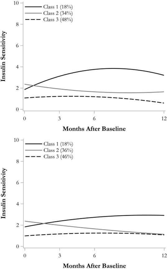
Plot of class-specific growth trajectories for 3-class solution of CPGMM from full data (N = 90; top panel) and from the data with outliers removed (N = 85; bottom panel)

Table 2.

Parameter estimates and class proportions for each class

Full data (N = 90)
Parameter	Class 1	Class 2	Class 3
Intercept	1.86	2.37	1.07
Linear slope	0.52	−0.18	0.08
Quadratic slope	−0.03	0.01	−0.01
Baseline variance	1.14	1.19	0.13
3-month variance	1.33	0.95	0.27
6-month variance	6.06	0.30	0.30
12-month variance	1.98	0.51	0.23
Residual correlation matrix	$\left[\begin{array}{cccc}\hfill 1\hfill & \hfill \hfill & \hfill \hfill & \hfill \hfill \\ \hfill .29\hfill & \hfill 1\hfill & \hfill \hfill & \hfill \hfill \\ \hfill .65\hfill & \hfill .75\hfill & \hfill 1\hfill & \hfill \hfill \\ \hfill .77\hfill & \hfill .60\hfill & \hfill .72\hfill & \hfill 1\hfill \end{array}\right]$	$\left[\begin{array}{cccc}\hfill 1\hfill & \hfill \hfill & \hfill \hfill & \hfill \hfill \\ \hfill .29\hfill & \hfill 1\hfill & \hfill \hfill & \hfill \hfill \\ \hfill .50\hfill & \hfill .17\hfill & \hfill 1\hfill & \hfill \hfill \\ \hfill .73\hfill & \hfill .40\hfill & \hfill .72\hfill & \hfill 1\hfill \end{array}\right]$	$\left[\begin{array}{cccc}\hfill 1\hfill & \hfill \hfill & \hfill \hfill & \hfill \hfill \\ \hfill .80\hfill & \hfill 1\hfill & \hfill \hfill & \hfill \hfill \\ \hfill .69\hfill & \hfill .85\hfill & \hfill 1\hfill & \hfill \hfill \\ \hfill .24\hfill & \hfill .64\hfill & \hfill .45\hfill & \hfill 1\hfill \end{array}\right]$
Class proportion	18%	34%	48%
Outliers removed (N = 85)
Intercept	1.84	2.38	0.99
Linear slope	0.21	−0.14	0.08
Quadratic slope	−0.011	0.003	−0.006
Baseline variance	0.53	0.97	0.08
3-month variance	0.71	0.84	0.21
6-month variance	1.99	0.39	0.24
12-month variance	0.78	0.35	0.26
Residual correlation matrix	$\left[\begin{array}{cccc}\hfill 1\hfill & \hfill \hfill & \hfill \hfill & \hfill \hfill \\ \hfill -.50\hfill & \hfill 1\hfill & \hfill \hfill & \hfill \hfill \\ \hfill .39\hfill & \hfill .22\hfill & \hfill 1\hfill & \hfill \hfill \\ \hfill .35\hfill & \hfill .44\hfill & \hfill .14\hfill & \hfill 1\hfill \end{array}\right]$	$\left[\begin{array}{cccc}\hfill 1\hfill & \hfill \hfill & \hfill \hfill & \hfill \hfill \\ \hfill .13\hfill & \hfill 1\hfill & \hfill \hfill & \hfill \hfill \\ \hfill .65\hfill & \hfill .29\hfill & \hfill 1\hfill & \hfill \hfill \\ \hfill .44\hfill & \hfill .83\hfill & \hfill .38\hfill & \hfill 1\hfill \end{array}\right]$	$\left[\begin{array}{cccc}\hfill 1\hfill & \hfill \hfill & \hfill \hfill & \hfill \hfill \\ \hfill .78\hfill & \hfill 1\hfill & \hfill \hfill & \hfill \hfill \\ \hfill .68\hfill & \hfill .78\hfill & \hfill 1\hfill & \hfill \hfill \\ \hfill .47\hfill & \hfill .79\hfill & \hfill .54\hfill & \hfill 1\hfill \end{array}\right]$
Class proportion	18%	36%	46%

A subtle but important feature of the model is that the covariance structure in each class can be uniquely estimated without issue. In GMMs, the covariance is difficult to estimate and often ends up constrained across classes as a casualty of the complex estimation, despite the fact that it rarely makes sense to force equality across latent classes. Figure 3 shows class growth trajectories and the empirical data of participants within each class to demonstrate the importance of allowing the covariance to be different across classes.

Fig. 3.

Class-specific growth trajectories plotted against the empirical data of people assigned to each class for full data (N = 90; top panel) and data with outliers removed (N = 85; bottom panel)

Class 1 clearly has more variability around its class trajectory, whereas Class 3 has little variability around its class trajectory. Constraining the variances to be equal across classes would clearly be inappropriate in this data. Though differences in variability are often overlooked and the focus is placed on the class growth trajectory, misspecifications in the covariance structure (such as inappropriate equality constraints across classes) adversely affect the class growth trajectories because misspecification in mixture models permeates to all parts of the model (Heggeseth & Jewell, 2013). This occurs because the model will classify participants in accordance with the specified covariance structure. If the covariance matrices were constrained to be equal across classes in these data, it is likely that many participants in Class 1 would be reclassified because they could not simultaneously be assigned to Class 1 while also satisfying the requirement that all classes have equal variability. Similarly, Class 3 likely would consume part of Class 2 if its variability were increased due to covariance equality constraints.

Note that although we use a marginal model in this analysis, the ability to answer the traditional research questions of interest with GMMs is unaffected. We were able to determine that there were multiple classes, and we estimated the growth trajectories for each class, just as is done with GMMs. Although not included here, the model can include variables to predict class membership or distal outcomes can be predicted by class membership (Peña et al., 2020). For instance, the empirical study from which these data originate collected additional risk factors and sociodemographic indicators which may help identify responders and non-responders.

Discussion

Assessing heterogeneity of growth trajectories with mixture models is a computationally intensive endeavor. However, the overreliance on the random effect modeling tradition in growth mixture models appears to unnecessarily exacerbate these complexities. The random effects tradition affords researchers little additional benefit with respect to answering common research questions of interests and frequently requires undesirable model alterations for the model to converge. This is especially true for the sample sizes encountered with typical randomized intervention studies, which even under the best circumstances, may fall far below growth mixture model recommendations.

Nonetheless, the established marginal modeling approach provides the basis for a solution to this issue. Marginal models are just beginning to be extended to include latent classes, and additional methodological research would be fruitful for more clearly delineating their strengths and weaknesses, but these models are theoretically more congruent with the typical goals of latent class analysis with repeated measures data in that they emphasize the growth trajectories in each class while accommodating the covariance as a secondary consideration. Though treating the covariance as ancillary may appear like a departure from the traditional growth mixture modeling framework, such secondary status is already on display with the common approach in growth mixture models of constraining all the covariance structures to be equal across classes. Only in a context where covariance structures were secondary would such an approach be permissible.

The covariance pattern growth mixture model merely takes the desire to accommodate—but not focus on—the covariance structure and places it in its natural home within the marginal model tradition. That is, if the main interest is differences between classes, there is no need to struggle with complex estimation associated with partitioning the within-class variability when these estimates are not of interest and not reported in most cases. Essentially, covariance pattern mixture models have the ability to improve convergence without sacrificing the quality of the model estimates or the ability to answer typical research questions.

References

- Bauer DJ, & Curran PJ (2003). Distributional assumptions of growth mixture models: Implications for overextraction of latent trajectory classes. Psychological Methods, 8, 338–363. [DOI] [PubMed] [Google Scholar]
- Bauer DJ, & Curran PJ (2004). The integration of continuous and discrete latent variable models: Potential problems and promising opportunities. Psychological Methods, 9, 3–29. [DOI] [PubMed] [Google Scholar]
- Biernacki C (2005). Testing for a global maximum of the likelihood. Journal of Computational & Graphical Statistics, 14, 657–674. [Google Scholar]
- Biernacki C, & Govaert G (1997). Using the classification likelihood to choose the number of clusters. Computing Science and Statistics, 29, 451–457. [Google Scholar]
- Burton P, Gurrin L, & Sly P (1998). Extending the simple linear regression model to account for correlated responses: An introduction to generalized estimating equations and multi-level mixed modelling. Statistics in Medicine, 17, 1261–1291. [DOI] [PubMed] [Google Scholar]
- Cook DI, Gebski VJ, & Keech AC (2004). Subgroup analysis in clinical trials. Medical Journal of Australia, 180, 289. [DOI] [PubMed] [Google Scholar]
- Cook RD, & Weisberg S (1982). Residuals and influence in regression. Chapman. [Google Scholar]
- Curran PJ, Obeidat K, & Losardo D (2010). Twelve frequently asked questions about growth curve modeling. Journal of Cognition and Development, 11, 121–136. [DOI] [PMC free article] [PubMed] [Google Scholar]
- Dayton CM, & Macready GB (1988). Concomitant-variable latent-class models. Journal of the American Statistical Association, 83, 173–178. [Google Scholar]
- Diallo TM, Morin AJ, & Lu H (2016). Impact of misspecifications of the latent variance covariance and residual matrices on the class enumeration accuracy of growth mixture models. Structural Equation Modeling, 23, 507–531. [Google Scholar]
- Diallo TM, Morin AJ, & Parker PD (2014). Statistical power of latent growth curve models to detect quadratic growth. Behavior Research Methods, 46, 357–371. [DOI] [PubMed] [Google Scholar]
- Diggle P, Heagerty P, Liang KY, & Zeger S (2002). Analysis of longitudinal data. Oxford University Press. [Google Scholar]
- Draper D (1995). Assessment and propagation of model uncertainty. Journal of the Royal Statistical Society: Series B, 57(1), 45–70. [Google Scholar]
- Firth J, Torous J, Nicholas J, Carney R, Pratap A, Rosenbaum S, & Sarris J (2017). The efficacy of smartphone-based mental health interventions for depressive symptoms: A meta-analysis of randomized controlled trials. World Psychiatry, 16, 287–298. [DOI] [PMC free article] [PubMed] [Google Scholar]
- Gardiner JC, Luo Z, & Roman LA (2009). Fixed effects, random effects and GEE: What are the differences? Statistics in Medicine, 28, 221–239. [DOI] [PubMed] [Google Scholar]
- Gilthorpe M, Dahly D, Tu Y, Kubzansky L, & Goodman E (2014). Challenges in modeling the random structure correctly in growth mixture models and the impact this has on model mixtures. Journal of Developmental Origins of Health and Disease, 5, 197–205. [DOI] [PMC free article] [PubMed] [Google Scholar]
- Goodman LA (1974). Exploratory latent structure analysis using both identifiable and unidentifiable models. Biometrika, 61, 215–231. [Google Scholar]
- Hanley JA, Negassa A, Edwardes MDD, & Forrester JE (2003). Statistical analysis of correlated data using generalized estimating equations: An orientation. American Journal of Epidemiology, 157, 364–375. [DOI] [PubMed] [Google Scholar]
- Hannan EJ, & Quinn BG (1979). The determination of the order of an autoregression. Journal of the Royal Statistical Society: Series B, 41, 190–195. [Google Scholar]
- Harring JR, & Hodis FA (2016). Mixture modeling: Applications in educational psychology. Educational Psychologist, 51, 354–367. [Google Scholar]
- Haymond MW (2003). Measuring insulin resistance: A task worth doing. But how? Pediatric Diabetes, 4, 115–118. [DOI] [PubMed] [Google Scholar]
- Heagerty PJ, & Zeger SL (2000). Marginalized multilevel models and likelihood inference. Statistical Science, 15, 1–26. [Google Scholar]
- Hedeker D, & Gibbons RD (2006). Longitudinal data analysis. Wiley. [Google Scholar]
- Heggeseth BC, & Jewell NP (2013). The impact of covariance misspecification in multivariate Gaussian mixtures on estimation and inference: An application to longitudinal modeling. Statistics in Medicine, 32, 2790–2803. [DOI] [PMC free article] [PubMed] [Google Scholar]
- Henderson NC, & Rathouz PJ (2018). AR (1) latent class models for longitudinal count data. Statistics in Medicine, 37, 4441–4456. [DOI] [PMC free article] [PubMed] [Google Scholar]
- Henson JM, Reise SP, & Kim KH (2007). Detecting mixtures from structural model differences using latent variable mixture modeling: A comparison of relative model fit statistics. Structural Equation Modeling, 14, 202–226. [Google Scholar]
- Hipp JR, & Bauer DJ (2006). Local solutions in the estimation of growth mixture models. Psychological methods, 11, 36–53. [DOI] [PubMed] [Google Scholar]
- Hubbard AE, Ahern J, Fleischer NL, Van der Laan M, Satariano SA, Jewell N, Bruckner T & Satariano WA (2010). To GEE or not to GEE: comparing population average and mixed models for estimating the associations between neighborhood risk factors and health. Epidemiology, 21, 467–474. [DOI] [PubMed] [Google Scholar]
- Huang FL (2016). Alternatives to multilevel modeling for the analysis of clustered data. The Journal of Experimental Education, 84, 175–196. [Google Scholar]
- Hurvich CM, & Tsai CL (1989). Regression and time series model selection in small samples. Biometrika, 76(2), 297–307. [Google Scholar]
- Imai K, & Ratkovic M (2013). Estimating treatment effect heterogeneity in randomized program evaluation. The Annals of Applied Statistics, 7, 443–470. [Google Scholar]
- Infurna FJ, & Grimm KJ (2018). The use of growth mixture modeling for studying resilience to major life stressors in adulthood and old age: Lessons for class size and identification and model selection. The Journals of Gerontology: Series B, 73, 148–159. [DOI] [PMC free article] [PubMed] [Google Scholar]
- Infurna FJ, & Jayawickreme E (2019). Fixing the growth illusion: New directions for research in resilience and posttraumatic growth. Current Directions in Psychological Science, 28, 152–158. [Google Scholar]
- Infurna FJ, & Luthar SS (2016). Resilience to major life stressors is not as common as thought. Perspectives on Psychological Science, 11, 175–194. [DOI] [PMC free article] [PubMed] [Google Scholar]
- Jedidi K, Jagpal HS, & DeSarbo WS (1997). Finite-mixture structural equation models for response-based segmentation and unobserved heterogeneity. Marketing Science, 16, 39–59. [Google Scholar]
- Jennrich RI, & Schluchter MD (1986). Unbalanced repeated-measures models with structured covariance matrices. Biometrics, 42, 805–820. [PubMed] [Google Scholar]
- Jo B, Finding RL, Wang CP, Hastie TJ, Youngstrom EA, Arnold LE, … & Horwitz SM (2017). Targeted use of growth mixture modeling: A learning perspective. Statistics in Medicine, 36, 671–686. [DOI] [PMC free article] [PubMed] [Google Scholar]
- Jo B, Wang CP, & Ialongo NS (2009). Using latent outcome trajectory classes in causal inference. Statistics and Its Interface, 2, 403–412. [DOI] [PMC free article] [PubMed] [Google Scholar]
- Jung T, & Wickrama KA (2008). An introduction to latent class growth analysis and growth mixture modeling. Social and Personality Psychology Compass, 2, 302–317. [Google Scholar]
- Kim S-Y (2012). Sample size requirements in single- and multiphase growth mixture models: A Monte Carlo simulation study. Structural Equation Modeling, 19, 457–476. [Google Scholar]
- Kooken J, McCoach DB, & Chafouleas SM (2019). The impact and interpretation of modeling residual noninvariance in growth mixture models. The Journal of Experimental Education, 87, 214–237. [Google Scholar]
- Kreuter F, & Muthén B (2008). Analyzing criminal trajectory profiles: Bridging multilevel and group-based approaches using growth mixture modeling. Journal of Quantitative Criminology, 24, 1–31. [Google Scholar]
- Laird NM, & Ware JH (1982). Random-effects models for longitudinal data. Biometrics, 38, 963–974. [PubMed] [Google Scholar]
- Lanza ST, & Cooper BR (2016). Latent class analysis for developmental research. Child Development Perspectives, 10, 59–64. [DOI] [PMC free article] [PubMed] [Google Scholar]
- Matsuda M, & DeFronzo RA (1999). Insulin sensitivity indices obtained from oral glucose tolerance testing: Comparison with the euglycemic insulin clamp. Diabetes Care, 22, 1462–1470. [DOI] [PubMed] [Google Scholar]
- McLachlan GJ, & Peel D (2004). Finite mixture models. Wiley. [Google Scholar]
- McNeish D, & Harring JR (2021). Improving convergence in growth mixture models without covariance structure constraints. Statistical Methods in Medical Research. 10.1177/0962280220981747 [DOI] [PubMed] [Google Scholar]
- McNeish D Harring JR, & Bauer DJ (2021). Nonconvergence, covariance constraints, and class enumeration in growth mixture models. PsyArXiv [DOI] [PubMed] [Google Scholar]
- McNeish D, & Harring JR (2020). Covariance pattern mixture models: Eliminating random effects to improve convergence and performance. Behavior Research Methods, 52, 947–979. [DOI] [PubMed] [Google Scholar]
- McNeish D, Stapleton LM, & Silverman RD (2017). On the unnecessary ubiquity of hierarchical linear modeling. Psychological Methods, 22, 114–140. [DOI] [PubMed] [Google Scholar]
- Muthén B, Brown CH, Masyn K, Jo B, Khoo ST, Yang CC, … & Liao J (2002). General growth mixture modeling for randomized preventive interventions. Biostatistics, 3, 459–475. [DOI] [PubMed] [Google Scholar]
- Muthén B, & Shedden K (1999). Finite mixture modeling with mixture outcomes using the EM algorithm. Biometrics, 55, 463–469. [DOI] [PubMed] [Google Scholar]
- Nagin DS (1999). Analyzing developmental trajectories: A semiparametric, group-based approach. Psychological Methods, 4, 139–157. [DOI] [PubMed] [Google Scholar]
- Nagin DS, & Tremblay RE (2005). Developmental trajectory groups: Fact or a useful statistical fiction?. Criminology, 43, 873–904. [Google Scholar]
- Northouse LL, Katapodi MC, Song L, Zhang L, & Mood DW (2010). Interventions with family caregivers of cancer patients: Meta-analysis of randomized trials. CA: A Cancer Journal for Clinicians, 60, 317–339. [DOI] [PMC free article] [PubMed] [Google Scholar]
- Nylund KL, Asparouhov T, & Muthén BO (2007). Deciding on the number of classes in latent class analysis and growth mixture modeling: A Monte Carlo simulation study. Structural Equation Modeling, 14, 535–569. [Google Scholar]
- Peña A, McNeish D, Ayers SL, Olson MLV, Wyst KB, Williams AN, & Shaibi GQ (2020). Response heterogeneity to lifestyle intervention among Latino adolescents. Pediatric Diabetes, 21, 1430–1436. [DOI] [PMC free article] [PubMed] [Google Scholar]
- Petras H, & Masyn K (2010). General growth mixture analysis with antecedents and consequences of change. In Piquero AR & Weisburd D (Eds.), Handbook of quantitative criminology (pp. 69–100). Springer. [Google Scholar]
- Pocock SJ, Assmann SE, Enos LE, & Kasten LE (2002). Subgroup analysis, covariate adjustment and baseline comparisons in clinical trial reporting: Current practice and problems. Statistics in Medicine, 21, 2917–2930. [DOI] [PubMed] [Google Scholar]
- Ryder JR, Kaizer AM, Jenkins TM, Kelly AS, Inge TH, & Shaibi GQ (2019). Heterogeneity in response to treatment of adolescents with severe obesity: The need for precision obesity medicine. Obesity, 27, 288–294. [DOI] [PMC free article] [PubMed] [Google Scholar]
- Sclove SL (1987). Application of model-selection criteria to some problems in multivariate analysis. Psychometrika, 52, 333–343. [Google Scholar]
- Schwarz G (1978). Estimating the dimension of a model. Annals of Statistics, 6, 461–464. [Google Scholar]
- Sijbrandij JJ, Hoekstra T, Almansa J, Reijneveld SA, & Bültmann U (2019). Identification of developmental trajectory classes: Comparing three latent class methods using simulated and real data. Advances in Life Course Research, 42, 100288. [DOI] [PubMed] [Google Scholar]
- Soltero EG, Konopken YP, Olson ML, Keller CS, Castro FG, Williams AN, … & Pimentel J (2017). Preventing diabetes in obese Latino youth with prediabetes: A study protocol for a randomized controlled trial. BMC Public Health, 17, 261. [DOI] [PMC free article] [PubMed] [Google Scholar]
- Tabák AG, Jokela M, Akbaraly TN, Brunner EJ, Kivimäki M, & Witte DR (2009). Trajectories of glycaemia, insulin sensitivity, and insulin secretion before diagnosis of type 2 diabetes: An analysis from the Whitehall II study. The Lancet, 373, 2215–2221. [DOI] [PMC free article] [PubMed] [Google Scholar]
- Tofighi D & Enders CK (2007). Identifying the correct number of classes in a growth mixture models. In Hancock GR, G.R. & Samuelson KM (Eds.), Advances in latent variable mixture models (p. 317–341). Greenwich, CT: Information Age. [Google Scholar]
- van De Schoot R, Sijbrandij M, Winter SD, Depaoli S, & Vermunt JK (2017). The GRoLTS-checklist: Guidelines for reporting on latent trajectory studies. Structural Equation Modeling, 24, 451–467. [Google Scholar]
- Verbeke G, & Lesaffre E (1996). A linear mixed-effects model with heterogeneity in the random-effects population. Journal of the American Statistical Association, 91, 217–221. [Google Scholar]
- Vermunt JK (2010). Latent class modeling with covariates: Two improved three-step approaches. Political Analysis, 18, 450–469. [Google Scholar]
- Wickrama KK, Lee TK, O’Neal CW, & Lorenz FO (2016). Higher-order growth curves and mixture modeling with Mplus: A practical guide. Routledge. [Google Scholar]
- Williams AN, Konopken YP, Keller CS, Castro FG, Arcoleo KJ, Barraza E, … & Shaibi GQ (2017). Culturally-grounded diabetes prevention program for obese Latino youth: Rationale, design, and methods. Contemporary Clinical Trials, 54, 68–76. [DOI] [PMC free article] [PubMed] [Google Scholar]
- Winkley K, Landau S, Eisler I, & Ismail K (2006). Psychological interventions to improve glycaemic control in patients with type 1 diabetes: Systematic review and meta-analysis of randomised controlled trials. BMJ, 333, 65. [DOI] [PMC free article] [PubMed] [Google Scholar]
- Zeger SL, Liang KY, & Albert PS (1988). Models for longitudinal data: A generalized estimating equation approach. Biometrics, 44, 1049–1060. [PubMed] [Google Scholar]
Associated Data
This section collects any data citations, data availability statements, or supplementary materials included in this article.