

Abstract
Little is known about whether exposure to unconventional oil and gas development is associated with higher mortality risks in the elderly and whether related air pollutants are exposure pathways. We studied a cohort of 15,198,496 Medicare beneficiaries (136,215,059 person-years) in all major U.S. unconventional exploration regions from 2001 to 2015. We gathered data from records of more than 2.5 million oil and gas wells. For each beneficiary’s ZIP code of residence and year in the cohort, we calculated a proximity-based and a downwind-based pollutant exposure. We analyzed the data using two methods: Cox proportional hazards model and Difference-in-Differences. We found evidence of statistically significant higher mortality risk associated with living in proximity to and downwind of unconventional oil and gas wells. Our results suggest that primary air pollutants sourced from unconventional oil and gas exploration can be a major exposure pathway with adverse health effects in the elderly.
Introduction
Oil and natural gas development from low-permeability geological formations (known as Unconventional Oil and Gas Development [UOGD]) has rapidly expanded over the past decade. As of 2015, more than 100,000 onshore UOGD wells have been drilled using directional drilling combined with multi-stage high-volume hydraulic fracturing (fracking).1 17.6 million U.S. residents currently live within one kilometer of at least one active well.2 The annual percent of newly completed oil and gas wells that target unconventional formations increased from 2.3% in 2001 to 47% in 2015, and then to 71% in 2019. Compared with Conventional Oil and Gas Development (COGD), UOGD generally involves longer construction periods, larger well pads, and requires larger volumes of water, proppants, and chemicals during the multi-stage hydraulic fracturing process.3 Due to the rate of expansion and larger theoretical environmental impacts, it is critical to study the health effects and exposure pathway(s) of UOGD.
UOGD activities – including pad construction, well drilling, hydraulic fracturing, and production – have been associated with increased human exposure to harmful agents.4–7 UOGD-related primary air contaminants include Volatile Organic Compounds (VOCs),8 nitrogen oxides,9 and naturally occurring radioactive materials.10,11 UOGD operations have also been associated with elevated concentrations of organic compounds,12 chloride, and total suspended solids in drinking water.13 Higher levels of UOGD-associated non-chemical exposures, such as noise14 and night light,15 have also been reported in nearby neighborhoods. Previous health effects studies have found significant associations between proximity-based exposure to UOGD and adverse prenatal,16–19 respiratory,20 cardiovascular,21 and carcinogenic outcomes.22
The association between exposure to UOGD and all-cause mortality among the elderly has not been quantified. Additionally, previous studies were conducted in specific geographical locations and thus did not evaluate heterogeneity in exposures and outcomes across large geographical regions. Previous studies also did not investigate the exposure pathway(s) through which UOGD activities could lead to adverse health effects, primarily due to a lack of large-scale measurement of UOGD-sourced pollutants in some intensively drilled regions. To address these gaps in the data and characterize the spatiotemporal gradients of the UOGD-sourced agents, investigators have designed Proximity-based Exposure metrics (PEs) of varying complexity.23 Most of these PEs assumed a uniform distance decay in the concentrations of UOGD-related agents in all directions. Although this assumption largely holds for noise and light pollution, which travel similarly in all directions, it does not account for the directional dispersion of UOGD-sourced airborne or waterborne pollutants in nearby environments. PE metrics could be improved by incorporating the transport mechanisms of UOGD-sourced agents, such as wind direction and underground water flow.24 Accounting for the directional dispersion of agents would also enable investigation of potential exposure pathways.
We, following the process of Figure 1, built an open cohort of 15,198,496 Medicare beneficiaries (136,215,059 person-years) residing in our study area (Figure 2), which includes all major U.S. UOGD regions (Supplementary Note 1) from 2001 to 2015. We also gathered location, construction, and production records for more than 2.5 million oil and gas wells. Rather than solely relying on PE, we calculated Downwind-based Exposure metrics (DE), which incorporate wind direction in the exposure assessment (Figure 3). Based on these two exposure metrics (PE and DE), we conducted two sets of analyses (Analysis Set I and II) to investigate whether living in proximity to and downwind of UOGD wells is associated with higher mortality risks in Medicare beneficiaries. For Analysis Set I, we used a Cox proportional hazards model including PE only (Model I) or both PE and DE (Model II); for Analysis Set II, we relied on two quasi-experimental designs: Difference in Differences (DiD) and Difference in Difference in Differences (DDD). The results of both analyses provide additional evidence about the robustness of our main results against different model specifications.
Figure 1.
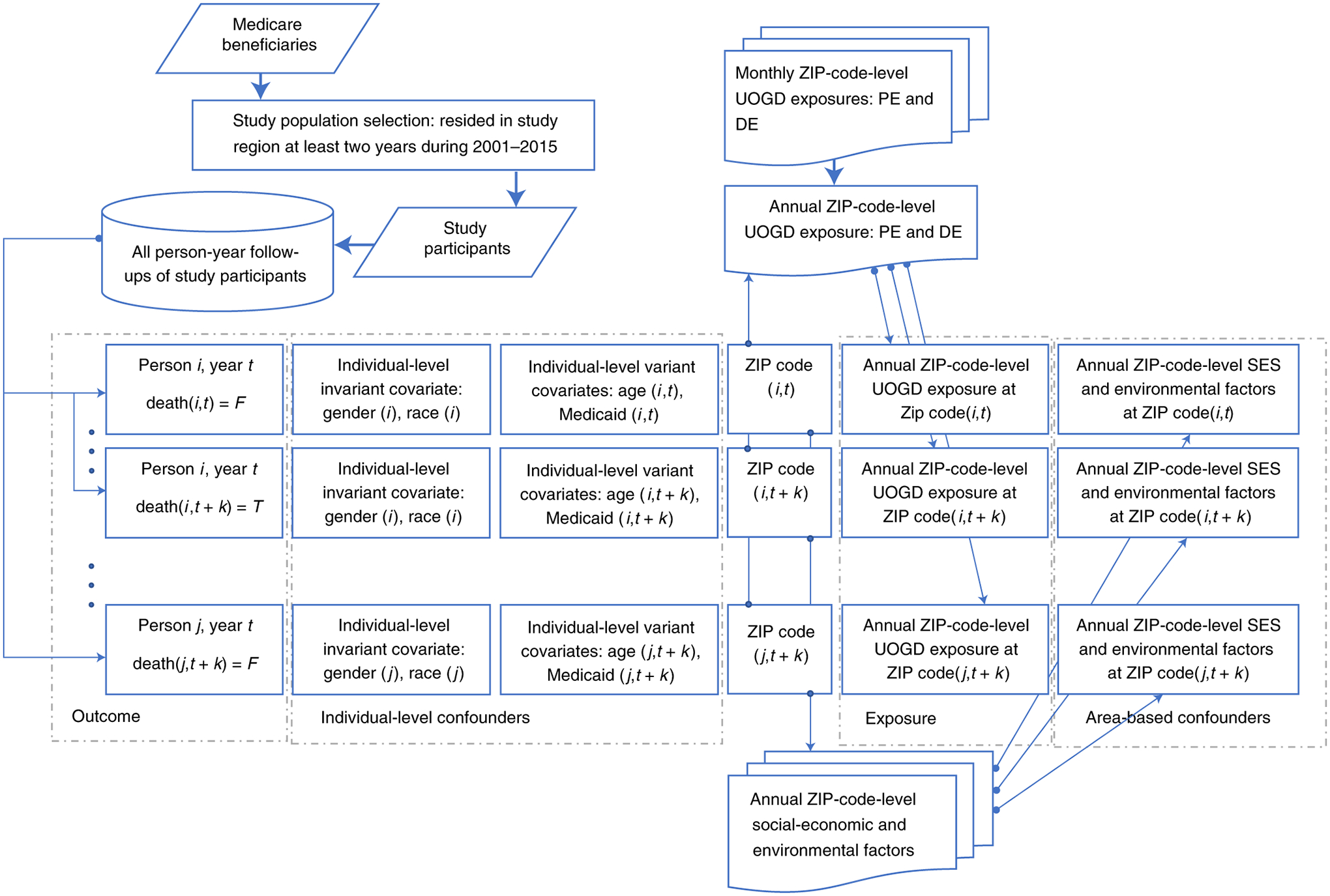
Process diagram of our study design.
We obtained mortality information of all Medicare enrollees and then selected those residing in the study region. For each person-year of follow-up, we extracted data on the occurrence of death, individual-level covariates, and the ZIP code of residence. The ZIP code of residence may have changed if the participant moved out of the original ZIP code. We calculated monthly UOGD exposures (PE and DE) based on Enverus™ database and monthly prevailing wind direction data. These monthly exposures were aggregated by year. Using the ZIP code for each person-year, the area of UOGD exposures (PE and DE) could be linked to individual records. Other area-based potential confounders such as socioeconomic factors and air pollutant levels could also be linked to the records.
Figure 2.
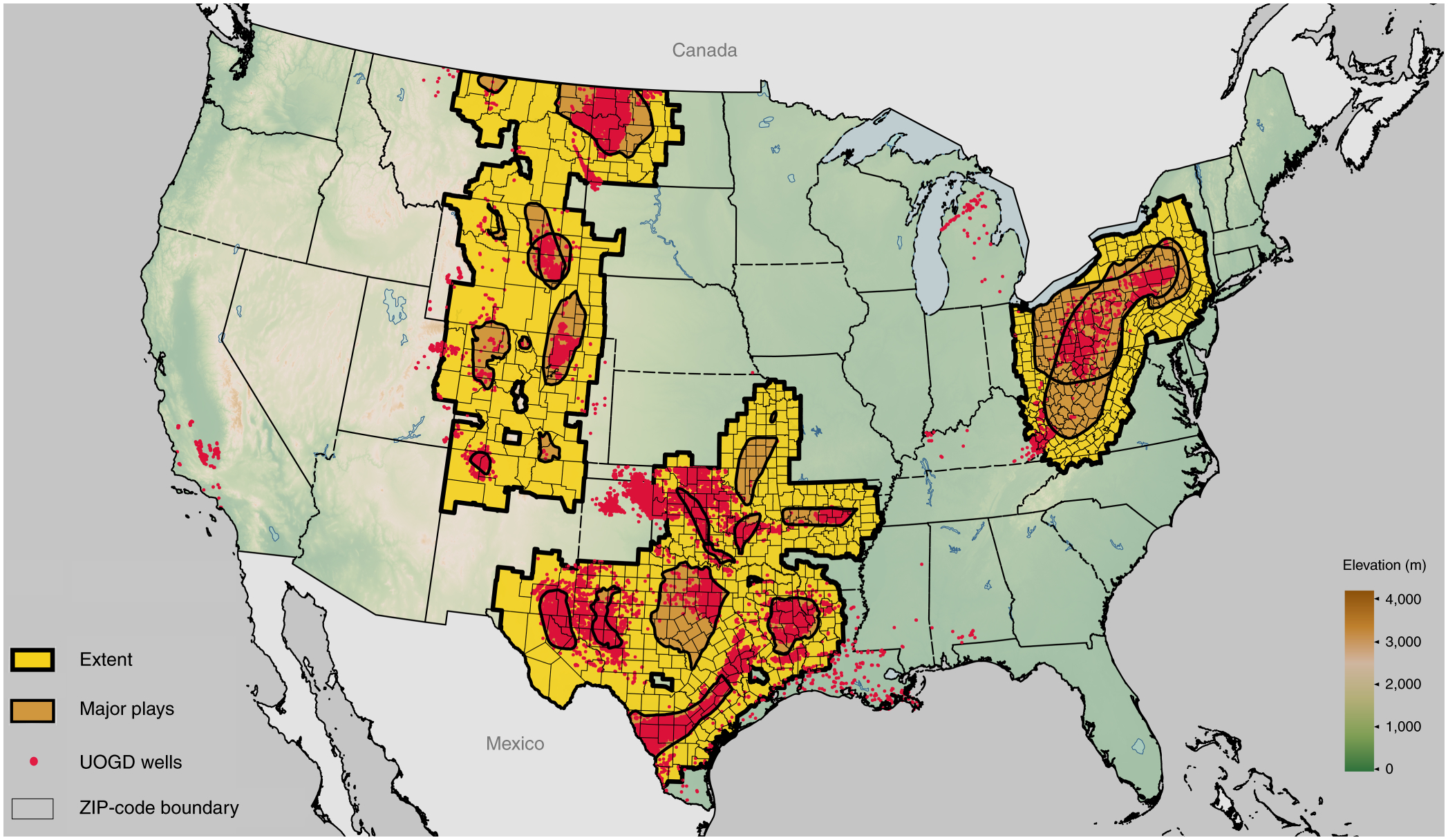
Map of the study area, which contains more than 120,000 active UOGD wells located in 9,244 ZIP codes as of December 2015.
The study area was grouped into three subregions for subregional analysis. The northern subregion covers the Bakken and Niobrara formations. The eastern subregion covers the Marcellus and Utica formations. The southern subregion covers the Permian, Barnett, Eagle Ford, Haynesville, Woodford, and Fayetteville formations.
Figure 3.
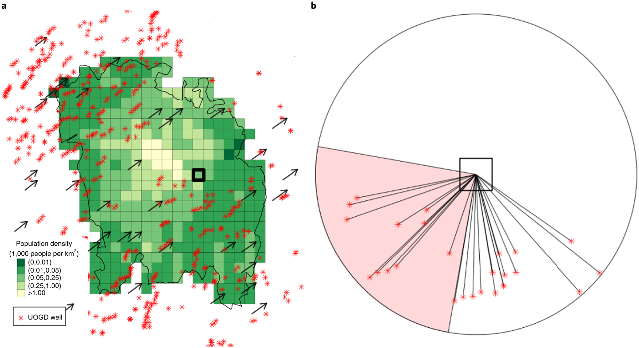
UOGD exposure assessment in an example ZIP code and month (Washington, Pennsylvania, 15301, August 2015).
Panel A shows the locations of active UOGD wells, the 1×1 km grid population density, and prevailing monthly wind direction. Panel B illustrates the calculation of PE and DE for an example grid in the ZIP code, which is bolded in Panel A. Proximity-based UOGD exposure (PE= IDWall) was calculated as the IDW of wells in all directions within a circular buffer* and was used in Model I. The UOGD exposure contributed by upwind wells (IDWup) was calculated using the IDW of all wells that fall within the windward circular quadrant. The ratio between IDWup and IDWall was defined as downwind exposure (DE+) and was used in Model II.
* The radius of the circular buffer is 5 km for illustration purposes.
Spatiotemporal patterns of mortality exposure and covariates
We observed a declining trend in all-cause mortality of Medicare beneficiaries across three subregions during our study period (2001–2015) (Supplementary Table 1). During this same period, a total of 174,624 UOGD wells were completed, which increased PE in all three subregions (Supplementary Figure 1 and Supplementary Note 2). Table 1 summarizes key covariates by PE and DE levels. For the demographic variables, each of the four UOGD PE levels had a lower percentage of female and white beneficiaries, younger age beneficiaries, and a higher percentage of beneficiaries with Medicaid eligibility, compared to the unexposed level. For the environmental factors, each of the four UOGD PE levels had lower PM2.5 concentrations and were less developed, compared to the unexposed level. For the socioeconomic factors, each of the UOGD PE levels had a lower population density and higher percentage of residents without a high school diploma, compared to the unexposed level. Of note, the values of all these covariates were similar when we compared DE+ (downwind) versus DE− (upwind) subgroups within each PE level (Table 1).
Table 1.
Characteristics of population grouped by PE and DE to UOGD.
Continuous PE was categorized by three PE percentiles: 25th percentile (0.03), 50th percentile (0.21), and 75th percentile (1.71) into four levels. These four levels approximately correspond to living relatively far away from UOGD (Low-PE), living around the ZIP Code where scattered UOGD exists (Med-Low-PE), living within the ZIP Code where scattered UOGD happens or living around the ZIP Code where dense UOGD exists (Med-High-PE), and living within a ZIP Code where dense UOGD exists (High PE). DE+ indicates the downwind sub-level and DE− indicates the upwind sub-level.
| No-PE* | Low-PE | Med-Low-PE | Med-High-PE | High-PE | |||||
|---|---|---|---|---|---|---|---|---|---|
| -- | DE− | DE− | DE− | DE− | |||||
| No. of Beneficiaries | 13,176,937 | 1,221,558 | 1,333,627 | 1,131,319 | 753,219 | ||||
| No. of Person-years | 110,093,570 | 4,321,587 | 4,273,579 | 3,687,253 | 3,236,837 | ||||
| No. of Deaths | 5,434,451 | 214,430 | 127,428 | 211,834 | 185,160 | 154,964 | |||
| Mortality (%) | 4.9 | 5.0 | 5.0 | 5.0 | 4.8 | ||||
| Individual level factors | |||||||||
| Female (%)§ | 57.6 | 56.4 | 56.6 | 56.5 | 56.1 | ||||
| White (%) | 90.7 | 91.7 | 88.2 | 90.2 | 89.6 | ||||
| Medicaid Eligibility (%) | 10 | 12.2 | 13.3 | 12.1 | 11 | ||||
| Age (year) | 75.1±7.6 | 74.8±7.5 | 74.8±7.5 | 74.9±7.5 | 74.6±7.5 | ||||
| ZIP Code-level environmental covariates | |||||||||
| PE of COGD | 5.0±14.0 | 12.0±19.9 | 12.8±19.9 | 20.2±25.2 | 15.4±25.7 | ||||
| PM2.5 (μg/m3) | 10.3±2.7 | 8.9±2.6 | 9.1±2.3 | 9.3±2.1 | 9.3±1.6 | ||||
| Development Ratio (%)‡ | 40.8±33.7 | 16.9±21.9 | 27.3±31.5 | 24.1±27.6 | 31.3±30.9 | ||||
| ZIP Code-level socioeconomic covariates | |||||||||
| Pop Density (100 person/km2) | 17.7±25.9 | 4.6± 8.8 | 9.6±15.7 | 7.7±12.1 | 10.8±13.9 | ||||
| Mean Household Income (×103 $) | 25.0±13.8 | 25.7±13.2 | 27.2±15.5 | 25.6±13.0 | 22.3±12.9 | ||||
| No High School (%) | 8.2±5.8 | 9.7±5.5 | 10.4±7.2 | 9.6±5.8 | 8.8±5.8 | ||||
| County level behavioral risk covariates | |||||||||
| BMI* | 27.0±1.0 | 27.4±1.2 | 27.5±1.1 | 27.5±1.0 | 27.4±1.2 | ||||
| Non-Smoker (%) | 46.9±6.5 | 46.7±8.0 | 44.9±8.7 | 46.6±7.4 | 43.9±7.4 | ||||
Individual-level categorical covariates are reported as a percentage.
Individual-level numeric covariates are reported as a mean ± standard deviation.
ZIP Code-level covariates are reported as mean ± standard deviation.
Development ratio is calculated as the percent of land in a ZIP Code developed for residential and industrial use.
BMI denotes body-mass index (the weight in kilograms divided by the square of the height in meters).
Association between living proximity to UOGD and mortality risk
In Model I of Analysis Set I (Cox proportional hazards model, PE only), exposure to each of the four PE levels was associated with a statistically significant increase in mortality risk compared to the unexposed level (Figure 4A and Supplementary Table 2). The estimated risk of mortality increased monotonically when the PE level increased from low to high (Figure 4A). A high PE level was associated with a significantly elevated risk of all-cause mortality (HR: 1.025; 95% confidence interval [CI]: 1.021 to 1.029). According to the results of DiD analysis of Analysis Set II, the point estimate of a two-way interaction between “treatment” (high and medium-high PE vs medium-low and low PE) and “intervention” (pre- or post-drilling) was 0.19% [95% CI: 0.12%–0.27%, p< 0.001] indicating that the pre- and post-drilling difference in the likelihood of death was significantly higher in high and medium-high PE communities than in low and medium-low PE communities. Details about both sets of analyses are described in Methods section. The model parameters for Analysis Set I (Cox proportional hazards model) and Analysis Set II (DiD) represent different estimands, which led to the difference in magnitude between the two sets of results. The two Analysis Sets also used different comparison groups and exposure assessment methods. More specifically, the results of Analysis Set I quantified the proportional increase in the mortality risk (hazard ratio) when comparing communities at any of the four PE levels (low, medium-low, medium-high, and high) versus an unexposed community, whereas the results of Analysis Set II quantified the absolute difference in mortality risks pre- versus post-drilling for the high and medium-high PE communities versus medium-low and low PE communities.
Figure 4.
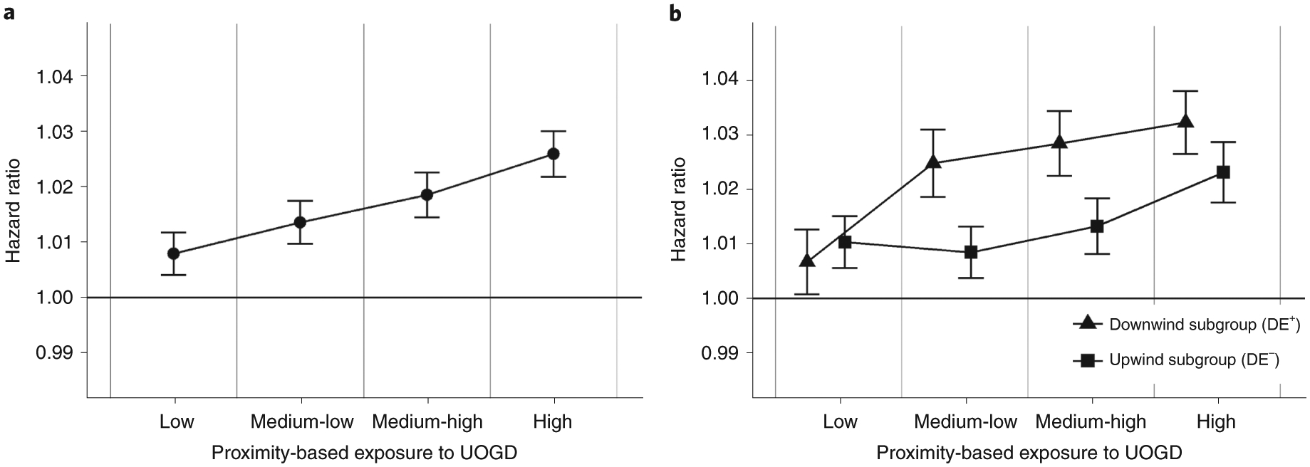
The results of Model I and Model II in Analysis Set I.
Estimated relative risk of mortality, which is represented by the point estimate of the hazard ratio (HR, center point) and its 95% confidence interval (bar) associated with each level of proximity-based exposure to UOGD (PE) and subgroups of up- or downwind exposure to UOGD (DE) within each PE level. Each PE level of exposure (low, medium-low, medium-high, and high) and each subgroup of DE exposure (DE+ or DE−) was compared to the unexposed level. The unexposed level was defined as person-years for individuals whose residential addresses are distant from UOGD and COGD. Panel A shows the result from the Model I analysis, which investigated the relative risk of mortality associated with each PE level when compared to the unexposed level. Panel B shows the result from the Model II analysis, which investigated the association between PE and all-cause mortality in the DE+ and DE− subgroups. We then compared the relative risks associated with the DE+ subgroup and DE− subgroup within each PE level using a t-test.
Association between living downwind to UOGD and mortality risk
For Model II of Analysis Set I (Cox proportional hazards model, PE and DE), a t-test revealed that living downwind of UOGD wells is associated with a higher risk of death compared to living upwind of UOGD (Figure 4B and Supplementary Table 2). Specifically, within the high PE group, we found a significant increase in mortality risk when comparing the downwind subgroup (DE+) with the unexposed group (HR 1.031; 95% CI: 1.025 to 1.037) and when comparing the upwind subgroup (DE−) with the unexposed group (HR 1.022; 95% CI: 1.017 to 1.028). Importantly, for the high PE group, we found that estimated HR for the downwind (DE+) subgroup is significantly higher than the estimated HR for the upwind (DE−) subgroup, with a difference in mortality risk equal to 0.009 (95% CI: 0.003 to 0.014, p<0.001). In the medium-high PE group, the difference in mortality risk between the DE+ and DE− subgroups was 0.015 (95% CI: 0.009 to 0.020, p<0.001); in the medium-low PE level, the difference was 0.016 (95% CI: 0.01 to 0.022, p<0.001) (Supplementary Table 2). We observed a distance decay of estimated mortality risk in both the upwind and downwind directions. The distance decay in the downwind direction was slower than that in upwind direction. A DDD analysis of Analysis Set II revealed that the point estimate of a three-way interaction between treatment, intervention, and wind is 0.68% (95% CI: 0.53%–0.83%, p<0.001), suggesting that the DiD estimates in communities mostly downwind of UOGD activities is greater than the DiD estimates in communities mostly upwind of UOGD activities. The results for both Analysis Sets, using Cox proportional hazards Model II and DDD, are consistent despite the difference in magnitude.
Results of subgroup, subregional, sensitivity and robustness analysis
According to the results of subgroup analysis by demographics in Analysis Set I, the estimated mortality risks in the female subgroups were greater than in the male subgroups within each PE level (Supplementary Figure 2A). In addition, the wind-dependent difference was more obvious in male and younger subgroups compared to female and older subgroups (Supplementary Figure 2E–H). The results of subregional analyses showed similar associations between UOGD exposure, both PE and DE, and all-cause mortality across the three subregions (Supplementary Table 3).
Based on a sensitivity analysis, the associations we found in Analysis Set I were not sensitive to the cut points selected for PE categorization (Supplementary Figures 3 and 4). Using the modified Model I shown in Supplementary Figures 5A, 6A, and 7A, the estimated risks associated with PE levels were sensitive to omitting ZIP code-level environmental and socioeconomic covariates. However, wind-dependent differences in the estimated HRs assessed via the t-test from Model II were not sensitive to the omission of these covariates (Supplementary Figures 5B, 6B, and 7B). Not adjusting for COGD exposure in Model I and Model II led to higher estimated HRs but revealed significant wind-dependent differences (Supplementary Figure 8). Our results did not change remarkably when we did not adjust for PM2.5 (Supplementary Table 4). Overall, the results of the t-test following Model II did not vary when we omitted these two covariates. We conducted further sensitivity analyses to unmeasured confounding by calculating the E-values for the results of Model I.25,26 The results suggest that the conclusions of Model I are overall robust to unmeasured confounding bias (Supplementary Table 5).
To justify the parallel trend assumption for the DiD analysis in Analysis Set II, we calculated annual mortality rates for the treatment group (high and medium-high PE) and the comparison group (medium-low and low PE). We centered the annual mortality rates by the ZIP code-specific drilling time (Figure 5), such that negative values indicate the pre-drilling period and positive values indicate the post-drilling period. We observed similar pre-drilling trends in mortality that diverged post-drilling, confirming the validity of the parallel trend assumption. Moreover, we conducted a pre-test with an event-study regression,27 which included four lead and four lag terms of the ZIP code-specific drilling time (Supplementary Note 9). As shown in Figure 6, all four coefficients for the lead terms were not statistically significantly greater than zero, suggesting no pre-drilling difference in mortality. The coefficients of all four lag terms were significantly greater than zero, suggesting that UOGD activities have a long-term influence on mortality post-drilling.
Figure 5.
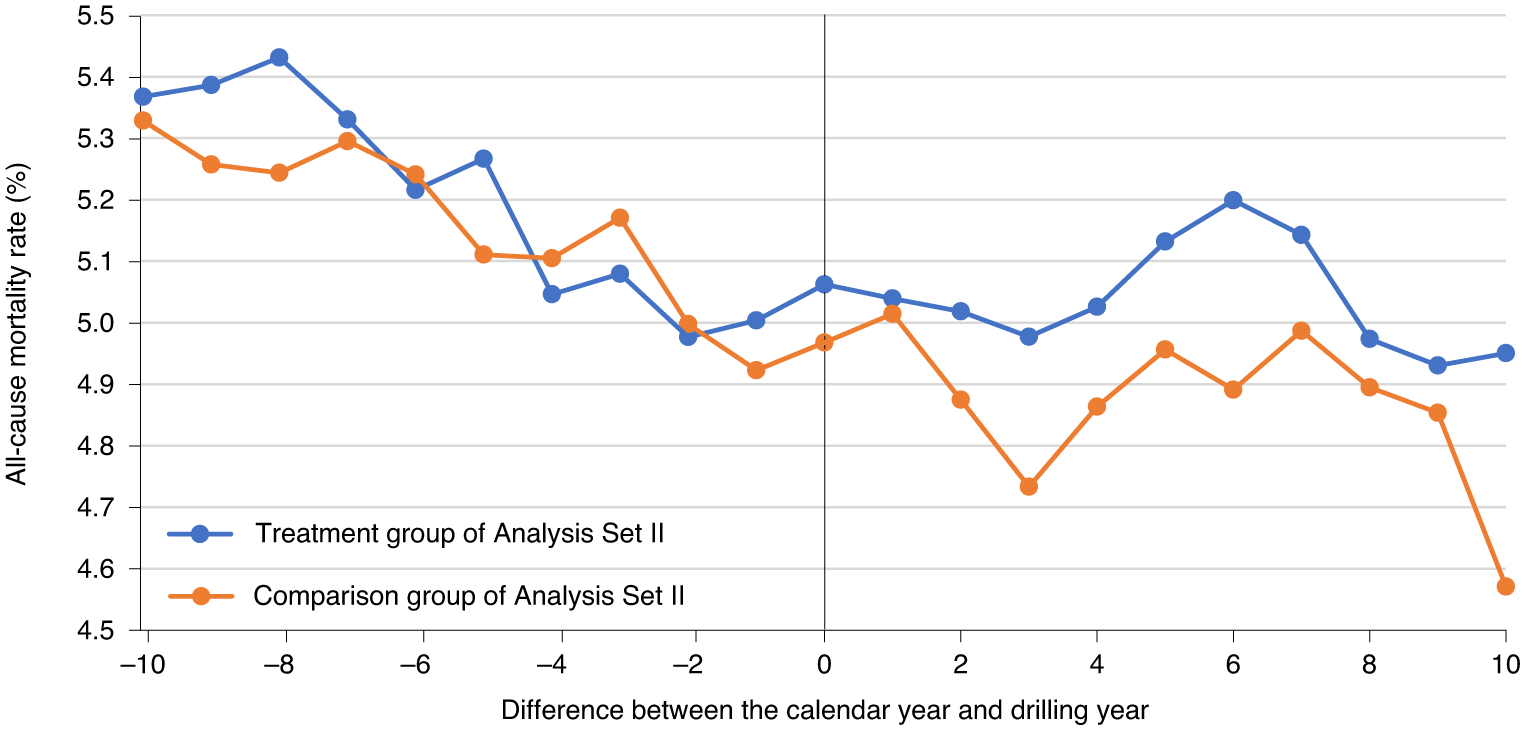
Trends in all-cause mortality rate in the treatment group and comparison group pre- and post-drilling.
Figure 6.
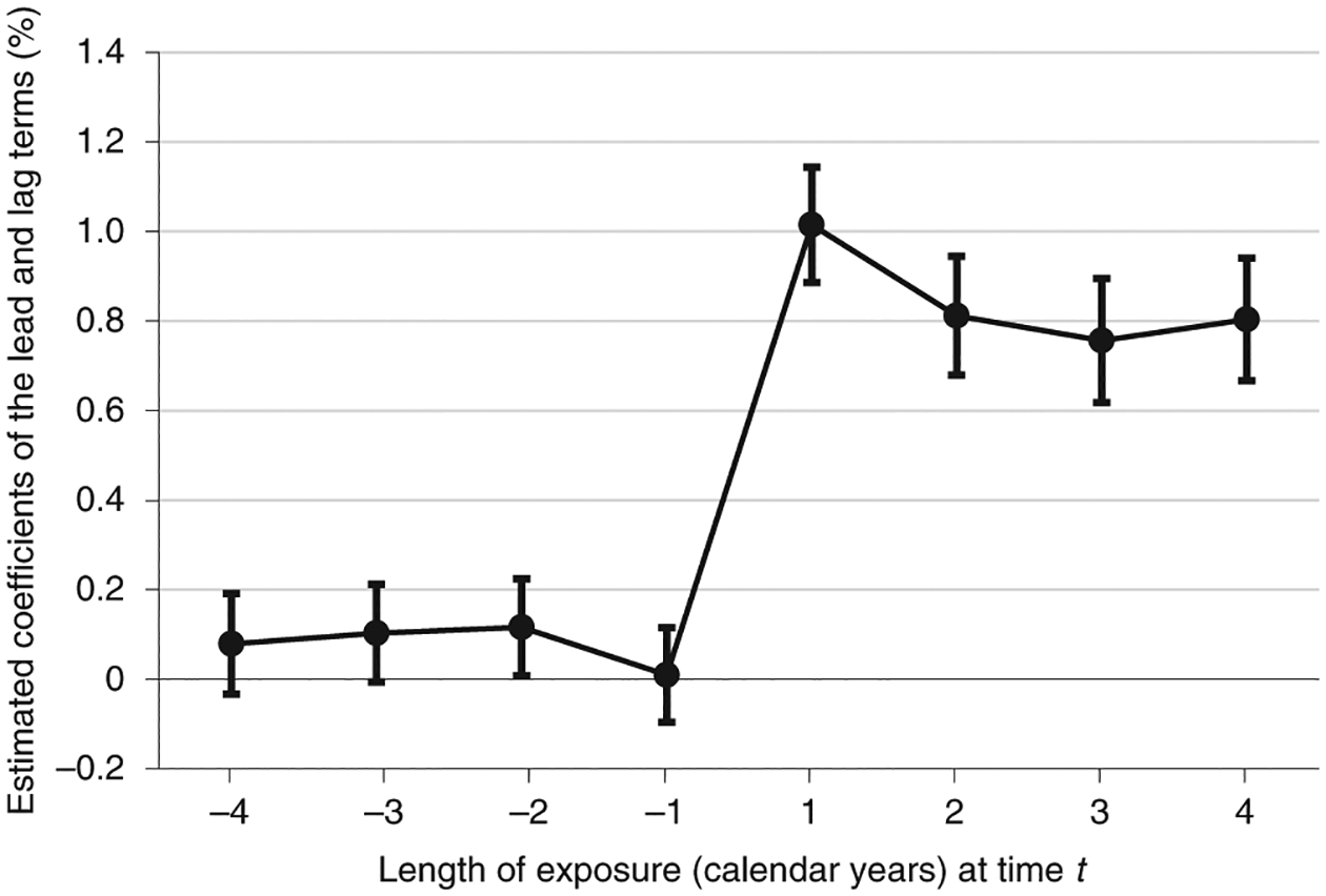
The results of a pre-test of the assumption of parallel trends in the mortality rate between the treatment and comparison groups (DiD in Analysis Set II). Negative values on the x-axis (length of exposure) indicate lead terms and positive values indicate lag terms with respect to drilling time. The point estimates of the lead and lag terms are presented; 95% confidence intervals for each estimate are shown as error bars.
Discussion
We found evidence of a statistically significant association between residential exposure to UOGD, characterized by PE and DE exposure metrics, and relative risk of all-cause mortality in a large cohort of Medicare beneficiaries. The significant wind-dependent differences in the estimated mortality risks within each of the four PE levels suggested that primary airborne pollutants emitted by UOGD activities might represent a key exposure pathway. These associations were observed in all three subregions (Supplementary Table S3), both genders, all age groups, and both major races (Supplementary Figure 2). These findings indicate that the extensive expansion of onshore UOGD in the past decade has impacted the health of Medicare beneficiaries living in nearby communities when adjusted by socioeconomic, environmental, and demographic factors.
Participants living in proximity to UOGD are exposed to diverse chemical and physical pollutants. We recognized that proximity-based exposure, such as the PE we constructed, assumes a uniform distance-decay gradient of UOGD exposure in all directions and does not account for transport mechanisms. To address this limitation, we calculated DE+ and DE− subgroups within each PE level to study the role of wind direction, attempting to isolate the impact of agents transported by air. We found that, within each PE level above Low, the mortality risks associated with the DE+ subgroup (downwind) are statistically significantly higher than those associated with the DE− subgroup (upwind) when both were compared to the unexposed group (Supplementary Tables 2). These results suggest that airborne contaminants emitted by UOGD and transported downwind contribute to increased mortality. We also found statistically significant, but lower relative risk, for populations residing upwind of UOGD wells. We hypothesized that these associations could be due to other agents whose transport are independent of atmospheric movement, such as surface and groundwater contaminants, traffic-dependent impacts, noise, light pollution, and lifestyle disruption. These associations could also be explained by UOGD-related airborne pollutants transported to upwind communities but at a lower frequency than to downwind communities.
In previous observational UOGD health effect studies, a primary challenge was that the study population could not be randomly assigned to exposed and unexposed groups, suggesting that people who live closer to UOGD have different initial health conditions (likely due to different socioeconomic status) from those living further away from UOGD operations. Observational studies based solely on proximity-based exposure metrics are vulnerable to unobserved confounding factors bias – a key limitation in previous studies and in the Model I of Analysis Set I.28 To address this limitation, we accounted for wind direction when estimating exposure. We hypothesized that the estimation of a downwind-upwind difference in mortality risk within a PE level is less likely to be affected by confounding bias because of similar baseline values (Table 1). Furthermore, when we used a t-test to compare the mortality risks in the downwind subgroup (DE+) versus the upwind subgroup (DE−) within the same PE level, the results were robust to the omission of socioeconomic and environmental confounding factors (Supplementary Figures 5–8).
Additionally, we conducted a sensitivity analysis to unmeasured confounding bias by calculating the evidence-values of the results of Model I of Analysis Set I.25,26 We found that the evidence-value of the HR ratio associated with high PE level is 1.19 (Supplementary Table 5). This means that to nullify the reported association between UOGD proximity and mortality, an unmeasured confounder would need to be associated with both UOGD proximity and mortality by a HR of 1.19, after accounting for all the measured confounders. Considering the very large value of this HR for the unmeasured confounder, such a situation is very unlikely.
We conducted two sets of analyses to investigate the association between exposure to UOGD and mortality. Model I and Model II of Analysis Set I are traditional regression models. DiD and DDD of Analysis Set II are quasi-experimental designs. DiD and DDD have an advantage that — under the assumption of parallel trends — the conclusions are less sensitive to unmeasured confounding bias.29 Despite differences between the two Analysis Sets and the models used, they aim to qualitatively address the same question: whether living in proximity to and downwind of UOGD wells is associated with a higher mortality risk. Finding consistent results with these two sets of approaches provides evidence that our conclusions are robust with respect to different study designs, choice of comparison groups, and specifications for the statistical model used.
Our study relied on a nationwide cohort of over 15 million Medicare beneficiaries. Medicare beneficiaries include more than 95% of U.S. citizens 65 years of age or older. Our study population is nationally representative and has a low influence of occupational UOGD exposure. This cohort was first followed in 2001, prior to the widespread UOGD expansion. We also gathered data from a comprehensive database covering more than 2.5 million oil and gas wells. The geographic coverage encompasses all shales, and allowed us to analyze national and regional associations with mortality risk. Previous regional studies did not examine the regional heterogeneity of observed associations. Our subregional analysis could be regarded as three independently conducted epidemiology studies of the association based on an identical exposure-outcome pair.
Our study has several limitations. First, we were unable to estimate associations between specific UOGD-related airborne agent(s) and mortality due to unavailability of high-resolution exposure data of air pollutants other than PM2.5. Therefore, our results should be cautiously interpreted as the mortality risk associated with an air pollutant mix originating from UOGD wells. Further observational studies near UOGD, especially in both wind directions, are necessary to identify the air pollutant(s) responsible for the health effects observed in this study. Second, we were not able to account for well characteristics including drilling depth, product type, well age, productivity, operator, and wastewater management method in our exposure assessment due to a lack of information for all domestic major shales. As a result, we could not apply the most advanced PE metric that incorporates diverse secondary information in our national study.23 A more comprehensive nationwide UOGD dataset may address this limitation and enable us to estimate the relative contribution of each section of UOGD activities. Third, we had available data on ZIP code-level but not street-level address of residence. This could result in potential exposure misclassification; however, we used a population-weighted method to mitigate this issue.
Considering the increased rate and scale of UOGD expansion, it is critical to understand the potential health risks associated with this industry. In this study, we designed two metrics and employed them in multiple models to estimate the health effects of living proximity and downwind of UOGD wells, respectively. According to our models, we conclude that residential exposure to UOGD is positively associated with an elevated risk of all-cause mortality in the Medicare population and airborne contaminants represent a key exposure pathway.
Methods
We conducted a nationwide study to estimate the association between exposure to UOGD and mortality risk among Medicare beneficiaries. We hypothesized that mortality risks are higher for individuals who live in proximity to and downwind from UOGD activities due to the directional transport of UOGD-sourced primary airborne pollutants. To test this hypothesis, we computed PEs with a traditional approach and then computed DE to UOGD by incorporating wind direction into PE. We quantified the wind-dependent difference in UOGD-associated mortality impacts using PEs and DEs to advance our understanding of whether UOGD-sourced air pollutants are significant exposure pathways.
Mortality Data
Our study area (Figure 2) includes all Medicare beneficiaries who live in ZIP codes within or around seven major shales defined by the U.S. Energy Information Administration.30 The Medicare beneficiaries denominator file was obtained from the Center for Medicare and Medicaid Service.31 We grouped ZIP codes into three non-adjacent subregions: northern, eastern, and southern, and then built an open cohort with person-years of follow-up for Medicare beneficiaries 65 or older at enrollment who lived in a ZIP code included in the study area for at least one year from 2001 to 2015. For each person-year of follow-up, we extracted individual age, race, sex, Medicaid eligibility, place of residence within the ZIP code, and date of death. The study design is summarized in Figure 3.
UOGD Data
We obtained location, construction, and production information for domestic oil and gas wells with production records during 2001 to 2015 from the Enverus™ (formerly Drillinginfo.com) Direct Access Service.32 Enverus™ aggregates the information reported by state energy agencies and maintains a national database used by the U.S. Energy Information Administration for its Monthly Energy Review. All oil and gas wells are classified in the Enverus™ database into horizontal, vertical, or directional wells, or those missing drilling type information. We categorized horizontally drilled wells as UOGD and vertically drilled wells as COGD;3 we categorized wells missing drilling type information using a random forest prediction model detailed in Supplementary Note 6. According to Supplementary Figure 9, the most important predictors in the random forest model are the drilling type of neighboring wells. Wells under construction or in production were considered active and included in the exposure metric calculation. We used annual subregional average construction duration to impute missing construction length for wells with a production history but without construction records.
Exposure Assessment
For each Medicare beneficiary, we calculated the individual-level exposure to UOGD for each year of follow-up at their ZIP code of residence. We calculated PE using an inverse-distance-weighting method without incorporating wind information. Specifically, for each individual-level ZIP code of residence, we identified all 1-km grid cells and the corresponding population density obtained from Gridded Population of the World, Version 4 (GPWv4).33 Then we calculated the distances between grid centers and each active UOGD well within a 15-km circular buffer by month for each 1-km grid cell (Figure 3A). Next, we calculated grid-specific PE by summing the inverse of these distances, as shown in the Figure 3 formulas. In the Medicare cohort, the spatial resolution of residential location information is at the ZIP code level. As a result, we calculated ZIP code-level PE by taking a weighted average of grid-level PE according to grid-level population density. This population-weighted aggregation enabled us to control for the uneven distribution of residents within a ZIP code (Figure 3A), which reduced exposure misclassification, especially in sparsely populated rural areas. We took the annual average of the monthly PE values and assigned an annual ZIP code-level PE to each participant in the ZIP code in the year of follow-up. In summary, our PE metric incorporated: 1) the time an individual was in the cohort; 2) the distance between the residential address of each individual (at the ZIP code level) and each active UOGD well; 3) the number of UOGD wells nearby; and 4) the uneven distribution of residents within a ZIP code.
We hypothesized that individuals living in communities downwind of UOGD wells are more likely to be affected by the air pollutants emitted onsite and transported by air. To study this assumptive phenomenon, we incorporated wind direction information in the exposure metric and calculated a monthly DE. We built a 1-km grid of monthly prevailing wind field by downscaling the monthly wind field provided in North America Regional Reanalysis using bilinear spline interpolation.34 We calculated the monthly proportion of PE contributed by upwind wells, defined as wells within the windward circular sectional quadrant whose central angle is 90 degrees (Figure 3B). For example, if wells were evenly distributed within the circular buffer, then one-quarter of wells would fall within the windward quadrant and the upwind contribution would be 25%. For PE, we aggregated these grid-specific DE to the ZIP code level weighted by population and then averaged this by year.
Overview of Statistical Analysis
We conducted two sets of statistical analyses to test our hypothesis that living in proximity or downwind to UOGD wells is associated with a higher mortality risk. Analysis Set I was composed of two regression models (Models I and II) while Analysis Set II relied on two quasi-experimental designs: DiD and DDD.
The study was conducted on the Cannon cluster, supported by the Research Computing Group, and on the Research Computing Environment, supported by the Institute for Quantitative Social Science, both located at the Harvard University Faculty of Arts and Sciences. We used R software (version 3.4.2),35 survival package (version 3.1.8),36 and lfe package (version 3.1–152)37 to perform the analyses.
Analysis Set I
We first fitted two Cox proportional hazards models with time-dependent covariates (Anderson-Gill model) to estimate the association between UOGD exposure and risk of all-cause mortality.38 The outcome variable was whether death occurred during the person-years. Model I relied on PE to estimate the mortality risks associated with living in proximity to UGOD. Model II was jointly based on PE and DE to estimate the mortality risks associated with living in proximity to and downwind from UGOD. The results of both models were reported as HRs compared to the unexposed level (reference level). The unexposed level included the person-years in the study region with no PE to UOGD or COGD and the person-years out of the study region due to participant mobility. To adjust for baseline mortality risk heterogeneity across subgroups, we assumed different baseline mortality risks across gender, race, eligibility for Medicaid, age categories, and calendar year categories (Supplementary Note 7). We used robust sandwich variance estimators to account for the potential correlation of observations within ZIP code in both models.39 Both Model I and Model II used the same unexposed level.
Model I was fitted to estimate the relative mortality risk of living proximity to UOGD. In Model I, all individuals with non-zero PE were categorized by quartiles into four exposure levels: low PE level [0, 25th percentile], medium-low PE level [25th, 50th percentile], medium-high PE level [50th, 75th percentile], and high PE level [75th, 100th percentile]. We used Model I (Supplementary Note 7) to estimate the HR of four PE levels, compared to the unexposed level.
We fitted Model II to investigate a potential wind-dependent difference in mortality risk when we consider downwind and upwind exposure to UOGD, holding the PE constant. As described in the exposure assessment section, each PE level in Model I was divided into a downwind subgroup (upwind contribution of PE ≥25%, indicating a ZIP code predominately downwind of wells, DE+) and upwind subgroup (upwind contribution <25%, indicating a ZIP code not predominately downwind of wells, DE−). The four PE levels in Model I were divided into eight exposure levels of Model II, four of which were for DE+ and the other four for DE−. In Model II, each person-year was assigned to unexposed level or one of the eight exposure levels. We used Model II (Supplementary Note 7) to estimate the HRs of the eight DE+/DE− exposure levels compared to the unexposed level. Subsequently, we used a t-test to conduct pair-wise comparisons between the estimated HRs associated with DE+ and DE− subgroups within each PE level, to investigate if there was a significant wind-dependent difference in the corresponding HRs.
In addition to stratifying the baseline mortality rates by age, gender, race, and Medicaid eligibility, we adjusted for measured confounding bias using three types of covariates in both regression Models I and II. First, we accounted for time-varying ZIP code-level indicators of socioeconomic status including annual median household income, average property value, percent of population below the poverty line, percent of population without high school diplomas, population density, and homeownership rate. These were obtained from the 2000 and 2010 U.S. Census and the American Community Survey and linearly extrapolated to account for the covariates’ time-varying nature. Second, we adjusted for time-varying county-level behavioral risk covariates, including annual percent of non-smokers and average body mass index. We obtained this information from the Behavioral Risk Factor Surveillance System.40 Third, we adjusted for time-varying ZIP code-level environmental covariates, which represent the non-UOGD sources of primary air pollutants, to distinguish the mortality influence of UOGD-sourced primary air pollutants.41 Specifically, we adjusted for COGD exposure, which was calculated using the same approach used to generate UOGD exposure metrics. To represent the background concentrations, we controlled for gridded annual PM2.5 concentrations predicted by a previously published national spatiotemporal model.42 We obtained annual land cover data from the U.S. Geological Survey43 and calculated the yearly ZIP code-specific percent of land surface covered by vegetation and developed area to represent the environmental variation driven by changes in land use. We assigned the value of a ZIP code-level or county-level covariate equally to each person-year residing within the boundary.
We conducted a subgroup analysis (Supplementary Note 3) to evaluate the likely heterogeneous mortality influences of UOGD in specific demographic subgroups. We grouped these ZIP codes into three non-adjacent subregions: northern, eastern, and southern (Figure 2), and performed a subregional analysis to assess the differences in the mortality influences of UOGD among three major UOGD subregions. We tested the sensitivity of our results to different categorizing methods using other percentiles to divide PE to UOGD into categorical levels (Supplementary Note 4). We assessed the sensitivity of our results to include and exclude three types of covariates by refitting both models with a subset of the original covariates and evaluated the consequences of omitting one specific covariate, such as PE to COGD or PM2.5, by refitting both models without adjusting for that covariate (Supplementary Note 5). We also conducted a sensitivity analysis to unmeasured confounding bias by calculating the evidence-values.25,26
Analysis Set II
We conducted a DiD and a DDD in Analysis Set II (Supplementary Note 8). DiD is a quasi-experimental study design that has been successfully applied to estimate the prenatal health impacts of UOGD activities in Pennsylvania.17 We used a similar design, in which an “intervention” occurs when UOGD drilling happens within 15 km from the bound of the ZIP code for the first time. A “treatment” community is a ZIP code with high and medium-high PE by the end of 2015. A “comparison” community is a ZIP code with low and medium-low PE by the end of 2015. The intervention occurs in each treatment and comparison community at different times according to the actual drilling date. The pre-drilling health records are used as a control group for treatment and comparison groups exposed to UOGD after drilling began. We fitted a fixed effects linear regression model that accounts for individual level time-variant and time-invariant factors, temporal trend in mortality, and ZIP code-level time-variant covariates. The outcome of both DiD and DDD is the binary occurrence of death during the person-year. A two-way interaction between treatment and intervention time (DiD term) was used to estimate the effects of UOGD activities on all-cause mortality. A cluster-robust sandwich estimator was used to account for the serial autocorrelation between repeated within-person measurements. Our DDD analysis extended the DiD analysis by incorporating wind-dependent exposure. A DE+ (downwind) community was defined as a ZIP code that, on average, has more than 50% PE contributed by upwind wells. A DE− community was defined as a ZIP code that, on average, has more than 50% PE contributed by downwind wells. We fitted a similar regression model with a three-way interaction among PE, drilling time, and DE to estimate the DDD effects. We visualized the pre- and post-drilling trends in all-cause mortality rate (Figure 5) and key demographic factors (Supplementary Figure 10), conducted a pre-treatment trend analysis (Figure 6), and compare the pre-drilling demographic factors between exposed and unexposed groups (Supplementary Table 6) to justify our assumption of parallel trends (Supplementary Note 9).
Supplementary Material
Acknowledgements.
This work was made possible by support from U.S. Environmental Protection Agency (EPA) grant RD-835872 (LL, AJB, JDS, BAC, JL, YW, and PK), National Institutes of Health (NIH) grant R01 MD012769 (FD), and the Climate Change Solutions Fund at Harvard University (FD). Its contents are solely the responsibility of the authors and do not necessarily represent the official view of the U.S. EPA, NIH, or Harvard University. Further, U.S. EPA does not endorse the purchase of any commercial products or services mentioned in the publication. We sincerely thank Dr. Jack Mikhail Wolfson, Dr. Jonathan Buonocore, and Lena Goodwin for editing the manuscript.
Footnotes
Code Availability
All model codes are available at https://github.com/longxiang1025/Fracking_Health.
Competing interests. Dr. Francesca Dominici has served on the HEI Research Committee. The remaining authors declare no competing interests
Supplementary Information is available for this paper.
Data Availability
Medicare beneficiary data are available from https://data.medicare.gov/ for researchers who meet the criteria for access to confidential data. UOGD data are available from Enverus™ (https://www.enverus.com/) via subscription. The UOGD exposure data that support the findings of this study are available from the corresponding author upon reasonable request.
Reference
- 1.U.S. Energy Information Administration (EIA). No Title. https://www.eia.gov/petroleum/wells/.
- 2.Czolowski ED, Santoro RL, Srebotnjak T & Shonkoff SBC Toward Consistent Methodology to Quantify Populations in Proximity to Oil and Gas Development: A National Spatial Analysis and Review. Environ. Health Perspect 125, 086004 (2017). [DOI] [PMC free article] [PubMed] [Google Scholar]
- 3.United States Environmental Protection Agency. Hydraulic Fracturing For Oil And Gas: Impacts From The Hydraulic Fracturing Water Cycle On Drinking Water Resources In The United States (Final Report) (2016).
- 4.Health Effects Institute-Energy (HEI-Engergy) Research Committee. Human Exposure To Unconventionl Oil and Gas Development: A Literature Survery For Research Planning (Draft For Public Comment) (2019).
- 5.Adgate JL, Goldstein BD & McKenzie LM Potential Public Health Hazards, Exposures and Health Effects from Unconventional Natural Gas Development. Environ. Sci. Technol 48, 8307–8320 (2014). [DOI] [PubMed] [Google Scholar]
- 6.Garcia-Gonzales DA, Shonkoff SBC, Hays J & Jerrett M Hazardous Air Pollutants Associated with Upstream Oil and Natural Gas Development: A Critical Synthesis of Current Peer-Reviewed Literature. Annu. Rev. Public Health 40, 283–304 (2019). [DOI] [PubMed] [Google Scholar]
- 7.Shonkoff SBC, Hays J & Finkel ML Environmental public health dimensions of shale and tight gas development. Environ. Health Perspect 122, 787–795 (2014). [DOI] [PMC free article] [PubMed] [Google Scholar]
- 8.Allen DT Atmospheric Emissions and Air Quality Impacts from Natural Gas Production and Use. Annu. Rev. Chem. Biomol. Eng 5, 55–75 (2014). [DOI] [PubMed] [Google Scholar]
- 9.Cheadle LC et al. Surface ozone in the Colorado northern Front Range and the influence of oil and gas development during FRAPPE/DISCOVER-AQ in summer 2014. Elem Sci Anth 5, 61 (2017). [Google Scholar]
- 10.Casey JA et al. Predictors of Indoor Radon Concentrations in Pennsylvania, 1989–2013. Environ. Health Perspect 123, 1130–1137 (2015). [DOI] [PMC free article] [PubMed] [Google Scholar]
- 11.Li L et al. Unconventional oil and gas development and ambient particle radioactivity. Nat. Commun 11, 5002 (2020). [DOI] [PMC free article] [PubMed] [Google Scholar]
- 12.Hill E & Ma L Shale Gas Development and Drinking Water Quality †. Am. Econ. Rev. Pap. Proc 2017, 522–525. [DOI] [PMC free article] [PubMed] [Google Scholar]
- 13.Olmstead SM, Muehlenbachs LA, Shih JS, Chu Z & Krupnick AJ Shale gas development impacts on surface water quality in Pennsylvania. Proc. Natl. Acad. Sci. U. S. A 110, 4962–4967 (2013). [DOI] [PMC free article] [PubMed] [Google Scholar]
- 14.Blair BD, Brindley S, Dinkeloo E, McKenzie LM & Adgate JL Residential noise from nearby oil and gas well construction and drilling. J. Expo. Sci. Environ. Epidemiol 28, 538–547 (2018). [DOI] [PubMed] [Google Scholar]
- 15.Franklin M, Chau K, Cushing LJ & Johnston JE Characterizing Flaring from Unconventional Oil and Gas Operations in South Texas Using Satellite Observations. Environ. Sci. Technol 53, 2220–2228 (2019). [DOI] [PMC free article] [PubMed] [Google Scholar]
- 16.Casey JA et al. Unconventional Natural Gas Development and Birth Outcomes in Pennsylvania, USA. Epidemiology 27, 163–72 (2016). [DOI] [PMC free article] [PubMed] [Google Scholar]
- 17.Hill EL Shale gas development and infant health: Evidence from Pennsylvania. J. Health Econ 61, 134–150 (2018). [DOI] [PMC free article] [PubMed] [Google Scholar]
- 18.Apergis N, Hayat T & Saeed T Fracking and infant mortality: fresh evidence from Oklahoma. Environ. Sci. Pollut. Res. Int 26, 32360–32367 (2019). [DOI] [PMC free article] [PubMed] [Google Scholar]
- 19.Currie J, Greenstone M & Meckel K Hydraulic fracturing and infant health: New evidence from Pennsylvania. Sci. Adv 3, e1603021 (2017). [DOI] [PMC free article] [PubMed] [Google Scholar]
- 20.Rasmussen SG et al. Association Between Unconventional Natural Gas Development in the Marcellus Shale and Asthma Exacerbations. JAMA Intern. Med 176, 1334 (2016). [DOI] [PMC free article] [PubMed] [Google Scholar]
- 21.McKenzie LM et al. Relationships between indicators of cardiovascular disease and intensity of oil and natural gas activity in Northeastern Colorado. Environ. Res 170, 56–64 (2019). [DOI] [PMC free article] [PubMed] [Google Scholar]
- 22.Elliott EG et al. Unconventional oil and gas development and risk of childhood leukemia: Assessing the evidence. Sci. Total Environ 576, 138–147 (2017). [DOI] [PMC free article] [PubMed] [Google Scholar]
- 23.Koehler K et al. Exposure Assessment Using Secondary Data Sources in Unconventional Natural Gas Development and Health Studies. Cite This Environ. Sci. Technol 52, 6061–6069 (2018). [DOI] [PMC free article] [PubMed] [Google Scholar]
- 24.Brown DR, Greiner LH, Weinberger BI, Walleigh L & Glaser D Assessing exposure to unconventional natural gas development: using an air pollution dispersal screening model to predict new-onset respiratory symptoms. J. Environ. Sci. Heal. Part A 54, 1357–1363 (2019). [DOI] [PubMed] [Google Scholar]
- 25.VanderWeele TJ & Ding P Sensitivity Analysis in Observational Research: Introducing the E-Value. Ann. Intern. Med 167, 268–274 (2017). [DOI] [PubMed] [Google Scholar]
- 26.Mathur MB, Ding P, Riddell CA & VanderWeele TJ Web Site and R Package for Computing E-values. Epidemiology 29, (2018). [DOI] [PMC free article] [PubMed] [Google Scholar]
- 27.Giles JA & Giles DEA Pre‐test estimation and testing in econometrics: recent developments. J. Econ. Surv 7, 145–197 (1993). [Google Scholar]
- 28.Health Effects Institute - Energy. Potential Human Health Effects Associated With Unconventional Oil and Gas Development : A Systematic Review Of The Epidemiology Literature (2019).
- 29.Wing C, Simon K & Bello-Gomez RA Designing Difference in Difference Studies: Best Practices for Public Health Policy Research. Annu. Rev. Public Health 39, 453–469 (2018). [DOI] [PubMed] [Google Scholar]
- 30.U.S. Energy Information Administration (EIA). Drilling Productivity Report https://www.eia.gov/petroleum/drilling/ (2019).
- 31.ResDac. Master Beneficiary Summary File (MBSF) Base. Resdac.Org https://www.resdac.org/cms-data/files/mbsf-base (2018).
- 32.Enverus. Enverus Drillinginfo Direct Access Application Programming Interface https://app.drillinginfo.com/direct/ (2019).
- 33.Doxsey-Whitfield E et al. Taking Advantage of the Improved Availability of Census Data: A First Look at the Gridded Population of the World, Version 4. Pap. Appl. Geogr 1, 226–234 (2015). [Google Scholar]
- 34.Mesinger F et al. North American Regional Reanalysis. Bull. Am. Meteorol. Soc 87, 343–360 (2006). [Google Scholar]
- 35.R Core Team. R: A Language and Environment for Statistical Computing (2017).
- 36.Therneau TM A Package for Survival Analysis in S https://cran.r-project.org/package=survival (2019).
- 37.Gaure S lfe: Linear Group Fixed Effects. R J 5, 104–117 (2013). [Google Scholar]
- 38.Andersen PK & Gill RD Cox’s Regression Model for Counting Processes: A Large Sample Study. Ann. Stat 10, 1100–1120 (1982). [Google Scholar]
- 39.Lee EW, Wei LJ, Amato DA & Leurgans S Cox-Type Regression Analysis for Large Numbers of Small Groups of Correlated Failure Time Observations. in Survival Analysis: State of the Art 237–247 (Springer; Netherlands, 1992). doi: 10.1007/978-94-015-7983-4_14. [DOI] [Google Scholar]
- 40.CDC (Center for Disease Control and Prevention). Behavior Risk Factor Surveillance System. BRFSS 2013 Survey Data and Documentation https://www.cdc.gov/brfss/annual_data/annual_2013.html (2013).
- 41.Stringfellow WT, Camarillo MK, Domen JK & Shonkoff SBC Comparison of chemical-use between hydraulic fracturing, acidizing, and routine oil and gas development. PLoS One 12, e0175344 (2017). [DOI] [PMC free article] [PubMed] [Google Scholar]
- 42.Di Q et al. Assessing PM 2.5 Exposures with High Spatiotemporal Resolution across the Continental United States. Environ. Sci. Technol 50, 4712–4721 (2016). [DOI] [PMC free article] [PubMed] [Google Scholar]
- 43.Earth Resources Observation and Science (EROS) Center. The National Land Cover Database (2012).
Associated Data
This section collects any data citations, data availability statements, or supplementary materials included in this article.
Supplementary Materials
Data Availability Statement
Medicare beneficiary data are available from https://data.medicare.gov/ for researchers who meet the criteria for access to confidential data. UOGD data are available from Enverus™ (https://www.enverus.com/) via subscription. The UOGD exposure data that support the findings of this study are available from the corresponding author upon reasonable request.