A co-infection model on TB - COVID-19 with optimal control and sensitivity analysis

Abstract

COVID-19 had been declared a public health emergency by the World Health Organization in the early 2020. Since then, this deadly virus has claimed millions of lives worldwide. Amidst its chaotic spread, several other diseases have faced negligence in terms of treatment and care, of which one such chronic disease is Tuberculosis. Due to huge rise in COVID-19 cases, there had been a drastic decrease in notification of TB cases which resulted in reversal of global TB target progress. Apart from these due to the earlier co-infections of TB with SARS and MERS-CoV viruses, the TB-COVID-19 co-infection posed a severe threat in the spread of the disease. All these factors backed to be major motivation factor in development of this model. Leading with this concern, a TB - COVID-19 co-infection model is developed in this study, considering possibility of waning immunity of both diseases. Considering different epidemiological traits, an epidemiological model with 11 compartments is developed and the co-dynamics is analysed. A detailed stability and bifurcation analysis is performed for the TB only sub-model, COVID-19 only sub-model and the complete TB - COVID-19 model. Impact of key parameters namely, infection rate, waning immunity, and face mask efficacy on disease prevalence is discussed in detail. Sensitivity analysis by means of normalized forward sensitivity index of the basic reproduction number and LHS-PRCC approach is carried to provide a thorough understanding of significance of various parameters in accelerating as well as controlling the disease spread. Optimal control analysis is presented extensively, incorporating controls related to timely and improved TB treatment, and enhanced COVID-19 tests and isolation facilities to curb the spread of these infectious diseases. The simulation results obtained from each of these analyses stress on the importance of different control measures in mitigation of the diseases and are illustrated accordingly. The study suggests that in the times of a pandemic, other disease treatment and care must not be neglected, and adequate care must be taken so that mortality due to co-infection and unavailability of timely treatment can be avoided.

1. Introduction

Epidemiology is one of the most important branches in medical sciences which helps in providing an overall understanding of the etiology and distribution of the disease. SARS-CoV-2 is a deadly virus which first originated in China [55] in the late 2019, and has claimed millions of lives since then. This virus spreads from person to person when an infected person sneezes or coughs via nasal discharge or saliva droplets which land on certain surfaces, and the contacts touch eyes nose or mouth [1], [23], [35]. On the other hand TB is caused due to Mycobacterium tuberculosis and its origin dates back to 1720 [10], and it spreads when a TB patient coughs or sneezes. Doing so these bacteria remain suspended in the form of droplets in air for several hours [46]. The former spreads through direct breathing of the droplets whereas in the latter in addition to direct contact the bacteria remains suspended for several hours and if a person happen to inhale those, he or she might get infected. The studies in [14], [43] state that TB infected individuals possess higher susceptibility to COVID-19 as well as risk related to death and prolonged recovery. In the course of COVID-19 pandemic, a reduction of 21% in TB care was estimated as per data received from 84 countries [52] for period between 2019 to 2020.

TB is a highly infectious disease, and though there is treatment available for it, the annual deaths reported summed up to around 1.2 million as per [24]. Various works on TB compartmental models have been studied considering possible features of the disease. The first TB model was developed in 1962 [50], in which the researchers considered a 3 compartmental model of which one class represented latent TB infected individuals using linear difference equations providing results based on TB data of India. In 1970, the authors in [51] developed a TB model with aim to minimize the cost of TB related control interventions. In due course of times several works based on classic SIR model [27] were built to analyse the dynamics of TB disease transmission, some of which are [13], [18], [22], [38], [53], in which along with study of the disease prevalence, different controls strategies are also incorporated. In the studies [16], [17], the authors worked on TB model with multiple reinfection and media impact respectively. In the former work, the authors have clearly laid out results on existence of backward bifurcation suggesting reduction in the basic reproduction number much below one for eradication of TB. In the latter study media intervention is included as a control variable to reduce disease prevalence. As of COVID-19 is concerned several works based on SEIR models have been developed and a series of results on numerical simulations and data analysis have been portrayed. The studies by [7], [26], [33], [41] have provided a detailed analysis on the COVID-19 disease dynamics considering different regions and including control measures related to face mask, testing and treatment so on to provide mitigation strategies. In [40], the effect of lockdown is studied by modification of the disease transmission rate by including the effectiveness of individuals precautionary measures, along with COVID-19 dynamics prediction for 17 of the Indian states and the country itself. The studies [39], [48] revolve around the notion of awareness by means of social media advertisements, community and global campaigns in controlling the disease transmission. The studies present a detailed analysis of the model considering the awareness efficacy parameters along with numerical simulations in terms of sensitivity analysis, disease prevalence and data fitting for the case of India. The studies by [8], [42] have considered limited medical facilities factors by including treatment function to bring out a well featured analysis.

COVID-19 has proved to be an obstacle in the care, detection and treatment of several diseases like malaria, dengue, and TB etc. The report by [52] stresses on the reduction in TB detection and care with more than 1.4 million people having received no medical care for TB. The authors in [9] present a brief detail on the possibilities of TB and COVID-19 co-infection, and stress on importance of remote tracking, isolation of TB patients so that risk related to deaths can be diminished. The authors in [43] performed a detailed statistical analysis considering data of Philippines, and concluded that the COVID-19 patients are at greater risk if co-infected with TB. The study also suggested greater morbidity rates and urged on prioritizing TB medical care and detection. A similar conclusion is drawn in [14], where the authors worked on data from China.

Considering the factors mentioned in literature, a TB - COVID-19 co-infection mathematical model is built in this study and the dynamics is analysed thoroughly. The face mask factor is included in the model, as the study by [21] reveals that the infection spread could be reduced to 70% if one uses a face mask effectively. A detailed explanation on the model formulation is given is Section 2. The theoretical results on the disease dynamics based on stability and bifurcation analysis of the equilibrium points is presented as well in Section 3. Sensitivity analysis is performed to identify significant parameters in disease spread and control under Section 4. In Section 5 a detailed optimal control analysis is done by including control measures related to TB treatment and counselling along with COVID-19 detection and isolation facilities. The study ends with conclusion and a brief gist of the results.

2. Mathematical model formulation

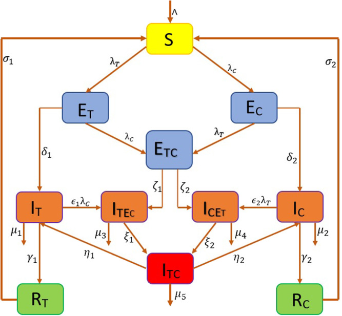
In this research study we form an epidemiological model comprising of 11 compartments, considering co-infection of two diseases namely COVID-19 and Tuberculosis. The compartments are Susceptible ($S$), population exposed to TB only ($E_T$), population exposed to COVID-19 only ($E_C$), population exposed to both TB and COVID-19 ($E_{TC}$), only TB infected individuals ($I_T$), only COVID-19 infected individuals ($I_C$), population infected with TB and exposed to COVID-19 ($I_{T{E}_C}$), population infected with COVID-19 and exposed to TB ($I_{C{E}_T}$), population infected with both COVID-19 and TB ($I_{TC}$), population recovered from TB ($R_T$), and population recovered from COVID-19 ($R_C$). The parameters involved in the model have unit as ${\text{day}}^{-1}$. We consider natural birth and death in this model and based on the below assumptions we obtain the model:

• 1.The transmission of disease occurs when the susceptible comes in contact with infected individuals, be it COVID-19 infected, TB infected or both. We assume that with the rising COVID-19 cases and TB in the corner, the susceptible population tends to wear face mask, thereby contributing in reducing the infection rates. These forces of infections are given by ${\lambda }_T$ and ${\lambda }_C$ due to TB and COVID-19 respectively, in which the face mask factor is represented by parameters ${\alpha }_1$ and ${\alpha }_2$.
• 2.It is possible that the individuals exposed to TB ($E_T$) only and COVID-19 only ($E_C$) come in contact with COVID-19 infected population and TB infected population respectively, thereby getting exposed to both these diseases.
• 3.The exposed population ($E_T$), and ($E_C$) move to their respective infected classes ($I_T$), and ($I_C$) at rates ${\delta }_1$, and ${\delta }_2$ respectively.
• 4.Since both diseases have different incubation period, an individual exposed to both COVID-19 and TB ($E_{TC}$) being infectious of both diseases at same time is unlikely. Hence, we assume that these exposed individuals move to classes $I_{T{E}_C}$ and $I_{C{E}_T}$ at rate ${\zeta }_1$ and ${\zeta }_2$ respectively. The individuals in $I_{T{E}_C}$ and $I_{C{E}_T}$ classes move to the $I_{TC}$ class at rates ${\xi }_1$ and ${\xi }_2$ respectively.
• 5.We assume that the individuals infected with TB only can come in contact with COVID-19 infected individuals, and become exposed to the latter. In this case we assume that an enhancement factor which will act as a modification parameter in transmission of infection, would contribute in increasing the infection rate, thereby the force of infection. This parameter is given by ${\epsilon }_1$ of which the value is greater than or equal to 1. The same applies to the COVID-19 only infected individuals, in which case the modification parameter is given by ${\epsilon }_2$.
• 6.Since, both these diseases have different infectious periods, the possibility of an individual recovering from both the infections at once is neglected. Hence, an individual with this co-infection can recover from one infection at a time and move to the infected class belonging to another disease at certain rates. These rates are given by ${\eta }_1$ and ${\eta }_2$.
• 7.The TB only and COVID-19 only infected individuals move to their respective recovered class at rates ${\gamma }_1$ and ${\gamma }_2$ respectively.
• 8.Having recovered from these diseases does not guarantee lifelong immunity, hence the immunity wanes, and the recovered individuals move to the susceptible class at rates ${\sigma }_1$ and ${\sigma }_2$.
• 9.The infected population die at respective disease induced death rates.

The schematic diagram of our proposed model is depicted in Fig. 1.

Fig. 1.

Schematic diagram of the model.

The model is framed into the following system of equations:

$$\frac{dS}{dt}=\wedge +{\sigma }_1{R}_T+{\sigma }_2{R}_C-({\lambda }_T+{\lambda }_C+\mu )S$$ (1)

$$\frac{d{E}_T}{dt}={\lambda }_{T}S-({\delta }_1+{\lambda }_C+\mu )E_T$$ (2)

$$\frac{d{E}_C}{dt}={\lambda }_{C}S-({\delta }_2+{\lambda }_T+\mu )E_C$$ (3)

$$\frac{d{E}_{TC}}{dt}={\lambda }_C{E}_T+{\lambda }_T{E}_C-({\zeta }_1+{\zeta }_2+\mu )E_{TC}$$ (4)

$$\frac{d{I}_T}{dt}={\delta }_1{E}_T+{\eta }_1{I}_{TC}-({\gamma }_1+{\epsilon }_1{\lambda }_C+{\mu }_1+\mu )I_T$$ (5)

$$\frac{d{I}_C}{dt}={\delta }_2{E}_C+{\eta }_2{I}_{TC}-({\gamma }_2+{\epsilon }_2{\lambda }_T+{\mu }_2+\mu )I_C$$ (6)

$$\frac{d{I}_{T{E}_C}}{dt}={\epsilon }_1{\lambda }_C{I}_T+{\zeta }_1{E}_{TC}-({\xi }_1+{\mu }_3+\mu )I_{T{E}_C}$$ (7)

$$\frac{d{I}_{C{E}_T}}{dt}={\epsilon }_2{\lambda }_T{I}_C+{\zeta }_2{E}_{TC}-({\xi }_2+{\mu }_4+\mu )I_{C{E}_T}$$ (8)

$$\frac{d{I}_{TC}}{dt}={\xi }_1{I}_{T{E}_C}+{\xi }_2{I}_{C{E}_T}-({\eta }_1+{\eta }_2++{\mu }_5+\mu )I_{TC}$$ (9)

$$\frac{d{R}_T}{dt}={\gamma }_1{I}_T-({\sigma }_1+\mu )R_T$$ (10)

$$\frac{d{R}_C}{dt}={\gamma }_2{I}_C-({\sigma }_2+\mu )R_C,$$ (11)

where

$${\lambda }_T={\beta }_1(1-{\alpha }_1)(I_T+I_{TC}+I_{T{E}_C})\text{and}{\lambda }_C={\beta }_2(1-{\alpha }_2)(I_C+I_{TC}+I_{C{E}_T})$$

3. Analysis of the model

3.1. TB only sub-model

The TB model is obtained by setting the following variables $E_C=E_{TC}=I_C=I_{T{E}_C}=I_{C{E}_T}=I_{TC}=R_C=0$.

$$\begin{array}{cc}\hfill \frac{dS}{dt}& =\wedge +{\sigma }_1{R}_T-{\beta }_1(1-{\alpha }_1)I_{T}S-\mu S\hfill \\ \hfill & \hfill \\ \hfill \frac{d{E}_T}{dt}& ={\beta }_1(1-{\alpha }_1)I_{T}S-({\delta }_1+\mu )E_T\hfill \\ \hfill & \hfill \\ \hfill \frac{d{I}_T}{dt}& ={\delta }_1{E}_T-({\gamma }_1+{\mu }_1+\mu )I_T\hfill \\ \hfill & \hfill \\ \hfill \frac{d{R}_T}{dt}& ={\gamma }_1{I}_T-({\sigma }_1+\mu )R_T\hfill \end{array}$$ (12)

The total population from the model (12) is $N=S+E_T+I_T+R_T$ and hence we have $\frac{dN}{dt}=\wedge -\mu N-{\mu }_1{I}_T$. Solving this we get ${lim\; sup}_{t\to \infty }N\le \frac{\wedge }{\mu }$, which further implies the solution of model (12) is bounded by $\frac{\wedge }{\mu }$. Therefore, biologically feasible region for the system (12) is given by: ${\Omega }_T=\left\{(S,E_T,I_T,R_T)\in {\mathbb{R}}_{+}^4:0\le S,E_T,I_T,R_T\le \frac{\wedge }{\mu }\right\}$.

3.1.1. Equilibria and basic reproduction number

The disease-free equilibrium (DFE) of the system (12) is given by $E^{0t}=\left(\frac{\wedge }{\mu },0,0,0\right)$. Using Next Generation Matrix Method [20], [25], [49] we find the basic reproduction number $R_{0_T}$.

$$\mathcal{F}=\left(\begin{array}{c}\hfill {\beta }_1(1-{\alpha }_1)I_{T}S\hfill \\ \hfill 0\hfill \end{array}\right)\mathcal{V}=\left(\begin{array}{c}\hfill ({\delta }_1+\mu )E_T\hfill \\ \hfill -{\delta }_1{E}_T+({\gamma }_1+{\mu }_1+\mu )I_T\hfill \end{array}\right)$$

The Jacobian of $\mathcal{F}$ (representing new infection terms) and $\mathcal{V}$ (representing transition terms) are F and V respectively.

$$F=\left(\begin{array}{cc}\hfill 0\hfill & \hfill {\beta }_1(1-{\alpha }_1)\frac{\wedge }{\mu }\hfill \\ \hfill 0\hfill & \hfill 0\hfill \end{array}\right)V=\left(\begin{array}{cc}\hfill {\delta }_1+\mu \hfill & \hfill 0\hfill \\ \hfill -{\delta }_1\hfill & \hfill {\gamma }_1+{\mu }_1+\mu \hfill \end{array}\right).$$

We then obtain

$$F{V}^{-1}=\left(\begin{array}{cc}\hfill \frac{{\beta }_1(1-{\alpha }_1){\delta }_1\wedge }{({\delta }_1+\mu )({\gamma }_1+{\mu }_1+\mu )\mu }\hfill & \hfill \frac{{\beta }_1(1-{\alpha }_1)\wedge }{({\gamma }_1+{\mu }_1+\mu )\mu }\hfill \\ \hfill 0\hfill & \hfill 0\hfill \end{array}\right)$$

from which we obtain the basic reproduction number which is the spectral radius of $F{V}^{-1}$, given by

$$R_{0_T}=\frac{{\beta }_1(1-{\alpha }_1){\delta }_1\wedge }{({\delta }_1+\mu )({\gamma }_1+{\mu }_1+\mu )\mu }$$

Theorem 3.1

The disease-free Equilibrium given by $E^{0t}$ is locally asymptotically stable when $R_{0_T}<1$ and is unstable otherwise.

Proof

The Jacobian matrix $J_{E^{0t}}$ of the system (12) at the disease-free equilibrium point $E^{0t}$ is obtained as below:

$$J_{E^{0t}}=\left(\begin{array}{cccc}\hfill -\mu \hfill & \hfill 0\hfill & \hfill -{\beta }_1(1-{\alpha }_1)\frac{\wedge }{\mu }\hfill & \hfill {\sigma }_1\hfill \\ \hfill 0\hfill & \hfill -({\delta }_1+\mu )\hfill & \hfill {\beta }_1(1-{\alpha }_1)\frac{\wedge }{\mu }\hfill & \hfill 0\hfill \\ \hfill 0\hfill & \hfill {\delta }_1\hfill & \hfill -({\gamma }_1+{\mu }_1+\mu )\hfill & \hfill 0\hfill \\ \hfill 0\hfill & \hfill 0\hfill & \hfill {\gamma }_1\hfill & \hfill -({\sigma }_1+\mu )\hfill \end{array}\right)$$

The characteristic polynomial $|J_{E^{0t}}-\lambda I|=0$ is given by:

$$(\lambda +\mu )\times (\lambda +({\sigma }_1+\mu ))\times \left({\lambda }^2+(({\delta }_1+\mu )+({\gamma }_1+{\mu }_1+\mu ))\lambda +({\delta }_1+\mu )({\gamma }_1+{\mu }_1+\mu )-{\beta }_1(1-{\alpha }_1){\delta }_1\frac{\wedge }{\mu }\right)=0$$

Therefore, the eigenvalues are $-\mu <0,-({\sigma }_1+\mu )<0$, and remaining are the roots of the following

$$\left({\lambda }^2+(({\delta }_1+\mu )+({\gamma }_1+{\mu }_1+\mu ))\lambda +({\delta }_1+\mu )({\gamma }_1+{\mu }_1+\mu )-{\beta }_1(1-{\alpha }_1){\delta }_1\frac{\wedge }{\mu }\right)=0.$$

Hence, the two roots are:

$$-\frac{1}{2}(({\delta }_1+\mu )+({\gamma }_1+{\mu }_1+\mu ))\pm \frac{1}{2}\sqrt{{(({\delta }_1+\mu )+({\gamma }_1+{\mu }_1+\mu ))}^2-4\left(({\delta }_1+\mu )({\gamma }_1+{\mu }_1+\mu )-{\beta }_1(1-{\alpha }_1){\delta }_1\frac{\wedge }{\mu }\right)}$$

which are both negative or have negative real part when $R_{0_T}<1$ since,

$$R_{0_T}<1⟹({\delta }_1+\mu )({\gamma }_1+{\mu }_1+\mu )-{\beta }_1(1-{\alpha }_1){\delta }_1\frac{\wedge }{\mu }>0.$$

Therefore, the disease-free equilibrium is locally asymptotically stable when $R_{0_T}<1$.

The endemic equilibrium $E^{\ast }=(S^{\ast },E_T^{\ast },I_T^{\ast },R_T^{\ast })$ of the system (12) is obtained to be as follows:

$$S^{\ast }=\frac{\left({\delta }_1\right)({\gamma }_1+{\mu }_1+\mu )}{{\beta }_1{\delta }_1(1-{\alpha }_1)},I_T^{\ast }=\frac{({\sigma }_1+\mu )({\delta }_1+\mu )({\gamma }_1+{\mu }_1+\mu )(R_{0_T}-1)}{{\beta }_1(1-{\alpha }_1)(({\delta }_1+\mu )({\gamma }_1+{\mu }_1+\mu )({\sigma }_1+\mu )-{\sigma }_1{\gamma }_1{\delta }_1)},$$

$$E_T^{\ast }=\frac{({\gamma }_1+{\mu }_1+\mu )}{{\delta }_1}{I}_T^{\ast },\text{and}{R}_T^{\ast }=\frac{{\gamma }_1}{({\sigma }_1+\mu )}{I}_T^{\ast }.$$

Clearly, the endemic equilibrium exists and is positive when $R_{0_T}>1$ and is unique for the TB only model.

3.1.2. Bifurcation and stability analysis of the endemic equilibrium

Let us denote $S=x_1,E_T=x_2,I_T=x_3,R_T=x_4$, so that the TB only model (12) can be written as follows:

$$\begin{array}{cc}\hfill \frac{d{x}_1}{dt}& =f_1=\wedge +{\sigma }_1{x}_4-{\beta }_1(1-{\alpha }_1)x_3{x}_1-\mu x_1\hfill \\ \hfill & \hfill \\ \hfill \frac{d{x}_2}{dt}& =f_2={\beta }_1(1-{\alpha }_1)x_3{x}_1-({\delta }_1+\mu )x_2\hfill \\ \hfill & \hfill \\ \hfill \frac{d{x}_3}{dt}& =f_3={\delta }_1{x}_2-({\gamma }_1+{\mu }_1+\mu )x_3\hfill \\ \hfill & \hfill \\ \hfill \frac{d{x}_4}{dt}& =f_4={\gamma }_1{x}_3-({\sigma }_1+\mu )x_4\hfill \end{array}$$ (13)

The Jacobian of the above system (13) at the DFE $E^{0t}$ at the chosen bifurcation parameter ${\beta }_1$, obtained by equating $R_{0_T}=1$ is

$$J_{E^{0t}({\beta }_1={\beta }_1^{\ast })}=\left(\begin{array}{cccc}\hfill -\mu \hfill & \hfill 0\hfill & \hfill -\frac{({\delta }_1+\mu )({\gamma }_1+{\mu }_1+\mu )}{{\delta }_1}\hfill & \hfill {\sigma }_1\hfill \\ \hfill 0\hfill & \hfill -({\delta }_1+\mu )\hfill & \hfill \frac{({\delta }_1+\mu )({\gamma }_1+{\mu }_1+\mu )}{{\delta }_1}\hfill & \hfill 0\hfill \\ \hfill 0\hfill & \hfill {\delta }_1\hfill & \hfill -({\gamma }_1+{\mu }_1+\mu )\hfill & \hfill 0\hfill \\ \hfill 0\hfill & \hfill 0\hfill & \hfill {\gamma }_1\hfill & \hfill -({\sigma }_1+\mu )\hfill \end{array}\right)$$

Here, ${\beta }_1^{\ast }=\frac{({\delta }_1+\mu )({\gamma }_1+{\mu }_1+\mu )\mu }{(1-{\alpha }_1)\wedge {\delta }_1}$ obtained by equating $R_{0_T}=1$. The above linearized system with ${\beta }_1={\beta }_1^{\ast }$ has a zero eigenvalue. We therefore use centre manifold theory [12], [13] to analyse the dynamics of the system near ${\beta }_1={\beta }_1^{\ast }$. We use the theorem in [13], which we have stated in the Appendix section as Theorem A.1, to show the stability of TB only endemic equilibrium point ($E^{\ast }$). We now obtain the left and the right eigenvectors associated to the zero eigenvalue of the Jacobian, $J_{E^{0t}({\beta }_1={\beta }_1^{\ast })}$.

Using the same notation as in Theorem A.1, we denote the right eigenvector (the column matrix) as $w={[w_1,w_2,w_3,w_4]}^T$, where

$$w_1=\frac{-(({\delta }_1+\mu )({\gamma }_1+{\mu }_1+\mu )({\sigma }_1+\mu )-{\sigma }_1{\gamma }_1{\delta }_1)w_4}{\mu {\gamma }_1{\delta }_1},w_2=\frac{({\gamma }_1+{\mu }_1+\mu )({\sigma }_1+\mu )w_4}{{\delta }_1{\gamma }_1}$$

$$w_3=\frac{({\sigma }_1+\mu )w_4}{{\gamma }_1},\text{and}{w}_4=w_4>0,$$

and the left eigenvector (the row matrix) associated with the zero eigenvalue as $v=[v_1,v_2,v_3,v_4]$, where $v_1=0=v_4,v_2=\frac{{\delta }_1}{{\delta }_1+\mu }{v}_3,\text{and}{v}_3=v_3>0$. Continuing as per the theorem, we now compute $a$ and $b$ to do the bifurcation analysis by finding the non-zero partial derivatives associated with the system (13) at the disease-free equilibrium point ($E^{0t}$). These partial derivatives are:

$$\frac{{\partial }^2{f}_2}{\partial x_1\partial x_3}={\beta }_1^{\ast }(1-{\alpha }_1)=\frac{({\delta }_1+\mu )({\gamma }_1+{\mu }_1+\mu )\mu }{\wedge {\delta }_1}=\frac{{\partial }^2{f}_2}{\partial x_3\partial x_1},\frac{{\partial }^2{f}_2}{\partial x_3\partial {\beta }_1}=(1-{\alpha }_1)\frac{\wedge }{\mu }\therefore a=-\frac{2v_3{w}_4^2(({\gamma }_1+{\mu }_1+\mu )({\delta }_1+\mu )({\sigma }_1+\mu )-{\gamma }_1{\delta }_1{\sigma }_1)({\gamma }_1+{\mu }_1+\mu )({\sigma }_1+\mu )}{\wedge {\delta }_1{\gamma }_1^2}<0$$

$$\text{and}b=\frac{{\delta }_1\wedge v_3{w}_4(1-{\alpha }_1)({\sigma }_1+\mu )}{\mu {\gamma }_1({\delta }_1+\mu )}>0.$$

Since $a<0$ and $b>0$, from the theorem in [13] (Theorem A.1), it implies that the unique TB only endemic equilibrium point ($E^{\ast }$) which exists when $R_{0_T}>1$ will be locally asymptotically stable and the system will not exhibit any backward bifurcation at $R_{0_T}=1$. Therefore we have the following theorem established.

Theorem 3.2

The unique endemic equilibrium ( $E^{\ast }$ ) of the system (12) is locally asymptotically stable when $R_{0_T}>1$ .

3.2. COVID-19 only sub-model

The COVID-19 model is obtained by setting the following variables $E_T=E_{TC}=I_T=I_{T{E}_C}=I_{C{E}_T}=I_{TC}=R_T=0$.

$$\begin{array}{cc}\hfill \frac{dS}{dt}& =\wedge +{\sigma }_2{R}_C-{\beta }_2(1-{\alpha }_2)I_{C}S-\mu S\hfill \\ \hfill & \hfill \\ \hfill \frac{d{E}_C}{dt}& ={\beta }_2(1-{\alpha }_2)I_{C}S-({\delta }_2+\mu )E_C\hfill \\ \hfill & \hfill \\ \hfill \frac{d{I}_C}{dt}& ={\delta }_2{E}_C-({\gamma }_2+{\mu }_2+\mu )I_C\hfill \\ \hfill & \hfill \\ \hfill \frac{d{R}_C}{dt}& ={\gamma }_2{I}_C-({\sigma }_2+\mu )R_C\hfill \end{array}$$ (14)

The total population from the model (14) is $N=S+E_C+I_C+R_C$ and hence we have $\frac{dN}{dt}=\wedge -\mu N-{\mu }_2{I}_C$. Solving this we get ${lim\; sup}_{t\to \infty }N\le \frac{\wedge }{\mu }$, which further implies the solution of model (14) is bounded by $\frac{\wedge }{\mu }$. Therefore, biologically feasible region for the system (14) is given by: ${\Omega }_C=\left\{(S,E_C,I_C,R_C)\in {\mathbb{R}}_{+}^4:0\le S,E_C,I_C,R_C\le \frac{\wedge }{\mu }\right\}$.

3.2.1. Equilibria and basic reproduction number

The disease-free equilibrium (DFE) of the system (14) is given by $E^{0c}=\left(\frac{\wedge }{\mu },0,0,0\right)$. Using Next Generation Matrix Method [20], [25], [49] we find the basic reproduction number $R_{0_C}$.

$$\mathcal{F}=\left(\begin{array}{c}\hfill {\beta }_2(1-{\alpha }_2)I_{C}S\hfill \\ \hfill 0\hfill \end{array}\right)\mathcal{V}=\left(\begin{array}{c}\hfill ({\delta }_2+\mu )E_C\hfill \\ \hfill -{\delta }_2{E}_C+({\gamma }_2+{\mu }_2+\mu )I_C\hfill \end{array}\right)$$

The Jacobian of $\mathcal{F}$ (representing new infection terms) and $\mathcal{V}$ (representing transition terms) are F and V respectively.

$$F=\left(\begin{array}{cc}\hfill 0\hfill & \hfill {\beta }_2(1-{\alpha }_2)\frac{\wedge }{\mu }\hfill \\ \hfill 0\hfill & \hfill 0\hfill \end{array}\right)V=\left(\begin{array}{cc}\hfill {\delta }_2+\mu \hfill & \hfill 0\hfill \\ \hfill -{\delta }_2\hfill & \hfill {\gamma }_2+{\mu }_2+\mu \hfill \end{array}\right)$$

We then obtain,

$$F{V}^{-1}=\left(\begin{array}{cc}\hfill \frac{{\beta }_2(1-{\alpha }_2){\delta }_2\wedge }{({\delta }_2+\mu )({\gamma }_2+{\mu }_2+\mu )\mu }\hfill & \hfill \frac{{\beta }_2(1-{\alpha }_2)\wedge }{({\gamma }_2+{\mu }_2+\mu )\mu }\hfill \\ \hfill 0\hfill & \hfill 0\hfill \end{array}\right)$$

The basic reproduction number is the spectral radius of $F{V}^{-1}$, which is given by

$$R_{0_C}=\frac{{\beta }_2(1-{\alpha }_2){\delta }_2\wedge }{({\delta }_2+\mu )({\gamma }_2+{\mu }_2+\mu )\mu }$$

Theorem 3.3

The disease-free Equilibrium given by $E^{0c}$ is locally asymptotically stable when $R_{0_C}<1$ and is unstable otherwise.

Proof

The Jacobian matrix $J_{E^{0c}}$ of the system (14) at the disease-free equilibrium point $E^{0c}$ is obtained as below:

$$J_{E^{0c}}=\left(\begin{array}{cccc}\hfill -\mu \hfill & \hfill 0\hfill & \hfill -{\beta }_2(1-{\alpha }_2)\frac{\wedge }{\mu }\hfill & \hfill {\sigma }_2\hfill \\ \hfill 0\hfill & \hfill -({\delta }_2+\mu )\hfill & \hfill {\beta }_2(1-{\alpha }_2)\frac{\wedge }{\mu }\hfill & \hfill 0\hfill \\ \hfill 0\hfill & \hfill {\delta }_2\hfill & \hfill -({\gamma }_2+{\mu }_2+\mu )\hfill & \hfill 0\hfill \\ \hfill 0\hfill & \hfill 0\hfill & \hfill {\gamma }_2\hfill & \hfill -({\sigma }_2+\mu )\hfill \end{array}\right)$$

The characteristic polynomial $|J_{E^{0c}}-\lambda I|=0$ is given by:

$$(\lambda +\mu )\times (\lambda +({\sigma }_2+\mu ))\times \left({\lambda }^2+(({\delta }_2+\mu )+({\gamma }_2+{\mu }_2+\mu ))\lambda +({\delta }_2+\mu )({\gamma }_2+{\mu }_2+\mu )-{\beta }_2(1-{\alpha }_2){\delta }_2\frac{\wedge }{\mu }\right)=0$$

Therefore, the eigenvalues are $-\mu <0,-({\sigma }_2+\mu )<0$, and remaining are the roots of the following

$$\left({\lambda }^2+(({\delta }_2+\mu )+({\gamma }_2+{\mu }_2+\mu ))\lambda +({\delta }_2+\mu )({\gamma }_2+{\mu }_2+\mu )-{\beta }_2(1-{\alpha }_2){\delta }_2\frac{\wedge }{\mu }\right)=0.$$

Hence the two roots are:

$$-\frac{1}{2}(({\delta }_2+\mu )+({\gamma }_2+{\mu }_2+\mu ))\pm \frac{1}{2}\sqrt{{(({\delta }_2+\mu )+({\gamma }_2+{\mu }_2+\mu ))}^2-4\left(({\delta }_2+\mu )({\gamma }_2+{\mu }_2+\mu )-{\beta }_2(1-{\alpha }_2){\delta }_2\frac{\wedge }{\mu }\right)}$$

which are both negative or have negative real part when $R_{0_C}<1$ since,

$$R_{0_C}<1⟹({\delta }_2+\mu )({\gamma }_2+{\mu }_2+\mu )-{\beta }_2(1-{\alpha }_2){\delta }_2\frac{\wedge }{\mu }>0$$

Therefore, the disease-free equilibrium is locally asymptotically stable when $R_{0_C}<1$.

The endemic equilibrium $E^{\star }=(S^{\star },E_C^{\star },I_C^{\star },R_C^{\star })$ of the system (14) is obtained to be as follows: 

$$S^{\star }=\frac{\left({\delta }_2\right)({\gamma }_2+{\mu }_2+\mu )}{{\beta }_2{\delta }_2(1-{\alpha }_2)},I_C^{\star }=\frac{({\sigma }_2+\mu )({\delta }_2+\mu )({\gamma }_2+{\mu }_2+\mu )(R_{0_C}-1)}{{\beta }_2(1-{\alpha }_2)(({\delta }_2+\mu )({\gamma }_2+{\mu }_2+\mu )({\sigma }_2+\mu )-{\sigma }_2{\gamma }_2{\delta }_2)},$$

$$E_C^{\star }=\frac{({\gamma }_2+{\mu }_2+\mu )}{{\delta }_2}{I}_C^{\star },\text{and}{R}_C^{\star }=\frac{{\gamma }_2}{({\sigma }_2+\mu )}{I}_C^{\star }.$$

Clearly, the COVID-19 only endemic equilibrium ($E^{\star }$) exists when $R_{0_C}>1$ and is unique for the COVID-19 only model (14).

3.2.2. Bifurcation and stability analysis of the endemic equilibrium

Let us denote $S=x_1,E_C=x_2,I_C=x_3,R_C=x_4$, so that the COVID-19 only model can be written as follows:

$$\begin{array}{cc}\hfill \frac{d{x}_1}{dt}& =f_1=\wedge +{\sigma }_2{x}_4-{\beta }_2(1-{\alpha }_2)x_3{x}_1-\mu x_1\hfill \\ \hfill & \hfill \\ \hfill \frac{d{x}_2}{dt}& =f_2={\beta }_2(1-{\alpha }_2)x_3{x}_1-({\delta }_2+\mu )x_2\hfill \\ \hfill & \hfill \\ \hfill \frac{d{x}_3}{dt}& =f_3={\delta }_2{x}_2-({\gamma }_2+{\mu }_2+\mu )x_3\hfill \\ \hfill & \hfill \\ \hfill \frac{d{x}_4}{dt}& =f_4={\gamma }_2{x}_3-({\sigma }_2+\mu )x_4\hfill \end{array}$$ (15)

The Jacobian of the system (15) at the DFE ($E^{0c}$) at the chosen bifurcation parameter ${\beta }_2$, obtained by equating $R_{0_C}=1$ is

$$J_{E^{0c}({\beta }_2={\beta }_2^{\ast })}=\left(\begin{array}{cccc}\hfill -\mu \hfill & \hfill 0\hfill & \hfill -\frac{({\delta }_2+\mu )({\gamma }_2+{\mu }_2+\mu )}{{\delta }_2}\hfill & \hfill {\sigma }_2\hfill \\ \hfill 0\hfill & \hfill -({\delta }_2+\mu )\hfill & \hfill \frac{({\delta }_2+\mu )({\gamma }_2+{\mu }_2+\mu )}{{\delta }_2}\hfill & \hfill 0\hfill \\ \hfill 0\hfill & \hfill {\delta }_2\hfill & \hfill -({\gamma }_2+{\mu }_2+\mu )\hfill & \hfill 0\hfill \\ \hfill 0\hfill & \hfill 0\hfill & \hfill {\gamma }_2\hfill & \hfill -({\sigma }_2+\mu )\hfill \end{array}\right)$$

Here, ${\beta }_2^{\ast }=\frac{({\delta }_2+\mu )({\gamma }_2+{\mu }_2+\mu )\mu }{(1-{\alpha }_2)\wedge {\delta }_2}$ obtained by equating $R_{0_C}=1$. The above linearized system with ${\beta }_2={\beta }_2^{\ast }$ has zero eigenvalue. We therefore use centre manifold theory [12], [13] to analyse the dynamics of the system near ${\beta }_2={\beta }_2^{\ast }$. We use the theorem in [13], which we have stated in the Appendix section as Theorem A.1, to show the stability of COVID-19 only endemic equilibrium point ($E^{\star }$). We now obtain the left and the right eigenvectors associated to the zero eigenvalue of the Jacobian $J_{E^{0c}({\beta }_2={\beta }_2^{\ast })}$. Using the same notation as in Theorem A.1, we denote the right eigenvector (the column matrix) as $w={[w_1,w_2,w_3,w_4]}^T$, where

$$w_1=\frac{-(({\delta }_2+\mu )({\gamma }_2+{\mu }_2+\mu )({\sigma }_2+\mu )-{\sigma }_2{\gamma }_2{\delta }_2)w_4}{\mu {\gamma }_2{\delta }_2},w_2=\frac{({\gamma }_2+{\mu }_2+\mu )({\sigma }_2+\mu )w_4}{{\delta }_2{\gamma }_2}$$

$$w_3=\frac{({\sigma }_2+\mu )w_4}{{\gamma }_2},\text{and}{w}_4=w_4>0,$$

and the left eigenvector (the row matrix) associated with the zero eigenvalue as $v=[v_1,v_2,v_3,v_4]$, where $v_1=0=v_4,v_2=\frac{{\delta }_2}{{\delta }_2+\mu }{v}_3,\text{and}{v}_3=v_3>0$.

Continuing as per the theorem, we now compute $a$ and $b$ to do the bifurcation analysis by finding the non-zero partial derivatives associated with the system (15) at the disease-free equilibrium point ($E^{0c}$). These partial derivatives are:

$$\frac{{\partial }^2{f}_2}{\partial x_1\partial x_3}={\beta }_2^{\ast }(1-{\alpha }_2)=\frac{({\delta }_2+\mu )({\gamma }_2+{\mu }_2+\mu )\mu }{\wedge {\delta }_2}=\frac{{\partial }^2{f}_2}{\partial x_3\partial x_1},\frac{{\partial }^2{f}_2}{\partial x_3\partial {\beta }_2}=(1-{\alpha }_2)\frac{\wedge }{\mu }.\therefore a=-\frac{2v_3{w}_4^2(({\gamma }_2+{\mu }_2+\mu )({\delta }_2+\mu )({\sigma }_2+\mu )-{\gamma }_2{\delta }_2{\sigma }_2)({\gamma }_2+{\mu }_2+\mu )({\sigma }_2+\mu )}{\wedge {\delta }_2{\gamma }_2^2}<0$$

$$\text{and}b=\frac{{\delta }_2\wedge v_3{w}_4(1-{\alpha }_2)({\sigma }_2+\mu )}{\mu {\gamma }_2({\delta }_2+\mu )}>0.$$

Since $a<0$ and $b>0$, from the theorem in [13] (Theorem A.1), it implies that the unique COVID-19 only endemic equilibrium point ($E^{\star }$) which exists when $R_{0_C}>1$ will be locally asymptotically stable and the system will not exhibit any backward bifurcation at $R_{0_C}=1$. Therefore we have the following theorem established.

Theorem 3.4

The unique endemic equilibrium ( $E^{\star }$ ) of the system (14) is locally asymptotically stable when $R_{0_C}>1$ .

3.3. TB - COVID-19 complete model

The TB - COVID-19 complete model is given by the system of Eqs. (1)–(11). The total population from the model (1)–(11) is $N=S+E_T+E_C+E_{TC}+I_T+I_C+I_{T{E}_C}+I_{C{E}_T}+I_{TC}+R_T+R_C$ and hence we have $\frac{dN}{dt}=\wedge -\mu N-{\mu }_1{I}_T-{\mu }_2{I}_C-{\mu }_3{I}_{T{E}_C}-{\mu }_4{I}_{C{E}_T}-{\mu }_5{I}_{TC}$. Solving this we get ${lim\; sup}_{t\to \infty }N\le \frac{\wedge }{\mu }$, which further implies the solution of model (1)–(11) is bounded by $\frac{\wedge }{\mu }$. Therefore, biologically feasible region for the system (1)–(11) is given by:

$${\Omega }_{TC}=\left\{(S,E_T,E_C,E_{TC},I_T,I_C,I_{T{E}_C},I_{C{E}_T},I_{TC},R_T,R_C)\in {\mathbb{R}}_{+}^{11}\right)\left(:0\le S,E_T,E_C,E_{TC},I_T,I_C,I_{T{E}_C},I_{C{E}_T},I_{TC},R_T,R_C\le \frac{\wedge }{\mu }\right\}.$$

Lemma 3.5

If $S\left(0\right)\ge 0,E_T\left(0\right)\ge 0,E_C\left(0\right)\ge 0,E_{TC}\left(0\right)\ge 0,I_T\left(0\right)\ge 0,I_C\left(0\right)\ge 0,I_{T{E}_C}\left(0\right)\ge 0,I_{C{E}_T}\left(0\right)\ge 0,I_{TC}\left(0\right)\ge 0,R_T\left(0\right)\ge 0,\text{and}{R}_C\left(0\right)\ge 0$ , then the solutions $S,E_T,E_C,E_{TC},I_T,I_C$ , $I_{T{E}_C},I_{C{E}_T},I_{TC},R_T,R_C$ are positive $\forall t>0$ .

Proof

We prove this lemma by method of contradiction by assuming that the total population $N\left(t\right)\ne 0\forall t\ge 0$. We assume that $\exists$ a first time $t_1$ such that:

$$S\left(t_1\right)=0,S^{\prime }\left(t_1\right)<0,E_T\left(t\right)\ge 0,E_C\left(t\right)\ge 0,E_{TC}\left(t\right)\ge 0,I_T\left(t\right)\ge 0,I_C\left(t\right)\ge 0,I_{T{E}_C}\left(t\right)\ge 0,I_{C{E}_T}\left(t\right)\ge 0,I_{TC}\left(t\right)\ge 0,R_T\left(t\right)\ge 0,\text{and}{R}_C\left(t\right)\ge 0\text{ for }t\le 0\le t_1,$$

$$\exists \text{a first time}{t}_2\text{such that}:E_T\left(t_2\right)=0,E_T^{\prime }\left(t_2\right)<0,S\left(t\right)\ge 0,E_C\left(t\right)\ge 0,E_{TC}\left(t\right)\ge 0,I_T\left(t\right)\ge 0,I_C\left(t\right)\ge 0,I_{T{E}_C}\left(t\right)\ge 0,I_{C{E}_T}\left(t\right)\ge 0,I_{TC}\left(t\right)\ge 0,R_T\left(t\right)\ge 0,\text{and}{R}_C\left(t\right)\ge 0\text{ for }t\le 0\le t_2,$$

$$\exists \text{a first time}{t}_3\text{such that}:E_C\left(t_3\right)=0,E_C^{\prime }\left(t_3\right)<0,S\left(t\right)\ge 0,E_T\left(t\right)\ge 0,E_{TC}\left(t\right)\ge 0,I_T\left(t\right)\ge 0,I_C\left(t\right)\ge 0,I_{T{E}_C}\left(t\right)\ge 0,I_{C{E}_T}\left(t\right)\ge 0,I_{TC}\left(t\right)\ge 0,R_T\left(t\right)\ge 0,\text{and}{R}_C\left(t\right)\ge 0\text{ for }t\le 0\le t_3,\exists \text{a first time}{t}_4\text{such that}:E_{TC}\left(t_4\right)=0,E_{TC}^{\prime }\left(t_4\right)<0,S\left(t\right)\ge 0,E_T\left(t\right)\ge 0,E_C\left(t\right)\ge 0,I_T\left(t\right)\ge 0,I_C\left(t\right)\ge 0,I_{T{E}_C}\left(t\right)\ge 0,I_{C{E}_T}\left(t\right)\ge 0,I_{TC}\left(t\right)\ge 0,R_T\left(t\right)\ge 0,and{R}_C\left(t\right)\ge 0\text{ for }t\le 0\le t_4,\exists \text{a first time}{t}_5\text{such that}:I_T\left(t_5\right)=0,I_T^{\prime }\left(t_5\right)<0,S\left(t\right)\ge 0,E_T\left(t\right)\ge 0,E_C\left(t\right)\ge 0,E_{TC}\left(t\right)\ge 0,I_C\left(t\right)\ge 0,I_{T{E}_C}\left(t\right)\ge 0,I_{C{E}_T}\left(t\right)\ge 0,I_{TC}\left(t\right)\ge 0,R_T\left(t\right)\ge 0,\text{and}{R}_C\left(t\right)\ge 0\text{ for }t\le 0\le t_5,\exists \text{a first time}{t}_6\text{such that}:I_C\left(t_6\right)=0,I_C^{\prime }\left(t_6\right)<0,S\left(t\right)\ge 0,E_T\left(t\right)\ge 0,E_C\left(t\right)\ge 0,E_{TC}\left(t\right)\ge 0,I_T\left(t\right)\ge 0,I_{T{E}_C}\left(t\right)\ge 0,I_{C{E}_T}\left(t\right)\ge 0,I_{TC}\left(t\right)\ge 0,R_T\left(t\right)\ge 0,\text{and}{R}_C\left(t\right)\ge 0\text{ for }t\le 0\le t_6,\exists \text{a first time}{t}_7\text{such that}:I_{T{E}_C}\left(t_7\right)=0,I_{T{E}_C}^{\prime }\left(t_7\right)<0,S\left(t\right)\ge 0,E_T\left(t\right)\ge 0,E_C\left(t\right)\ge 0,E_{TC}\left(t\right)\ge 0,I_T\left(t\right)\ge 0,I_C\left(t\right)\ge 0,I_{C{E}_T}\left(t\right)\ge 0,I_{TC}\left(t\right)\ge 0,R_T\left(t\right)\ge 0,\text{and}{R}_C\left(t\right)\ge 0\text{ for }t\le 0\le t_7,\exists \text{a first time}{t}_8\text{such that}:I_{C{E}_T}\left(t_8\right)=0,I_{C{E}_T}^{\prime }\left(t_8\right)<0,S\left(t\right)\ge 0,E_T\left(t\right)\ge 0,E_C\left(t\right)\ge 0,E_{TC}\left(t\right)\ge 0,I_T\left(t\right)\ge 0,I_C\left(t\right)\ge 0,I_{T{E}_C}\left(t\right)\ge 0,I_{TC}\left(t\right)\ge 0,R_T\left(t\right)\ge 0,\text{and}{R}_C\left(t\right)\ge 0\text{ for }t\le 0\le t_8,\exists \text{a first time}{t}_9\text{such that}:I_{TC}\left(t_9\right)=0,I_{TC}^{\prime }\left(t_9\right)<0,S\left(t\right)\ge 0,E_T\left(t\right)\ge 0,E_C\left(t\right)\ge 0,E_{TC}\left(t\right)\ge 0,I_T\left(t\right)\ge 0,I_C\left(t\right)\ge 0,I_{T{E}_C}\left(t\right)\ge 0,I_{C{E}_T}\left(t\right)\ge 0,R_T\left(t\right)\ge 0,\text{and}{R}_C\left(t\right)\ge 0\text{ for }t\le 0\le t_9,\exists \text{a first time}{t}_{10}\text{such that}:R_T\left(t_{10}\right)=0,R_T^{\prime }\left(t_{10}\right)<0,S\left(t\right)\ge 0,E_T\left(t\right)\ge 0,E_C\left(t\right)\ge 0,E_{TC}\left(t\right)\ge 0,I_T\left(t\right)\ge 0,I_C\left(t\right)\ge 0,I_{T{E}_C}\left(t\right)\ge 0,I_{C{E}_T}\left(t\right)\ge 0,I_{TC}\left(t\right)\ge 0,\text{and}{R}_C\left(t\right)\ge 0\text{ for }t\le 0\le t_{10},\exists \text{a first time}{t}_{11}\text{such that}:R_C\left(t_{11}\right)=0,R_C^{\prime }\left(t_{11}\right)<0,S\left(t\right)\ge 0,E_T\left(t\right)\ge 0,E_C\left(t\right)\ge 0,E_{TC}\left(t\right)\ge 0,I_T\left(t\right)\ge 0,I_C\left(t\right)\ge 0,I_{T{E}_C}\left(t\right)\ge 0,I_{C{E}_T}\left(t\right)\ge 0,I_{TC}\left(t\right)\ge 0,\text{and}{R}_T\left(t\right)\ge 0\text{ for }t\le 0\le t_{11}.$$

From the above equations, we verify that, $S^{\prime }\left(t_1\right)=\wedge +{\sigma }_1{R}_T\left(t_1\right)+{\sigma }_2{R}_C\left(t_1\right)>0$,

$E_T^{\prime }\left(t_2\right)={\beta }_1(1-{\alpha }_1)(I_T\left(t_2\right)+I_{TC}\left(t_2\right)+I_{T{E}_C}\left(t_2\right))S\left(t_2\right)\ge 0$ and similarly we verify that $E_C^{\prime }\left(t_3\right)\ge 0$, $E_{TC}^{\prime }\left(t_4\right)\ge 0$, $I_T^{\prime }\left(t_5\right)\ge 0$, $I_C^{\prime }\left(t_6\right)\ge 0$, $I_{T{E}_C}^{\prime }\left(t_7\right)\ge 0$, $I_{C{E}_T}^{\prime }\left(t_8\right)\ge 0$, $I_{TC}^{\prime }\left(t_9\right)\ge 0$, $R_T^{\prime }\left(t_{10}\right)\ge 0$ and $R_C^{\prime }\left(t_{11}\right)\ge 0$.

Each of these are contradicting with our assumption. Therefore, we conclude that for $t\ge 0$ we have $S\left(t\right)\ge 0,E_T\left(t\right)\ge 0,E_C\left(t\right)\ge 0,E_{TC}\left(t\right)\ge 0,I_T\left(t\right)\ge 0,I_C\left(t\right)\ge 0,I_{T{E}_C}\left(t\right)\ge 0,I_{C{E}_T}\left(t\right)\ge 0,I_{TC}\left(t\right)\ge 0,R_T\left(t\right)\ge 0,\text{and}{R}_C\left(t\right)\ge 0$. Hence, the solutions of the system (1)–(11) remain positive $\forall t\ge 0$.

3.3.1. Equilibria and basic reproduction number

The TB-COVID-19 model has 4 equilibrium points namely the disease-free equilibrium $E^0=\left(\frac{\wedge }{\mu },0,0,0,0,0,0,0,0,0,0\right)$, TB only equilibrium $E^{\ast }=(S^{\ast },E_T^{\ast },0,0,I_T^{\ast },0,0,0,0,R_T^{\ast },0)$, COVID-19 only equilibrium $E^{\star }=(S^{\star },0,E_C^{\star },0,0,I_C^{\star },0,0,0,0,R_C^{\star })$ and the endemic equilibrium (coexistence of both the disease) $E^{\ast \ast }=(S^{\ast \ast },E_T^{\ast \ast },E_C^{\ast \ast },E_{TC}^{\ast \ast },I_T^{\ast \ast },I_C^{\ast \ast },I_{T{E}_C}^{\ast \ast },I_{C{E}_T}^{\ast \ast },I_{Tc}^{\ast \ast },R_T^{\ast \ast },R_C^{\ast \ast })$. The coexistence endemic equilibrium is given by:

$$S^{\ast \ast }=\frac{\wedge +A_1{I}_T^{\ast \ast }+A_2{I}_C^{\ast \ast }}{A_3{z}_1+A_4{z}_2+\mu },E_T^{\ast \ast }=\frac{A_3{z}_1{S}^{\ast \ast }}{A_4{z}_2+({\delta }_1+\mu )},E_C^{\ast \ast }=\frac{A_4{z}_2{S}^{\ast \ast }}{A_3{z}_1+({\delta }_2+\mu )},$$

$$E_{TC}^{\ast \ast }=\frac{A_4{z}_2{E}_T^{\ast \ast }+A_3{z}_1{E}_C^{\ast \ast }}{{\zeta }_1+{\zeta }_2+\mu },I_{T{E}_C}^{\ast \ast }=\frac{{\epsilon }_1{A}_4{z}_2{I}_T^{\ast \ast }+{\zeta }_1{E}_{TC}^{\ast \ast }}{{\xi }_1+{\mu }_3+\mu },I_{C{E}_T}^{\ast \ast }=\frac{{\epsilon }_2{A}_3{z}_1{I}_C^{\ast \ast }+{\zeta }_2{E}_{TC}^{\ast \ast }}{{\xi }_2+{\mu }_4+\mu },$$

$$I_{TC}^{\ast \ast }=\frac{{\xi }_1{I}_{T{E}_C}^{\ast \ast }+{\xi }_2{I}_{C{E}_T}^{\ast \ast }}{{\eta }_1+{\eta }_2+{\mu }_5+\mu },R_T^{\ast \ast }=\frac{{\gamma }_1{T}_T^{\ast \ast }}{{\sigma }_1+\mu },R_C^{\ast \ast }=\frac{{\gamma }_2{T}_C^{\ast \ast }}{{\sigma }_2+\mu }.$$

The above expressions are in $z_1,z_2,I_T,\text{and}{I}_C$, where $z_1=I_T+I_{TC}+I_{T{E}_C}$ and $z_2=I_C+I_{TC}+I_{C{E}_T}$. This implies that these variables are in terms of $I_T,I_C,I_{T{E}_C},\text{and}{I}_{C{E}_T}$. Using these we get four equations as below, which when solved gives us $I_T^{\ast \ast },I_C^{\ast \ast },I_{T{E}_C}^{\ast \ast },I_{C{E}_T}^{\ast \ast }$ and hence we get the endemic equilibrium $E^{\ast \ast }$. These four equations are,

$$\{[A_4(I_C+C_1{I}_{T{E}_C}+(C_2+1)I_{C{E}_T})+({\delta }_1+\mu )][A_3(I_T+(C_1+1)I_{T{E}_C}+C_2{I}_{C{E}_T})+A_4(I_C+C_1{I}_{T{E}_C}+(C_2+1)I_{C{E}_T})+\mu ]\}\times [I_{T{E}_C}({\eta }_1{C}_1-{\epsilon }_1{\beta }_2(1-{\alpha }_2)C_1{I}_T)+I_{C{E}_T}({\eta }_1{C}_2-{\epsilon }_1{\beta }_2(1-{\alpha }_2)(C_2+1)I_T)-{\epsilon }_1{\beta }_2(1-{\alpha }_2)I_T{I}_C-({\gamma }_1+{\mu }_1+\mu )I_T]+{\delta }_1{A}_3[I_T+(C_1+1)I_{T{E}_C}+C_2{I}_{C{E}_T}](\wedge +A_1{I}_T+A_2{I}_C)=0$$

$$\{[A_3(I_T+(C_1+1)I_{T{E}_C}+C_2{I}_{C{E}_T})+({\delta }_2+\mu )][A_3(I_T+(C_1+1)I_{T{E}_C}+C_2{I}_{C{E}_T})+A_4(I_C+C_1{I}_{T{E}_C}+(C_2+1)I_{C{E}_T})+\mu ]\}\times [I_{T{E}_C}({\eta }_2{C}_1-{\epsilon }_2{\beta }_1(1-{\alpha }_1)(C_1+1)I_C)+I_{C{E}_T}({\eta }_2{C}_2-{\epsilon }_2{\beta }_1(1-{\alpha }_1)C_1{I}_C)-{\epsilon }_2{\beta }_1(1-{\alpha }_1)I_T{I}_C-({\gamma }_2+{\mu }_2+\mu )I_C]+{\delta }_2{A}_4[I_C+C_1{I}_{T{E}_C}+(C_2+1)I_{C{E}_T}](\wedge +A_1{I}_T+A_2{I}_C)=0$$

$$[{\epsilon }_1{\beta }_2(1-{\alpha }_2)(I_C+C_1{I}_{T{E}_C}+(C_2+1)I_{C{E}_T})I_T-({\xi }_1+{\mu }_3+\mu )I_{T{E}_C}]\times \{[A_3(I_T+(C_1+1)I_{T{E}_C}+C_2{I}_{C{E}_T})+A_4(I_C+C_1{I}_{T{E}_C}+(C_2+1)I_{C{E}_T})+\mu ]\times [A_4(I_C+C_1{I}_{T{E}_C}+(C_2+1)I_{C{E}_T})+({\delta }_1+\mu )]\times \left[A_3(I_T+(C_1+1)I_{T{E}_C}+C_2{I}_{C{E}_T})\right]\}+(\wedge +A_1{I}_T+A_2{I}_C)\{[A_3(I_T+(C_1+1)I_{T{E}_C}+C_2{I}_{C{E}_T})+({\delta }_2+\mu )]\times \left[A_3(I_T+(C_1+1)I_{T{E}_C}+C_2{I}_{C{E}_T})\right]\times \left[{\zeta }_1{G}_1(I_C+C_1{I}_{T{E}_C}+(C_2+1)I_{C{E}_T})\right]+[A_4(I_C+C_1{I}_{T{E}_C}+(C_2+1)I_{C{E}_T})+({\delta }_1+\mu )]\times \left[A_4(I_C+C_1{I}_{T{E}_C}+(C_2+1)I_{C{E}_T})\right]\times \left[{\zeta }_1{G}_2(I_T+(C_1+1)I_{T{E}_C}+C_2{I}_{C{E}_T})\right]\}=0$$

$$[{\epsilon }_2{\beta }_1(1-{\alpha }_1)(I_T+(C_1+1)I_{T{E}_C}+C_2{I}_{C{E}_T})I_C-({\xi }_2+{\mu }_4+\mu )I_{C{E}_T}]\times \{[A_3(I_T+(C_1+1)I_{T{E}_C}+C_2{I}_{C{E}_T})+A_4(I_C+C_1{I}_{T{E}_C}+(C_2+1)I_{C{E}_T})+\mu ]\times [A_4(I_C+C_1{I}_{T{E}_C}+(C_2+1)I_{C{E}_T})+({\delta }_1+\mu )]\times \left[A_3(I_T+(C_1+1)I_{T{E}_C}+C_2{I}_{C{E}_T})\right]\}+(\wedge +A_1{I}_T+A_2{I}_C)\{[A_3(I_T+(C_1+1)I_{T{E}_C}+C_2{I}_{C{E}_T})+({\delta }_2+\mu )]\times \left[A_3(I_T+(C_1+1)I_{T{E}_C}+C_2{I}_{C{E}_T})\right]\times \left[{\zeta }_2{G}_1(I_C+C_1{I}_{T{E}_C}+(C_2+1)I_{C{E}_T})\right]+[A_4(I_C+C_1{I}_{T{E}_C}+(C_2+1)I_{C{E}_T})+({\delta }_1+\mu )]\times \left[A_4(I_C+C_1{I}_{T{E}_C}+(C_2+1)I_{C{E}_T})\right]\times \left[{\zeta }_2{G}_2(I_T+(C_1+1)I_{T{E}_C}+C_2{I}_{C{E}_T})\right]\}=0$$

where $A_1=\frac{{\gamma }_1}{{\sigma }_1+\mu },A_2=\frac{{\gamma }_2}{{\sigma }_2+\mu },A_3={\beta }_1(1-{\alpha }_1),A_4={\beta }_2(1-{\alpha }_2),G_1=\frac{A_4}{{\zeta }_1+{\zeta }_2+\mu }$, $G_2=\frac{A_3}{{\zeta }_1+{\zeta }_2+\mu },C_1=\frac{{\xi }_1}{{\eta }_1+{\eta }_2+{\mu }_5+\mu },C_2=\frac{{\xi }_2}{{\eta }_1+{\eta }_2+{\mu }_5+\mu }$, To show the existence of a unique TB - COVID-19 endemic equilibrium point we set the parameter values as follows: $\wedge =5679,{\beta }_1=1.5\times 10^{-}6,{\beta }_2=3.8\times 10^{-}5,{\alpha }_1=0.0001,{\alpha }_2=0.001,{\sigma }_1=0.0005,{\sigma }_2=0.001,{\delta }_1=0.07,{\delta }_2=0.071,{\zeta }_1=0.01,{\zeta }_2=0.07,\eta 1=0.07,{\eta }_2=0.0714,{\epsilon }_1=1.5,{\epsilon }_2=1.1,{\gamma }_1=0.006,{\gamma }_2=0.0714,{\xi }_1=0.033,{\xi }_2=0.01,{\mu }_1=0.69\times 10^{-}4,{\mu }_2=0.8\times 10-4,{\mu }_3=0.7\times 10^{-4},{\mu }_4=0.9\times 10^{-4},{\mu }_5=0.9\times 10^{-4},\mu =0.0000425$, and obtain the TB-COVID-19 endemic equilibrium point ($E^{\ast \ast }$) numerically by using fsolve in MATLAB software. We get the endemic equilibrium point to be $E^{\ast \ast }=(250.96,14.85,4757.06,19211.94,155.51,10023.43,$ $109971.88,336642.98,50810.22,3930.57,430234.93)$.

3.3.2. Stability analysis of the disease free equilibrium $E^0$

The DFE of the TB-COVID-19 model is $E^0=\left(\frac{\wedge }{\mu },0,0,0,0,0,0,0,0,0,0\right)$. We have obtained the basic reproduction numbers of the TB only sub-model and COVID-19 only sub-model in the previous sections. Using the theorem in [49], the basic reproduction number ($R_0$) of the TB-COVID-19 complete model is given as:

$$R_0=max\{R_{0_T},R_{0_C}\}.$$

Theorem 3.6

The disease-free Equilibrium given by $E^0$ is locally asymptotically stable when $R_0<1$ and is unstable otherwise.

The Jacobian matrix $J_{E^0}$ of the system (1)–(11) at the disease-free equilibrium point $E^0$ is obtained as below:

$$J_{E^0}=\left[\begin{array}{ccccccccccc}\hfill -\mu \hfill & \hfill 0\hfill & \hfill 0\hfill & \hfill 0\hfill & \hfill -a_{15}\hfill & \hfill -a_{16}\hfill & \hfill -a_{15}\hfill & \hfill -a_{16}\hfill & \hfill -a_{17}\hfill & \hfill {\sigma }_1\hfill & \hfill {\sigma }_2\hfill \\ \hfill 0\hfill & \hfill -a_{22}\hfill & \hfill 0\hfill & \hfill 0\hfill & \hfill a_{15}\hfill & \hfill 0\hfill & \hfill a_{15}\hfill & \hfill 0\hfill & \hfill a_{15}\hfill & \hfill 0\hfill & \hfill 0\hfill \\ \hfill 0\hfill & \hfill 0\hfill & \hfill -a_{33}\hfill & \hfill 0\hfill & \hfill 0\hfill & \hfill a_{16}\hfill & \hfill 0\hfill & \hfill a_{16}\hfill & \hfill a_{16}\hfill & \hfill 0\hfill & \hfill 0\hfill \\ \hfill 0\hfill & \hfill 0\hfill & \hfill 0\hfill & \hfill -a_{44}\hfill & \hfill 0\hfill & \hfill 0\hfill & \hfill 0\hfill & \hfill 0\hfill & \hfill 0\hfill & \hfill 0\hfill & \hfill 0\hfill \\ \hfill 0\hfill & \hfill {\delta }_1\hfill & \hfill 0\hfill & \hfill 0\hfill & \hfill -a_{55}\hfill & \hfill 0\hfill & \hfill 0\hfill & \hfill 0\hfill & \hfill {\eta }_1\hfill & \hfill 0\hfill & \hfill 0\hfill \\ \hfill 0\hfill & \hfill 0\hfill & \hfill {\delta }_2\hfill & \hfill 0\hfill & \hfill 0\hfill & \hfill -a_{66}\hfill & \hfill 0\hfill & \hfill 0\hfill & \hfill {\eta }_2\hfill & \hfill 0\hfill & \hfill 0\hfill \\ \hfill 0\hfill & \hfill 0\hfill & \hfill 0\hfill & \hfill {\zeta }_1\hfill & \hfill 0\hfill & \hfill 0\hfill & \hfill -a_{77}\hfill & \hfill 0\hfill & \hfill 0\hfill & \hfill 0\hfill & \hfill 0\hfill \\ \hfill 0\hfill & \hfill 0\hfill & \hfill 0\hfill & \hfill {\zeta }_2\hfill & \hfill 0\hfill & \hfill 0\hfill & \hfill 0\hfill & \hfill -a_{88}\hfill & \hfill 0\hfill & \hfill 0\hfill & \hfill 0\hfill \\ \hfill 0\hfill & \hfill 0\hfill & \hfill 0\hfill & \hfill 0\hfill & \hfill 0\hfill & \hfill 0\hfill & \hfill {\xi }_1\hfill & \hfill {\xi }_2\hfill & \hfill -a_{99}\hfill & \hfill 0\hfill & \hfill 0\hfill \\ \hfill 0\hfill & \hfill 0\hfill & \hfill 0\hfill & \hfill 0\hfill & \hfill {\gamma }_1\hfill & \hfill 0\hfill & \hfill 0\hfill & \hfill 0\hfill & \hfill 0\hfill & \hfill -({\sigma }_1+\mu )\hfill & \hfill 0\hfill \\ \hfill 0\hfill & \hfill 0\hfill & \hfill 0\hfill & \hfill 0\hfill & \hfill 0\hfill & \hfill {\gamma }_2\hfill & \hfill 0\hfill & \hfill 0\hfill & \hfill 0\hfill & \hfill 0\hfill & \hfill -({\sigma }_2+\mu )\hfill \end{array}\right],$$

where

$$a_{15}={\beta }_1(1-{\alpha }_1)\frac{\wedge }{\mu },a_{16}={\beta }_2(1-{\alpha }_2)\frac{\wedge }{\mu },a_{17}=({\beta }_1(1-{\alpha }_1)+{\beta }_2(1-{\alpha }_2))\frac{\wedge }{\mu }$$

$$a_{22}={\delta }_1+\mu ,a_{33}={\delta }_2+\mu ,a_{44}={\zeta }_1+{\zeta }_2+\mu ,a_{55}={\gamma }_1+{\mu }_1+\mu ,a_{66}={\gamma }_2+{\mu }_2+\mu$$

$$a_{77}={\xi }_1+{\mu }_3+\mu ,a_{88}={\xi }_2+{\mu }_4+\mu ,a_{99}={\eta }_1+{\eta }_2+{\mu }_5+\mu .$$

The characteristic polynomial is given by:

$$(\lambda +a_{44})\times (\lambda +a_{77})\times (\lambda +a_{88})\times (\lambda +a_{99})\times (\lambda +({\sigma }_1+\mu ))\times (\lambda +({\sigma }_2+\mu ))\times ({\lambda }^2+M_1\lambda +Q_1)\times ({\lambda }^2+M_2\lambda +Q_2)=0,$$

where

$$M_1=({\delta }_1+\mu )+({\gamma }_1+{\mu }_1+\mu ),Q_1=({\delta }_1+\mu )({\gamma }_1+{\mu }_1+\mu )-{\beta }_1(1-{\alpha }_1){\delta }_1\frac{\wedge }{\mu }$$

$$M_2=({\delta }_2+\mu )+({\gamma }_2+{\mu }_2+\mu ),Q_2=({\delta }_2+\mu )({\gamma }_2+{\mu }_2+\mu )-{\beta }_2(1-{\alpha }_2){\delta }_2\frac{\wedge }{\mu }$$

We observe that all the eigenvalues will be negative or will have negative real part when $R_0<1$. Since $R_0$ is maximum of $R_{0_T}$ and $R_{0_C}$, clearly the roots of both the quadratic polynomials will be either negative or have negative real part when the basic reproduction number is lesser than 1. The explanation stands same as in previous two sections.

3.3.3. Bifurcation and stability analysis of endemic equilibrium $E^{\ast \ast }$

Let us denote $S=x_1,E_T=x_2,E_C=x_3,E_{TC}=x_4,I_T=x_5,I_C=x_6,I_{T{E}_C}=x_7,I_{C{E}_T}=x_8,I_{TC}=x_9,R_T=x_{10},R_C=x_{11}$, so that the TB-COVID-19 model can be written as follows:

$$\begin{array}{cc}\hfill \frac{d{x}_1}{dt}& =f_1=\wedge +{\sigma }_1{x}_{10}+{\sigma }_2{x}_{11}-({\lambda }_T+{\lambda }_C+\mu )x_1\hfill \\ \hfill & \hfill \\ \hfill \frac{d{x}_2}{dt}& =f_2={\lambda }_T{x}_1-({\delta }_1+{\lambda }_C+\mu )x_2\hfill \\ \hfill & \hfill \\ \hfill \frac{d{x}_3}{dt}& =f_3={\lambda }_C{x}_1-({\delta }_2+{\lambda }_T+\mu )x_3\hfill \\ \hfill & \hfill \\ \hfill \frac{d{x}_4}{dt}& =f_4={\lambda }_C{x}_2+{\lambda }_T{x}_3-({\zeta }_1+{\zeta }_2+\mu )x_4\hfill \\ \hfill & \hfill \\ \hfill \frac{d{x}_5}{dt}& =f_5={\delta }_1{x}_2+{\eta }_1{x}_9-({\gamma }_1+{\epsilon }_1{\lambda }_C+{\mu }_1+\mu )x_5\hfill \\ \hfill & \hfill \\ \hfill \frac{d{x}_6}{dt}& =f_6={\delta }_2{x}_3+{\eta }_2{x}_9-({\gamma }_2+{\epsilon }_2{\lambda }_T+{\mu }_2+\mu )x_6\hfill \\ \hfill & \hfill \\ \hfill \frac{d{x}_7}{dt}& =f_7={\epsilon }_1{\lambda }_C{x}_5+{\zeta }_1{x}_4-({\xi }_1+{\mu }_3+\mu )x_7\hfill \\ \hfill & \hfill \\ \hfill \frac{d{x}_8}{dt}& =f_8={\epsilon }_2{\lambda }_T{x}_6+{\zeta }_2{x}_4-({\xi }_2+{\mu }_4+\mu )x_8\hfill \\ \hfill & \hfill \\ \hfill \frac{d{x}_9}{dt}& =f_9={\xi }_1{x}_7+{\xi }_2{x}_8-({\eta }_1+{\eta }_2++{\mu }_5+\mu )x_9\hfill \\ \hfill & \hfill \\ \hfill \frac{d{x}_{10}}{dt}& =f_{10}={\gamma }_1{x}_5-({\sigma }_1+\mu )x_{10}\hfill \\ \hfill & \hfill \\ \hfill \frac{d{x}_{11}}{dt}& =f_{11}={\gamma }_2{x}_6-({\sigma }_2+\mu )x_{11},\hfill \end{array}$$ (16)

where

$${\lambda }_T={\beta }_1(1-{\alpha }_1)(x_5+x_9+x_7)\text{and}{\lambda }_C={\beta }_2(1-{\alpha }_2)(x_6+x_9+x_8)$$

The Jacobian of the above system at the DFE $E^0$ at the chosen bifurcation parameter ${\beta }_2$, obtained by equating $R_{0_C}=1$ is

$$J_{E^0({\beta }_2={\beta }_2^{\ast })}=\left[\begin{array}{ccccccccccc}\hfill -\mu \hfill & \hfill 0\hfill & \hfill 0\hfill & \hfill 0\hfill & \hfill -a_{15}\hfill & \hfill -a_{16}^{\ast }\hfill & \hfill -a_{15}\hfill & \hfill -a_{16}^{\ast }\hfill & \hfill -a_{17}^{\ast }\hfill & \hfill {\sigma }_1\hfill & \hfill {\sigma }_2\hfill \\ \hfill 0\hfill & \hfill -a_{22}\hfill & \hfill 0\hfill & \hfill 0\hfill & \hfill a_{15}\hfill & \hfill 0\hfill & \hfill a_{15}\hfill & \hfill 0\hfill & \hfill a_{15}\hfill & \hfill 0\hfill & \hfill 0\hfill \\ \hfill 0\hfill & \hfill 0\hfill & \hfill -a_{33}\hfill & \hfill 0\hfill & \hfill 0\hfill & \hfill a_{16}^{\ast }\hfill & \hfill 0\hfill & \hfill a_{16}^{\ast }\hfill & \hfill a_{16}^{\ast }\hfill & \hfill 0\hfill & \hfill 0\hfill \\ \hfill 0\hfill & \hfill 0\hfill & \hfill 0\hfill & \hfill -a_{44}\hfill & \hfill 0\hfill & \hfill 0\hfill & \hfill 0\hfill & \hfill 0\hfill & \hfill 0\hfill & \hfill 0\hfill & \hfill 0\hfill \\ \hfill 0\hfill & \hfill {\delta }_1\hfill & \hfill 0\hfill & \hfill 0\hfill & \hfill -a_{55}\hfill & \hfill 0\hfill & \hfill 0\hfill & \hfill 0\hfill & \hfill {\eta }_1\hfill & \hfill 0\hfill & \hfill 0\hfill \\ \hfill 0\hfill & \hfill 0\hfill & \hfill {\delta }_2\hfill & \hfill 0\hfill & \hfill 0\hfill & \hfill -a_{66}\hfill & \hfill 0\hfill & \hfill 0\hfill & \hfill {\eta }_2\hfill & \hfill 0\hfill & \hfill 0\hfill \\ \hfill 0\hfill & \hfill 0\hfill & \hfill 0\hfill & \hfill {\zeta }_1\hfill & \hfill 0\hfill & \hfill 0\hfill & \hfill -a_{77}\hfill & \hfill 0\hfill & \hfill 0\hfill & \hfill 0\hfill & \hfill 0\hfill \\ \hfill 0\hfill & \hfill 0\hfill & \hfill 0\hfill & \hfill {\zeta }_2\hfill & \hfill 0\hfill & \hfill 0\hfill & \hfill 0\hfill & \hfill -a_{88}\hfill & \hfill 0\hfill & \hfill 0\hfill & \hfill 0\hfill \\ \hfill 0\hfill & \hfill 0\hfill & \hfill 0\hfill & \hfill 0\hfill & \hfill 0\hfill & \hfill 0\hfill & \hfill {\xi }_1\hfill & \hfill {\xi }_2\hfill & \hfill -a_{99}\hfill & \hfill 0\hfill & \hfill 0\hfill \\ \hfill 0\hfill & \hfill 0\hfill & \hfill 0\hfill & \hfill 0\hfill & \hfill {\gamma }_1\hfill & \hfill 0\hfill & \hfill 0\hfill & \hfill 0\hfill & \hfill 0\hfill & \hfill -({\sigma }_1+\mu )\hfill & \hfill 0\hfill \\ \hfill 0\hfill & \hfill 0\hfill & \hfill 0\hfill & \hfill 0\hfill & \hfill 0\hfill & \hfill {\gamma }_2\hfill & \hfill 0\hfill & \hfill 0\hfill & \hfill 0\hfill & \hfill 0\hfill & \hfill -({\sigma }_2+\mu )\hfill \end{array}\right],$$

where

$$a_{15}={\beta }_1(1-{\alpha }_1)\frac{\wedge }{\mu },a_{16}^{\ast }={\beta }_2^{\ast }(1-{\alpha }_2)\frac{\wedge }{\mu },a_{17}^{\ast }=({\beta }_1(1-{\alpha }_1)+{\beta }_2^{\ast }(1-{\alpha }_2))\frac{\wedge }{\mu }$$

$$a_{22}={\delta }_1+\mu ,a_{33}={\delta }_2+\mu ,a_{44}={\zeta }_1+{\zeta }_2+\mu ,a_{55}={\gamma }_1+{\mu }_1+\mu ,a_{66}={\gamma }_2+{\mu }_2+\mu$$

$$a_{77}={\xi }_1+{\mu }_3+\mu ,a_{88}={\xi }_2+{\mu }_4+\mu ,a_{99}={\eta }_1+{\eta }_2+{\mu }_5+\mu$$

Here, ${\beta }_2^{\ast }=\frac{({\delta }_2+\mu )({\gamma }_2+{\mu }_2+\mu )\mu }{(1-{\alpha }_2)\wedge {\delta }_2}$ obtained by equating $R_0=R_{0_C}=1$. The above linearized system with ${\beta }_2={\beta }_2^{\ast }$ has zero eigenvalue. We then analyse the dynamics of the system near ${\beta }_2={\beta }_2^{\ast }$ by using the theorem in [13] as mentioned in the previous two sections. We now obtain the left and the right eigenvectors associated to the zero eigenvalue of the Jacobian $J_{E^0({\beta }_2={\beta }_2^{\ast })}$. We denote the right eigenvector (the column matrix) as $w={[w_1,w_2,w_3,w_4,w_5,w_6,w_7,w_8,w_9,w_{10},w_{11}]}^T$, where

$$w_2=w_4=w_5=w_7=w_8=w_9=w_{10}=0,$$

$$w_1=\frac{-(({\delta }_2+\mu )({\gamma }_2+{\mu }_2+\mu )({\sigma }_2+\mu )-{\sigma }_2{\gamma }_2{\delta }_1)w_{11}}{\mu {\gamma }_2{\delta }_2},w_3=\frac{({\gamma }_2+{\mu }_2+\mu )({\sigma }_2+\mu )w_{11}}{{\delta }_2{\gamma }_2}$$

$$w_6=\frac{({\sigma }_2+\mu )w_{11}}{{\gamma }_2},\text{and}{w}_{11}=w_{11}>0,$$

and the left eigenvector (the row matrix) associated with the zero eigenvalue as $v=[v_1,v_2,v_3,v_4,v_5,v_6,v_7,v_8,v_9,v_{10},v_{11}]$, where

$$v_1=v_2=v_5=v_{10}=v_{11}=0$$

$$v_6=\frac{{\delta }_2+\mu }{{\delta }_2}{v}_3,v_9=\frac{({\delta }_2+\mu )({\gamma }_2+{\mu }_2+\mu +{\eta }_2)}{{\delta }_2({\eta }_1+{\eta }_2+{\mu }_5+\mu )}{v}_3,v_7=\frac{{\xi }_1({\delta }_2+\mu )({\gamma }_2+{\mu }_2+\mu +{\eta }_2)}{{\delta }_2({\eta }_1+{\eta }_2+{\mu }_5+\mu )({\xi }_1+{\mu }_3+\mu )}{v}_3$$

$$v_4=\frac{1}{({\zeta }_1+{\zeta }_2+\mu )}\left[\frac{{\zeta }_1{\xi }_1({\delta }_2+\mu )({\gamma }_2+{\mu }_2+\mu +{\eta }_2)}{{\delta }_2({\eta }_1+{\eta }_2+{\mu }_5+\mu )({\xi }_1+{\mu }_3+\mu )}+\frac{{\zeta }_2}{({\xi }_2+{\mu }_4+\mu )}\right)\left(\times \left(\frac{{\xi }_2({\delta }_2+\mu )({\gamma }_2+{\mu }_2+\mu +{\eta }_2)}{{\delta }_2({\eta }_1+{\eta }_2+{\mu }_5+\mu )}+\frac{({\delta }_2+\mu )({\gamma }_2+{\mu }_2+\mu )}{{\delta }_2}\right)\right]v_3$$

$$v_8=\frac{1}{({\xi }_2+{\mu }_4+\mu )}\left(\frac{{\xi }_2({\delta }_2+\mu )({\gamma }_2+{\mu }_2+\mu +{\eta }_2)}{{\delta }_2({\eta }_1+{\eta }_2+{\mu }_5+\mu )}+\frac{({\delta }_2+\mu )({\gamma }_2+{\mu }_2+\mu )}{{\delta }_2}\right)v_3,\text{and}{v}_3=v_3>0$$

Continuing as per the theorem in [13], we compute $a$ and $b$ to do the bifurcation analysis by finding the non-zero partial derivatives associated with the system (16) at the disease-free equilibrium point ($E^0$). These non-zero partial derivatives are :

$$\frac{{\partial }^2{f}_3}{\partial x_1\partial x_6}={\beta }_2^{\ast }(1-{\alpha }_2)=\frac{({\delta }_2+\mu )({\gamma }_2+{\mu }_2+\mu )\mu }{\wedge {\delta }_2}=\frac{{\partial }^2{f}_3}{\partial x_6\partial x_1},\frac{{\partial }^2{f}_3}{\partial x_6\partial {\beta }_2}=(1-{\alpha }_2)\frac{\wedge }{\mu }\therefore a=-\frac{2V_3{W}_{11}^2(({\gamma }_2+{\mu }_2+\mu )({\delta }_2+\mu )({\sigma }_2+\mu )-{\gamma }_2{\delta }_2{\sigma }_2)({\gamma }_2+{\mu }_2+\mu )({\sigma }_2+\mu )({\delta }_2+\mu )}{\wedge {\delta }_2^2{\gamma }_2^2}<0$$

$$\text{and}b=\frac{{\delta }_1\wedge V_3{W}_4(1-{\alpha }_1)({\sigma }_1+\mu )}{\mu {\gamma }_1({\delta }_1+\mu )}>0$$

Since $a<0$ and $b>0$, from the theorem in [13] (Theorem A.1) it implies that the unique co-existence endemic equilibrium point ($E^{\ast \ast }$) which exists when $R_0=R_{0_C}>R_{0_T}>1$ will be locally asymptotically stable and the system will not exhibit any backward bifurcation at $R_0=1$. Therefore we have the following theorem established.

Theorem 3.7

The unique endemic equilibrium ( $E^{\ast \ast }$ ) of the system (1) – (11) is locally asymptotically stable when $R_0=R_{0_C}>R_{0_T}>1$ .

4. Numerical simulation

To achieve a better insight on the dynamics of the model, the illustration of the model solution and disease prevalence is provided graphically along with sensitivity analysis by means of forward sensitivity index and PRCC in this section. The values of few parameters in the model are obtained from the literature and the rest are assumed in a realistic manner to carry out the simulations. We consider the data related to India to perform the simulations, as India is one of the worst affected country due to COVID-19 as well as TB disease is prevalent in the country. As per the data from [2], [3], during the period between 19 September 2020 to 2021 a total of 23.2 million COVID-19 cases were confirmed in India, and as per [4], [5] total TB cases ranging between 0.4 million to 0.58 million have been reported in 2021. To set the value of ${\beta }_2$, we use the TB provisional data from [6], [46], wherein a total of 1.6 million plus TB cases were reported in 2020 in India. The total population of India equals near 1397 million, and by applying the unit conversion we get the TB infection rate (${\beta }_1$) to be $7\times 10^{-6}$ and COVID-19 infection rate (${\beta }_2$) as $5\times 10^{-5}$. The recruitment rate ($\wedge$), natural death rate ($\mu$) are demographic and the other parameters are taken from several studies and few are realistically assumed. The remaining parameters are listed in Table 1.

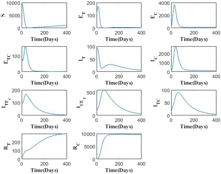
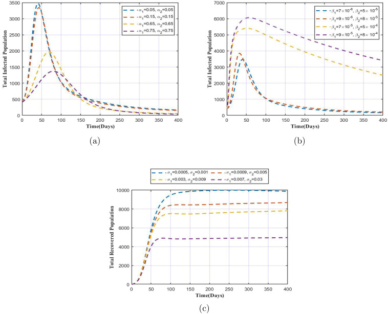
The model solution is presented in Fig. 2, from which we observe the variation in each variable over a time period of 400 days. The parameter values are as in Table 1. Fig. 3 represents the variation in total infected and total recovered population with increase or decrease in the respective parameter values. In Fig. 3, we showcase the impact of simultaneous change key parameters on the total infected and recovered population. Fig. 3(a) clearly signifies importance of the face mask factor in reducing the number of infections. We note that with increase in the values of ${\alpha }_1$ and ${\alpha }_2$ by greater margin, there is a huge fall in the total number of infected population. Use of face mask efficiently will help control the spread or virus in case of COVID-19 as well as the TB bacilli suspended in air in the form of droplet significantly. Fig. 3(b) shows that with increase in infection rates, the spread will be accelerated as higher infection rate imply occurrence of more effective contacts with infectious individuals. This needs to be taken seriously as this situation demands implementation of necessary interventions to reduce the spread of infection. Fig. 3(c) shows that if the immunity wanes quickly, the recoveries will reduce as this suggests that after recovery, the individuals soon become susceptible towards the disease again.

Fig. 2.

Solution curves of the TB-COVID-19 co-infection model.

Fig. 3.

Variation in total infected population with respect to (a) ${\alpha }_1,{\alpha }_2$, (b) ${\beta }_1,{\beta }_2$, and variation in total recovered population with respect to (c) ${\sigma }_1,{\sigma }_2$.

Table 1.

Model parameters.

Parameters	Meaning	Value	Reference
$\wedge$	Recruitment rate	5	Varies
${\alpha }_1$	TB Mask usage parameter	[0,1]	Varies
${\alpha }_2$	COVID-19 Mask usage parameter	0.05	[19], [34]
${\sigma }_1$	Waning rate from $R_T$ to $S$	0.0005	Assumed
${\sigma }_2$	Waning rate from $R_C$ to $S$	0.001	Assumed
${\delta }_1$	Rate at which TB exposed become TB infectious	[0.01,0.071]	[46], [47]
${\delta }_2$	Rate at which COVID-19 exposed become COVID-19 infectious	[0.071,0.33]	[29], [31]
${\zeta }_1$	Progression from $E_{TC}$ to $I_{T{E}_C}$	0.01	Assumed
${\zeta }_2$	Progression from $E_{TC}$ to $I_{C{E}_T}$	0.07	Assumed
${\eta }_1$	Rate at which co-infected individuals ($I_{TC}$) recover from COVID-19 only	0.0714	[44], [54]
${\eta }_2$	Rate at which co-infected individuals ($I_{TC}$) recover from TB only	[0.004,0.07]	[46], [47]
${\epsilon }_1$	Factor that enhances acquiring of COVID-19 infection after being infected with TB	1.5	Assumed
${\epsilon }_2$	Factor that enhances acquiring of TB infection after being infected with COVID-19	1.1	Assumed
${\gamma }_1$	Recovery rate of $I_T$	[0.004,0.07]	[46], [47]
${\gamma }_2$	Recovery rate of $I_C$	0.0714	[44], [54]
${\xi }_1$	Progression from $I_{T{E}_C}$ to $I_{TC}$	0.033	Assumed
${\xi }_2$	Progression from $I_{C{E}_T}$ to $I_{TC}$	0.033	Assumed
${\mu }_1$	Death rate of $I_T$	$0.69\times 10^{-4}$	Assumed
${\mu }_2$	Death rate of $I_C$	$0.8\times 10^{-4}$	Assumed
${\mu }_3$	Death rate of $I_{T{E}_C}$	$0.7\times 10^{-4}$	Assumed
${\mu }_4$	Death rate of $I_{C{E}_T}$	$0.9\times 10^{-4}$	Assumed
${\mu }_5$	Death rate of $I_{TC}$	$0.9\times 10^{-4}$	Assumed
$\mu$	Natural death rate	0.0000425	Demographic

4.1. Sensitivity analysis

In this section we illustrate sensitivity analysis by means of forward sensitivity index [15] of the basic reproduction number ($R_0$) as well as we apply the approach of LHS-PRCC (i.e. Latin Hypercube Sampling - Partial Rank Correlation Coefficient) [11], [32] on our model given by Eqs. (1)–(11) to study the influence on different infected population class of different parameters involved in the model. In the study [28], the authors worked on global dynamics of a HTLV-I infection model and have performed detailed sensitivity analysis by means of normalized forward sensitivity index to bring out the relative significance of certain parameters in disease transmission. Basic reproduction number ($R_0$) is very crucial in signifying the number the secondary cases arising from a single infected primary case and checks on whether the situation is under control or not. The normalized forward sensitivity index of a variable with respect to a parameter is the ratio of the relative change in the variable to the relative change in the parameter [15]. Therefore, if for say $b$ represents a parameter, then the normalized forward sensitivity index of $R_0$ with respect to $b$ is given by

$$r_b^{R_0}=\frac{\partial R_0}{\partial b}\times \frac{b}{R_0}.$$

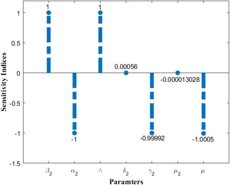
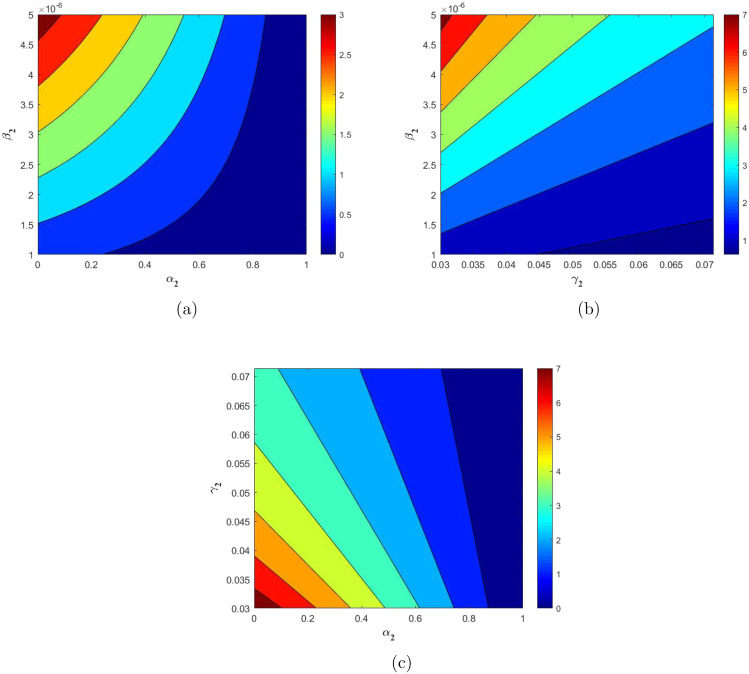
From Fig. 4 we note that $R_0$ shares negative indices with ${\alpha }_2$ and ${\gamma }_2$ and positive indices with $\wedge$ and ${\beta }_2$. This implies the negative and positive correlation with the former and latter parameters respectively. This indicates that if larger fraction of population is using the mask efficiently then the spread of virus and the bacteria can be diminished. Higher recovery rates directly imply a shorter infectious period, which further suggests that period to make effective contacts is less, thereby reduction in the spread of infection and hence the basic reproduction number. In Fig. 4, the sensitivity indices respective to each parameter. These indices values further suggest that if there is a 10% increase in infection rate (${\beta }_2$), then there will be a rise in the $R_0$ value by 10% as the respective index value is 1 for this parameter. In a similar way we note that the $r_{{\gamma }_2}^{R_0}=-0.99992$. This implies that a 10% increase in the recovery rate (${\gamma }_2$) will decrease the $R_0$ by 9.9992%. Similarly it applies to the remaining set of parameters. In a similar context, we study the impact of two parameters at once on the basic reproduction number ($R_0$)in Fig. 5. Fig. 5(a) shows that with the increase in the infection rate (${\beta }_2$), the $R_0$ value increases and it decreases with increase in ${\alpha }_2$ value. Fig. 5(b) shows a similar behaviour with ${\beta }_2$ and ${\gamma }_2$. In Fig. 5(c) we clearly witness the decrease in the $R_0$ value with increase in face mask factor (${\alpha }_2$) and recovery rate (${\gamma }_2$) values. This is evident as higher recovery rates implies shorter infectious period and thereby implying lesser chances of disease transmission. We obtain for a specific range of these parameters, the $R_0$ value can be brought below 1. The analysis on reproduction number is crucial as $R_0$ value is highly significant in determining the state of an epidemic. The value greater than 1 implies widespread of the disease in an uncontrolled manner. Hence from these two illustrations we conclude that usage of face mask correctly and efficiently will help in bringing down the basic reproduction number value thereby reducing the spread of disease vastly.

Fig. 4.

Normalized forward sensitivity index of the basic reproduction number of the TB-COVID-19 co-infection model. The parameter values are as in Table 1.

Fig. 5.

Contour plots showing the effect of (a) ${\beta }_2,{\alpha }_2$, (b) ${\beta }_2,{\gamma }_2$, and (c) ${\gamma }_2,{\alpha }_2$ on the basic reproduction number.

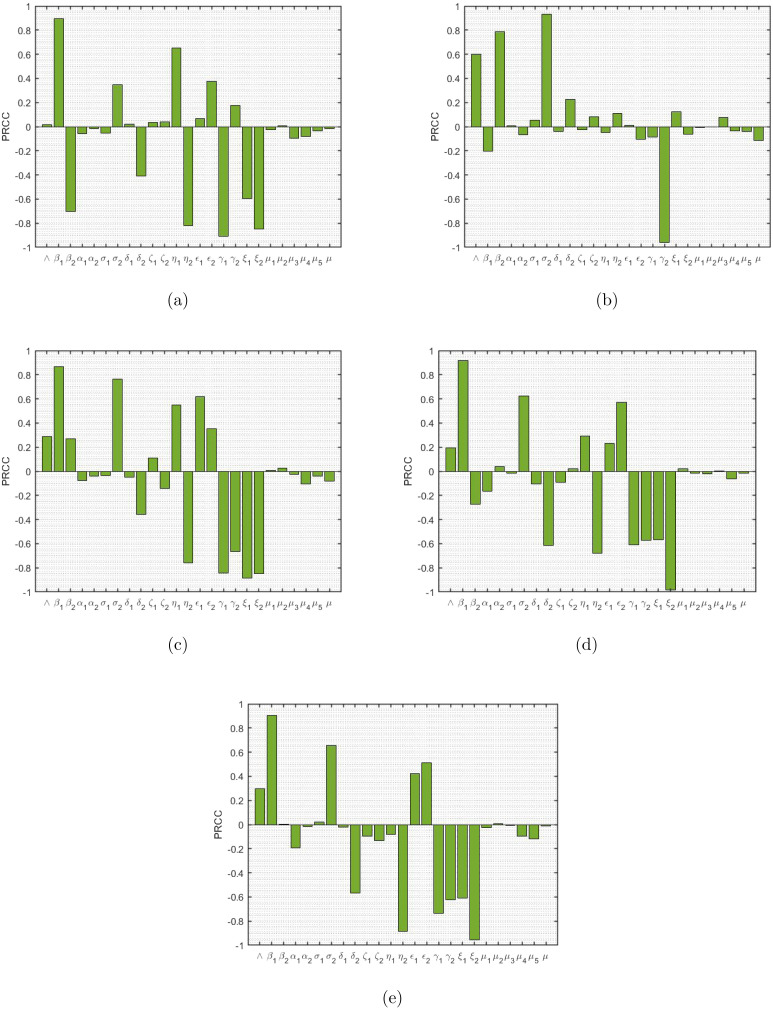
Sensitivity analysis following the approach of Latin Hypercube Sampling and Partial Rank Correlation Coefficient is employed to understand the complete parameter space on the different infected population variables of the model, and is illustrated in Fig. 6. The parameters are assumed to be uniformly distributed and the different response functions considered to perform the analysis are $I_T,I_C,I_{T{E}_C},I_{C{E}_T},\text{and}{I}_{TC}$. The effectiveness of this approach is tested by determining the PRCC values and further examining the sensitivity of the parameters of the developed model. To get the PRCC values, at first Latin Hypercube Sampling (LHS) method is applied to stratify the sample without replacement. This is followed by setting the baseline values of the parameters and then the simulations are carried out for PRCC analysis. The set parameter values range between $\pm 25\text{\%}$ from the baseline value which are listed in Table 2, and the simulations are run for 500 days per LHS.

Fig. 6.

PRCC results showing sensitivity indices of the model parameters with (a) TB only infected ($I_T)$, (b) COVID-19 only infected ($I_C$), (c) TB infected COVID-19 exposed ($I_{T{E}_C}$), (d) COVID-19 infected TB exposed ($I_{C{E}_T}$), and (e) TB and COVID-19 co-infected ($I_{TC}$).

The PRCC value for each parameter corresponding to the respective response function is provided in Table 2. The magnitude as well as the direction of PRCC values of the distinct parameters are of prime importance in determining a respective parameter’s contribution in model prediction and level of exactness. The PRCC values which are greater than 0.5 (closer to 1) and lesser than $-0.5$ (closer to $-1$) are quite important [45], as this implies stronger influence of LHS parameter on the outcome measure. From the Fig. 6, we clearly notice that the parameters ${\beta }_1,{\beta }_2,{\gamma }_1,{\gamma }_2,{\eta }_{,}{\eta }_2,{\epsilon }_1,{\epsilon }_2,{\xi }_1,{\xi }_2,{\sigma }_2,{\delta }_1,{\delta }_2$ are having a stronger influence on each of the infected population considered. It is clearly observed that TB infection rate (${\beta }_1$) has PRCC values very close to 1, signifying a higher level uncertainties or variations in infected population ($I_T,I_{T{E}_C},I_{C{E}_T}$ and $I_{TC}$) with change in its values. Surely, in case of the COVID-19 only infected population, the respective ${\beta }_2$ PRCC value is closer to 1 signifying a strong positive correlation. The similar explanation goes for the other such significant parameters. We observe that the recovery rates ${\gamma }_1$ and ${\gamma }_2$, and the enhancement factors ${\epsilon }_1,{\epsilon }_2$ and ${\epsilon }_3$ have negative and positive PRCC values respectively with respect to the exposed and co-infected population $I_{T{E}_C},I_{C{E}_T}$ and $I_{TC}$. We also note that in each of these figures, either one of the parameters ${\alpha }_1$ and ${\alpha }_2$ or both which signify product of face mask efficacy and fraction of population wearing it precisely, have negative PRCC values with respect to each infected population class, thereby signifying the crucial role of correct face mask usage in reduction of infections. The progression rates ${\delta }_1$ and ${\delta }_2$ are quite significant, since their values are either greater than 0.5 or lesser that $-0.5$, suggesting higher level of uncertainty in the rise and fall of the infected cases. Overall, we observe that the correlation between the respective variable and the parameter based on PRCC values, justifies with the respective model equations.

Table 2.

PRCC values of the model parameters.

Parameters	Baseline value	Range	PRCC ($I_T$)	PRCC ($I_C$)	PRCC ($I_{T{E}_C}$)	PRCC ($I_{C{E}_T}$)	PRCC ($I_{TC}$)
$\wedge$	2	1.5–2.5	0.0158	0.5987	0.2875	0.1962	0.2968
${\beta }_1$	$7\times 10^{-6}$	$5.25\times 10^{-6}$–$8.75\times 10^{-6}$	0.8960	−0.2017	0.8655	0.9202	0.9060
${\beta }_2$	$5\times 10^{-5}$	$3.75\times 10^{-5}$–$6.25\times 10^{-5}$	−0.7046	0.7854	0.2692	−0.2717	0.0020
${\alpha }_1$	0.05	0.0375–0.0625	−0.0567	0.0059	−0.0759	−0.1636	−0.1950
${\alpha }_2$	0.05	0.0375–0.0625	−0.0152	−0.0661	−0.0387	0.0402	−0.0156
${\sigma }_1$	0.0005	$3.75\times 10^{-4}$–$6.25\times 10^{-4}$	−0.0541	0.0519	−0.0368	−0.0178	0.0210
${\sigma }_2$	0.001	0.00075–0.0013	0.3499	0.9321	0.7623	0.6233	0.6571
${\delta }_1$	0.03	0.0225–0.0375	0.0227	−0.0410	−0.0481	−0.1052	−0.0189
${\delta }_2$	0.071	0.0532–0.0887	−0.4075	0.2250	−0.3565	−0.6160	−0.5699
${\zeta }_1$	0.01	0.0075–0.0125	0.0371	−0.0258	0.1113	−0.0902	−0.0950
${\zeta }_2$	0.07	0.0525–0.0875	0.0407	0.0816	−0.1442	0.0232	−0.1332
${\eta }_1$	0.04	0.03–0.05	0.6535	−0.0468	0.5468	0.2936	−0.0807
${\eta }_2$	0.0714	0.0536–0.0893	−0.8180	0.1113	−0.7595	−0.6782	−0.8872
${\epsilon }_1$	1.5	1.125–1.875	0.0681	0.0099	0.6170	0.2307	0.4251
${\epsilon }_2$	1.1	0.825–1.375	0.3765	−0.1046	0.3530	0.5742	0.5122
${\gamma }_1$	0.04	0.03–0.05	−0.9093	−0.0857	−0.8418	−0.6079	−0.7352
${\gamma }_2$	0.0714	0.0536–0.0893	0.1770	−0.9617	−0.6669	−0.5705	−0.6239
${\xi }_1$	0.033	0.0248–0.0413	−0.5962	0.1245	−0.8860	−0.5685	−0.6096
${\xi }_2$	0.01	0.0075–0.0125	−0.8501	−0.0614	−0.8481	−0.9849	−0.9549
${\mu }_1$	0.000069	$5.175\times 10^{-5}$–$8.625\times 10^{-5}$	−0.0267	−0.0055	0.0048	0.0225	−0.0234
${\mu }_2$	0.00008	$6\times 10^{-5}$–$1\times 10^{-4}$	0.0059	−0.0039	0.0256	−0.0151	0.0091
${\mu }_3$	0.00007	$5.25\times 10^{-5}$–$8.75\times 10^{-5}$	−0.0976	0.0787	−0.0238	−0.0197	−0.0077
${\mu }_4$	0.00009	$6.75\times 10^{-5}$–$1.125\times 10^{-4}$	−0.0828	−0.0372	−0.1033	0.0033	−0.0955
${\mu }_5$	0.00009	$6.75\times 10^{-5}$–$1.125\times 10^{-4}$	−0.0345	−0.0411	−0.0397	−0.0650	−0.1212
$\mu$	0.0000425	$3.1875\times 10^{-5}$–$5.3125\times 10^{-5}$	−0.0156	−0.1137	−0.0828	−0.0172	−0.0099

5. Optimal control

5.1. Optimal control problem

Optimal control analysis is of great importance in determining significant control strategies in infectious disease. As per the report by WHO [52], the TB care was reduced by 21% in low-income countries amid the COVID-19 pandemic. Since TB has a varied incubation as well as infectious period, in due time if treatment is provided and awareness is spread through counselling, risks related to chronic illness and development of COVID-19 disease along with TB can be avoided. It is also witnessed that COVID-19 can spread easily through the unidentified infectives. Therefore, it is of utmost significance for these exposed individuals to be isolated so that their contact with TB infectives can also be reduced. Being exposed to both of the diseases can be avoided if proper care is taken in controlling the spread of both diseases. Contemplating this, we include 2 control parameters in the TB-COVID-19 model represented by the system of Eqs. (1)–(11) which are:

• •$u_1$: This control relates to improved and early detection of the exposed COVID-19 individuals by setting up rigorous testing drives, investing on home testing kits, and isolation facilities. This control is incorporated with a vision towards reduction of exposed COVID-19 individuals coming in contact with TB infected patients. This could help in reducing the population from getting exposed to both the diseases.
• •$u_2$: This control relates towards improvement of TB recovery period. This is equated towards implementation of proper treatment and counselling policies for TB care, so that recovery period can be improved by providing right treatment and counselling at the initial stage, thereby reducing the negligence in taking treatment.

These two control functions are bounded and Lebesgue integrable on $[0,t_f]$, where $t_f$ is the pre-fixed time period to which these two controls are applied. It is assumed that $u_1$ and $u_2$ lie between 0 and 1, the reason being, if these two equal zero, it simply infers no efforts being placed in these controls. Similarly, utmost effort implies to these values being 1. As per the above explanation we include the two controls in the model (1)–(11) and obtain the following optimal control model:

$$\frac{dS}{dt}=\wedge +{\sigma }_1{R}_T+{\sigma }_2{R}_C-({\lambda }_T+{\lambda }_C+\mu )S$$ (17)

$$\frac{d{E}_T}{dt}={\lambda }_{T}S-({\delta }_1+{\lambda }_C+\mu )E_T$$ (18)

$$\frac{d{E}_C}{dt}={\lambda }_{C}S-({\delta }_2+{\lambda }_T(1-u_1\left(t\right))+\mu )E_C$$ (19)

$$\frac{d{E}_{TC}}{dt}={\lambda }_C{E}_T+{\lambda }_T(1-u_1\left(t\right))E_C-({\zeta }_1+{\zeta }_2+\mu )E_{TC}$$ (20)

$$\frac{d{I}_T}{dt}={\delta }_1{E}_T+{\eta }_1{I}_{TC}-({\epsilon }_1{\lambda }_C+{\mu }_1+\mu )I_T-({\gamma }_1+u_2\left(t\right))I_T$$ (21)

$$\frac{d{I}_C}{dt}={\delta }_2{E}_C+{\eta }_2{I}_{TC}-({\gamma }_2+{\epsilon }_2{\lambda }_T+{\mu }_2+\mu )I_C$$ (22)

$$\frac{d{I}_{T{E}_C}}{dt}={\epsilon }_1{\lambda }_C{I}_T+{\zeta }_1{E}_{TC}-({\xi }_1+{\mu }_3+\mu )I_{T{E}_C}$$ (23)

$$\frac{d{I}_{C{E}_T}}{dt}={\epsilon }_2{\lambda }_T{I}_C+{\zeta }_2{E}_{TC}-({\xi }_2+{\mu }_4+\mu )I_{C{E}_T}$$ (24)

$$\frac{d{I}_{TC}}{dt}={\xi }_1{I}_{T{E}_C}+{\xi }_2{I}_{C{E}_T}-({\eta }_1+{\eta }_2++{\mu }_5+\mu )I_{TC}$$ (25)

$$\frac{d{R}_T}{dt}=({\gamma }_1+u_2\left(t\right))I_T-({\sigma }_1+\mu )R_T$$ (26)

$$\frac{d{R}_C}{dt}={\gamma }_2{I}_C-({\sigma }_2+\mu )R_C,$$ (27)

where

$${\lambda }_T={\beta }_1(1-{\alpha }_1)(I_T+I_{TC}+I_{T{E}_C})\text{and}{\lambda }_C={\beta }_2(1-{\alpha }_2)(I_C+I_{TC}+I_{C{E}_T})$$

The objective functional for the fixed $t_f$ is given by

$$J={\int }_0^{t_f}{C}_1{I}_T+C_2{I}_C+C_3{I}_{T{E}_C}+C_4{I}_{C{E}_T}+C_5{I}_{TC}+\frac{1}{2}{C}_6{u}_1^2+\frac{1}{2}{C}_7{u}_2^2,$$ (28)

where $C_1,C_2,C_3,C_4,C_5,C_6,C_7\ge 0$ are the weight constants.

Objective is to find the control parameters $u_1\ast$, $u_2\ast$ such that

$$J(u_1\ast ,u_2\ast )=\underset{u_1,u_2\in \Omega }{min}J(u_1,u_2)$$ (29)

where $\Omega$ is the control set, defined as

$$\Omega =\left\{u_1,u_2:\text{measurable}\text{and}0\le u_1,u_2<1\right\}andt\in [0,t_f]$$

The Lagrangian of this problem is:

$$L(I_T,I_C,I_{T{E}_C},I_{C{E}_T},I_{TC},u_1,u_2)=C_1{I}_T+C_2{I}_C+C_3{I}_{T{E}_C}+C_4{I}_{C{E}_T}+C_5{I}_{TC}+\frac{1}{2}{C}_6{u}_1^2+\frac{1}{2}{C}_7{u}_2^2$$

The Hamiltonian $\mathcal{H}$ formed for our problem is :

$$\mathcal{H}=(I_T,I_C,I_{T{E}_C},I_{C{E}_T},I_{TC},u_1,u_2)+{\lambda }_1\frac{dS}{dt}+{\lambda }_2\frac{d{E}_T}{dt}+{\lambda }_3\frac{d{E}_C}{dt}+{\lambda }_4\frac{d{E}_{TC}}{dt}+{\lambda }_5\frac{d{I}_T}{dt}+{\lambda }_6\frac{d{I}_C}{dt}+{\lambda }_7\frac{d{I}_{T{E}_C}}{dt}+{\lambda }_8\frac{d{I}_{C{E}_T}}{dt}+{\lambda }_9\frac{d{I}_{TC}}{dt}+{\lambda }_{10}\frac{d{R}_T}{dt}+{\lambda }_{11}\frac{d{R}_C}{dt}$$

where ${\lambda }_i^{\prime }s$ are the adjoint variables (i $=$ 1 to 11). The adjoint variables are written in the form of differential equations as follows:

$$\frac{d{\lambda }_1}{dt}=-\frac{\partial \mathcal{H}}{\partial S}=({\lambda }_1-{\lambda }_2){\beta }_1(1-{\alpha }_1)(I_T+T_{TC}+I_{T{E}_C})+({\lambda }_1-{\lambda }_3){\beta }_2(1-{\alpha }_2)(I_C+T_{TC}+I_{C{E}_T})$$

$$+{\lambda }_1\mu$$ (30)

$$\frac{d{\lambda }_2}{dt}=-\frac{\partial \mathcal{H}}{\partial E_T}=({\lambda }_2-{\lambda }_4){\beta }_2(1-{\alpha }_2)(I_C+T_{TC}+I_{C{E}_T})+({\lambda }_2-{\lambda }_5){\delta }_1+{\lambda }_2\mu$$ (31)

$$\frac{d{\lambda }_3}{dt}=-\frac{\partial \mathcal{H}}{\partial E_C}=({\lambda }_3-{\lambda }_4)(1-u_1\left(t\right)){\beta }_1(1-{\alpha }_1)(I_T+T_{TC}+I_{T{E}_C})+({\lambda }_3-{\lambda }_6){\delta }_2+{\lambda }_3\mu$$ (32)

$$\frac{d{\lambda }_4}{dt}=-\frac{\partial \mathcal{H}}{\partial E_{TC}}=({\lambda }_4-{\lambda }_7){\zeta }_1+({\lambda }_4-{\lambda }_8){\zeta }_2+{\lambda }_4\mu$$ (33)

$$\frac{d{\lambda }_5}{dt}=-\frac{\partial \mathcal{H}}{\partial I_T}=-C_1+({\lambda }_1-{\lambda }_2){\beta }_1(1-{\alpha }_1)S+({\lambda }_3-{\lambda }_4){\beta }_1(1-{\alpha }_1)(1-u_1\left(t\right))E_C+({\lambda }_5-{\lambda }_{10})({\gamma }_1+u_2\left(t\right))+({\lambda }_5-{\lambda }_7){\epsilon }_1{\beta }_2(1-{\alpha }_2)(I_C+T_{TC}+I_{C{E}_T})+({\lambda }_6-{\lambda }_8){\epsilon }_2{\beta }_1(1-{\alpha }_1)I_C+{\lambda }_5({\mu }_1+\mu )$$ (34)

$$\frac{d{\lambda }_6}{dt}=-\frac{\partial \mathcal{H}}{\partial I_C}=-C_2+({\lambda }_1-{\lambda }_3){\beta }_2(1-{\alpha }_2)S+({\lambda }_2-{\lambda }_4){\beta }_2(1-{\alpha }_2)E_T+({\lambda }_6-{\lambda }_{11}){\gamma }_2+({\lambda }_5-{\lambda }_7){\epsilon }_1{\beta }_2(1-{\alpha }_2)I_T+({\lambda }_6-{\lambda }_8){\epsilon }_2{\beta }_1(1-{\alpha }_1)(I_T+I_{TC}+I_{T{E}_C})+{\lambda }_6({\mu }_2+\mu )$$ (35)

$$\frac{d{\lambda }_7}{dt}=-\frac{\partial \mathcal{H}}{\partial I_{T{E}_C}}=-C_3+({\lambda }_1-{\lambda }_2){\beta }_1(1-{\alpha }_1)S+({\lambda }_3-{\lambda }_4){\beta }_1(1-{\alpha }_1)(1-u_1\left(t\right))E_C+({\lambda }_6-{\lambda }_8){\epsilon }_2{\beta }_1(1-{\alpha }_1)I_C+({\lambda }_7-{\lambda }_9){\xi }_1+{\lambda }_7({\mu }_3+\mu )$$ (36)

$$\frac{d{\lambda }_8}{dt}=-\frac{\partial \mathcal{H}}{\partial I_{C{E}_T}}=-C_4+({\lambda }_1-{\lambda }_3){\beta }_2(1-{\alpha }_2)S+({\lambda }_2-{\lambda }_4){\beta }_2(1-{\alpha }_2)E_T+({\lambda }_8-{\lambda }_9){\xi }_2+({\lambda }_5-{\lambda }_7){\epsilon }_1{\beta }_2(1-{\alpha }_2)I_T+{\lambda }_8({\mu }_4+\mu )$$ (37)

$$\frac{d{\lambda }_9}{dt}=-\frac{\partial \mathcal{H}}{\partial I_{TC}}=-C_5+({\lambda }_1-{\lambda }_2){\beta }_1(1-{\alpha }_1)S+({\lambda }_1-{\lambda }_3){\beta }_2(1-{\alpha }_2)S+({\lambda }_3-{\lambda }_4){\beta }_1(1-{\alpha }_1)(1-u_1\left(t\right))E_C+({\lambda }_2-{\lambda }_4){\beta }_2(1-{\alpha }_2)E_T+({\lambda }_5-{\lambda }_7){\epsilon }_1{\beta }_2(1-{\alpha }_2)I_T+({\lambda }_6-{\lambda }_8){\epsilon }_2{\beta }_1(1-{\alpha }_1)I_C+({\lambda }_5-{\lambda }_9){\eta }_1+({\lambda }_6-{\lambda }_9){\eta }_2+{\lambda }_9({\mu }_5+\mu )$$ (38)

$$\frac{d{\lambda }_{10}}{dt}=-\frac{\partial \mathcal{H}}{\partial R_T}=({\lambda }_{10}-{\lambda }_1){\sigma }_1+{\lambda }_{10}\mu$$ (39)

$$\frac{d{\lambda }_{11}}{dt}=-\frac{\partial \mathcal{H}}{\partial R_C}=({\lambda }_{11}-{\lambda }_1){\sigma }_2+{\lambda }_{11}\mu$$ (40)

Let $\tilde{S},\widetilde{E_T},\widetilde{E_C},\widetilde{E_{TC}},\widetilde{I_T},\widetilde{I_C},\widetilde{I_{T{E}_C}},\widetilde{I_{C{E}_T}},\widetilde{I_T},\widetilde{R_T},\widetilde{R_C}$ be optimum values of $S,E_T,E_C,E_{TC}$, $I_T,I_C,I_{T{E}_C},I_{C{E}_T},I_{TC},R_T,\text{and}{R}_C$ respectively. Let $\widetilde{{\lambda }_1},\widetilde{{\lambda }_2},\widetilde{{\lambda }_3},\widetilde{{\lambda }_4},\widetilde{{\lambda }_5},\widetilde{{\lambda }_6},\widetilde{{\lambda }_7},\widetilde{{\lambda }_8},\widetilde{{\lambda }_9},\widetilde{{\lambda }_{10}}$, and $\widetilde{{\lambda }_{11}}$ be solution of system of Eqs. (30)–(40). By using [30], [36], [37] we state and prove the below theorem.

Theorem 5.1

There exist optimal controls$u_1\ast$,$u_2\ast$$\in \Omega$such that$J(u_1\ast ,u_2\ast )=minJ(u_1,u_2)$subject to extended system of Eqs. (17) – (27) .

Proof

We use [37] to prove this theorem. In this case, we observe that the controls are non-negative. The necessary convexity of the objective functional in $(u_1,u_2)$ is satisfied for minimizing the problem. The set of control variable, $u_1,u_2\in \Omega$ is convex and closed by definition. The state variables are bounded and the integrand of the functional $C_1{I}_T+C_2{I}_C+C_3{I}_{T{E}_C}+C_4{I}_{C{E}_T}+C_5{I}_{TC}+\frac{1}{2}{C}_6{u}_1^2+\frac{1}{2}{C}_7{u}_2^2$ is convex on $\Omega$. Since there exist optimal controls for minimizing the functional subject to systems (17)–(27), (30)–(40), we use Pontryagin’s maximum principle [37] to derive the necessary conditions to find the optimal solutions in the following way: Suppose $(z,u)$ is an optimal solution of an optimal control problem, then this implies that there exists a non-trivial vector function $\lambda ={\lambda }_1,{\lambda }_2,\dots ,{\lambda }_n$ satisfying the following:

$$\frac{dz}{dt}=\frac{\partial \mathcal{H}(t,z,u,\lambda )}{\partial \lambda },0=\frac{\partial \mathcal{H}(t,z,u,\lambda )}{\partial u}\text{at}u\ast ,\frac{d\lambda }{dt}=-\frac{\partial \mathcal{H}(t,z,u,\lambda )}{\partial z}$$

Theorem 5.2

The optimal controls $u_1\ast$ , $u_2\ast$ which minimize $J$ over the region $\Omega$ is given by:

$$u_1\ast =min\left\{1,max(0,\widetilde{u_1})\right\}\text{and}{u}_2\ast =min\left\{1,max(0,\widetilde{u_2})\right\},$$

where

$$\widetilde{u_1}=\frac{({\lambda }_3-{\lambda }_4){\beta }_1(1-{\alpha }_1)(I_T+I_{TC}+T_{T{E}_C})E_C}{C_6}\text{and}\widetilde{u_2}=\frac{({\lambda }_5-{\lambda }_{10})I_T}{C_7}$$

Proof

We prove this theorem by using [36], [37] and Theorem 5.1.

Using the optimally condition: $\frac{\partial \mathcal{H}}{\partial u_1}=0$, $\frac{\partial \mathcal{H}}{\partial u_2}=0$ we get,

$$\frac{\partial \mathcal{H}}{\partial u_1}=C_6{u}_1+({\lambda }_3-{\lambda }_4){\beta }_1(1-{\alpha }_1)(I_T+I_{TC}+T_{T{E}_C})E_C=0⟹u_1=\frac{({\lambda }_3-{\lambda }_4){\beta }_1(1-{\alpha }_1)(I_T+I_{TC}+T_{T{E}_C})E_C}{C_6}=\widetilde{u_1}\text{and}\frac{\partial \mathcal{H}}{\partial u_2}=C_7{u}_2+({\lambda }_5-{\lambda }_{10})I_T=0⟹u_2=\frac{({\lambda }_5-{\lambda }_{10})I_T}{C_7}=\widetilde{u_2}$$

Again the lower bound is 0 and upper bound is 1 for the controls $u_1$ and $u_2$. This suggests that $u_1=u_2=0$ if $\widetilde{u_1}<0$ and $\widetilde{u_2}<0$, also $u_1=u_2=1$ if $\widetilde{u_1}>1$ and $\widetilde{u_2}>1$, otherwise $u_1=\widetilde{u_1}$ and $u_2=\widetilde{u_2}$. Therefore, for these controls $u_1\ast$ and $u_2\ast$ we get optimum values of $J$.

5.2. Optimal control model simulation

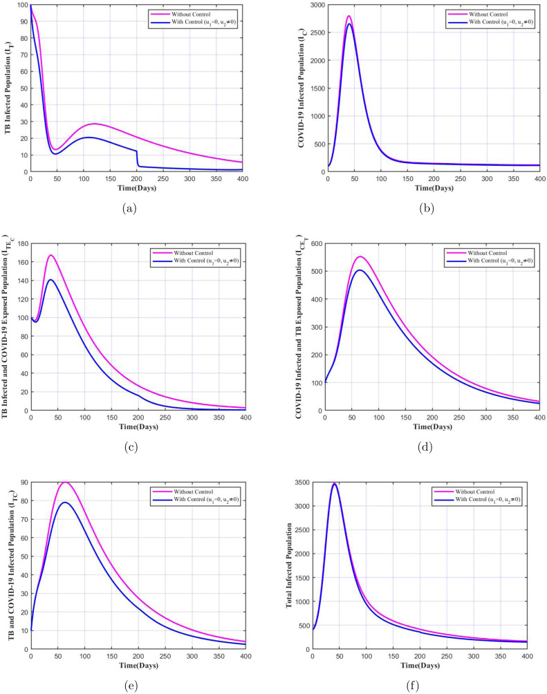
In this section we perform simulations for a period of 400 days and illustrate analytical results using MATLAB software, by setting the parameter values as in Table 1. The extended system of Eqs. (17)–(27) is solved applying iterative method using forward and backward difference approximation as in [30]. The forward difference approximation is applied to first solve the state equations (17)–(27), and then applying the backward difference approximation, the adjoint equations (30)–(40) are solved. The positive valued constants $C_1,C_2,C_3,C_4,C_5$ are the weight constants which represent the weight which balance offs the TB only infected population, COVID-19 only infected population, TB infected COVID-19 exposed population, COVID-19 infected TB exposed population, and co-infected population to both the diseases respectively. The positive constants $C_6,\text{and}{C}_7$ represent the weight constants for improved testing and TB treatment, counselling respectively. The values assigned to the weight constants are $C_1=1,C_2=1,C_3=1,C_4=1,C_5=1,C_6=100,\text{and}{C}_7=100$. The initial values assigned to the variables to perform the simulations are $S=10000,E_T=100,E_C=100,E_{TC}=100,I_T=100,I_C=100,I_{T{E}_C}=100,I_{C{E}_T}=100,I_{TC}=10,R_T=1,R_C=‘1$. In this section, the impact on control profile with variation in costs is studied. This is followed by studying the impact on the infected population with and without the two controls as well considering specifically one control at a time.

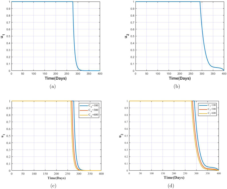
The illustration on the control profiles over time as well the impact on the same due to variation in costs is depicted in Fig. 7. It is clearly observed that the control $u_2$ needs to be maintained at 1 for longer time compared to that of control $u_1$, implying that significance of control $u_2$ is more compared to that of $u_1$. From Fig. 7(c) and (d) we observe that with the increase in the costs, the duration for which the control profile resides at 1 declines. This is justified, as higher costs in the means of providing testing kits, conducting testing drives, counselling and treatment facilities etc. call in for lesser duration of investments on those equipment and policies. In the coming section we see the variation in infected population with and without application of controls parameters, and provide a clarity on the significance of the controls individually as well as when applied together.

Fig. 7.

Control profile of (a) $u_1$, (b) $u_2$, (c) $u_1$ with variation in costs and (d) $u_2$ with variation in costs.

5.2.1. Optimal control simulation when both controls are applied

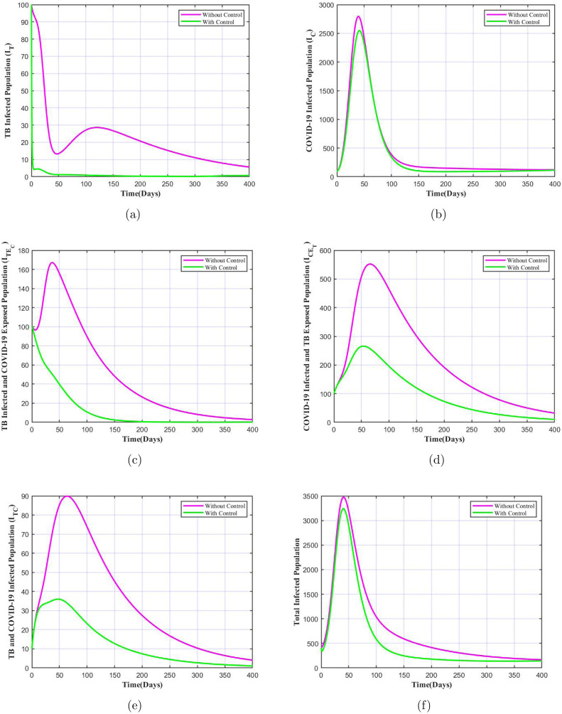
When both controls relating to enhanced detection and isolation (i.e. $u_1\ne 0$) and early TB treatment and counselling (i.e. $u_2\ne 0$) are applied, it results in significant difference in the number of infectives under the application of controls which is depicted in Fig. 8. We note that for each class of infected population there is huge decrease in the number of infectives when both controls are applied, and the number nears to zero in a shorter period of time, except for COVID-19 only infected population. In the later case there is a very small difference, since the controls focus on minimizing exposure to both diseases with major insistence on TB treatment. As per the report [52] and the study in [14], it is conveyed that the TB infected individuals, both latent TB patients as well as with TB disease are at increased risk of getting COVID-19 as well as the severity of the COVID-19 symptoms in these patients would be more. Hence, our optimal control model which was framed keeping this into consideration provides desired results, stressing on the importance of both the control parameters when implemented at once.

Fig. 8.

Variation in infected population with and without both the controls.

5.2.2. Optimal control simulation when exclusively one of the controls is applied

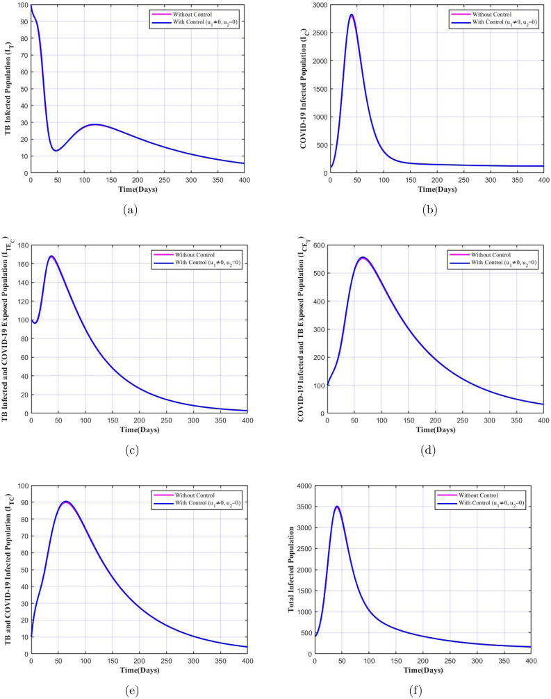
In the case when $u_1=0$ and only the control related to improved TB treatment and counselling $(u_2\ne 0)$ is applied we see that there is a considerable decline in the number of infectives of each class when the control is applied which is shown in Fig. 9. This suggests that the control $u_2$ is quite important in controlling the disease spread, since even when implemented alone it contributes towards reduction of infected cases. This is supported by the studies [14], [52] which suggests that TB infected patients are more vulnerable to COVID-19, implying higher individuals with dual infections. On the other hand, from the Fig. 10 we note that there is barely any difference in number of infectives with and without the control $u_1$. This suggests that without improved TB care ($u_2=0$) and mere detection and isolation of exposed COVID-19 individuals ($u_1\ne 0$) will not help in decline of co-infections, single disease infection or simultaneous infection from one disease and exposure to another disease as per our model. Though the control $u_1$ is not significant compared to the control $u_2$ when applied separately, however when both controls are applied at once we notice that the decline in number of infected population is much higher when mere one control is applied. Therefore, these simulations stress on the importance of both the controls in controlling spread of co-infections when implemented together.

Fig. 9.

Variation in infected population with TB treatment and counselling ($u_2\ne 0,u_1=0$) control only.

Fig. 10.

Variation in infected population with testing drives for detection of exposed COVID-19 cases ($u_1\ne 0,u_2=0$) control only.

6. Conclusion

In this work we performed a detailed study on the deterministic epidemiological model comprising of 11 compartments. The study began with a detailed analysis covering equilibria, basic reproduction number, stability and bifurcation analysis of the disease-free and endemic equilibrium. From the analysis on TB only model and COVID-19 only model we prove that the disease-free equilibrium and the endemic equilibrium are locally asymptotically stable when the respective basic reproduction numbers ($R_{0_T}$ and $R_{0_C}$) are less than 1 and greater than 1 respectively. It is concluded that backward bifurcation does not exist in both models by applying centre manifold theory as in [13]. We obtain 4 equilibria for the TB - COVID-19 complete model, which are the disease-free equilibrium point, TB only equilibrium point, COVID-19 only equilibrium point and TB - COVID-19 co-existence endemic equilibrium point. The stability and bifurcation analysis are shown which prove the non-existence of backward bifurcation at $R_0=1$. These theoretical results are then followed by numerical simulations, sensitivity analysis and optimal control analysis.

Time series behaviour of the total infected and total recovered population for a period of 400 days is studied with respect to variation in two parameters at once, and it is witnessed that with increase in face mask efficacy and fraction of population wearing it precisely, the infection spread can be curbed. On the other hand, if the immunity wanes quickly, the recovered individuals move to being susceptible and hence at risk of infections. We note that with increase in recovery rates, the number of infected reduces, since smaller recovery implies shorter infectious period thereby nullifying the chance of spreading infections. Similarly, the impact of recovery rate, infection rate and face mask factor on the basic reproduction number is illustrated through sensitivity analysis and similar results are obtained. Using LHS-PRCC approach the significance and correlation of all the parameters with their respective response functions which in our case of study were the different infected population classes were obtained and analysed based on the PRCC values.

Optimal control analysis was then performed by including two control parameters, one is the enhanced detection and isolation ($u_1\left(t\right)$) and the other is early TB treatment and counselling (i.e. $u_2\left(t\right)$). A significant difference in the number of infectives under the application of controls was witnessed in the illustration. The effect of these controls individually was also performed and when compared, the control $u_2\left(t\right)$ served to be more important than $u_1\left(t\right)$, but when applied together, the reduction in the number of infected population was quite huge. Therefore, going by the study in [14] and the report by WHO [52] both latent TB patients as well as with TB disease are at increased risk of getting COVID-19. The controls which were included in the study provided desired results so as to combat the challenge of co-infection of these disease spread. Hence, this analysis focused on the need of improved TB treatment and care as well as enhanced testing and isolation facilities for COVID-19 exposed population to combat the unforeseen spread of two deadly diseases. Hence, the results from the study implies acceleration in the disease spread if proper treatment and care for TB infectives is neglected and detection, isolation facilities are not implemented. On a concluding note, the study further suggests that in the times of a pandemic, other chronic diseases, specifically the ones which spread through close contacts must not be neglected and adequate care has to be taken so that mortality due to co-infection and unavailability of timely treatment can be avoided.

Declaration of Competing Interest

The authors declare that they have no known competing financial interests or personal relationships that could have appeared to influence the work reported in this paper.

Appendix.

Theorem A.1 Castillo-Chavez and Song —

Consider the following general system of ordinary differential equations with a parameter $\varphi$ :

$$\frac{dx}{dt}=f(x,\varphi ),f:{\mathbb{R}}^n\times \mathbb{R}\to \mathbb{R}\text{and}{C}^2({\mathbb{R}}^n\times \mathbb{R})$$ (41)

where 0 is an equilibrium point of the system that is, $f(0,\varphi )\equiv 0$ for all $\varphi$ and assume

• 1. $A=D_{x}f(0,0)=\left(\frac{\partial f_i}{\partial x_j}(0,0)\right)$ is the linearization matrix of system (2) around the equilibrium 0 and $\varphi$ evaluated at 0. Zero is a simple eigenvalue of A and other eigenvalues of A have negative real parts;
• 2.
  Matrix A has a right eigenvector $W$ and a left eigenvector $V$ (each corresponding to the zero eigenvalue); Let $f_k$ be the $k$ th component of $f$ and

  $$a=\sum _{k,j,i=1}^n{v}_k{w}_i{w}_j\frac{{\partial }^2{f}_k}{\partial x_i\partial x_j}(0,0),b=\sum _{k,i=1}^n{v}_k{w}_i\frac{{\partial }^2{f}_k}{\partial x_i\partial \varphi }(0,0)$$

The local dynamics of the system around 0 is totally determined by the signs of $a$ and $b$ .

• 1. $a>0,b>0$ . When $\varphi <0$ with $\mid \varphi \mid \ll 1$ , 0 is locally asymptotically stable and there exists a positive unstable equilibrium; when $0<\varphi \ll 1$ , 0 is unstable and there exists a negative, locally asymptotically stable equilibrium;
• 2. $a<0,b<0$ . When $\varphi <0$ with $\mid \varphi \mid \ll 1$ , 0 is unstable; when $0<\varphi \ll 1$ , 0 is locally asymptotically stable and there exists a positive unstable equilibrium;
• 3. $a>0,b<0$ . When $\varphi <0$ with $\mid \varphi \mid \ll 1$ , 0 is unstable and there exists a locally asymptotically stable negative equilibrium; when $0<\varphi \ll 1$ , 0 is stable and a positive unstable equilibrium appears;
• 4. $a〈0,b〉0$ . When $\varphi$ changes from negative to positive, 0 changes its stability from stable to unstable. Correspondingly a negative unstable equilibrium becomes positive and locally asymptotically stable.