Tuberculosis detection in chest radiograph using convolutional neural network architecture and explainable artificial intelligence

Abstract

In most regions of the world, tuberculosis (TB) is classified as a malignant infectious disease that can be fatal. Using advanced tools and technology, automatic analysis and classification of chest X-rays (CXRs) into TB and non-TB can be a reliable alternative to the subjective assessment performed by healthcare professionals. Thus, in the study, we propose an automatic TB detection system using advanced deep learning (DL) models. A significant portion of a CXR image is dark, providing no information for diagnosis and potentially confusing DL models. Therefore, in the proposed system, we use sophisticated segmentation networks to extract the region of interest from multimedia CXRs. Then, segmented images are fed into the DL models. For the subjective assessment, we use explainable artificial intelligence to visualize TB-infected parts of the lung. We use different convolutional neural network (CNN) models in our experiments and compare their classification performance using three publicly available CXR datasets. EfficientNetB3, one of the CNN models, achieves the highest accuracy of 99.1%, with a receiver operating characteristic of 99.9%, and an average accuracy of 98.7%. Experiment results confirm that using segmented lung CXR images produces better performance than does using raw lung CXR images.

Introduction

Several diseases are considered life-threatening. These diseases are separated into different levels, with the riskiest diseases having a higher level. Risk factors depend on the disease and how it affects human life [1]. Some of these diseases are caused by different types of bacteria, viruses, fungi, and parasites. The respiratory system is considered one of the major systems of the human body. The respiratory system is important for many reasons [2]. Humans can breathe using the respiratory system to exchange carbon dioxide for oxygen through inhalation and exhalation. The primary organs of the respiratory system are the lungs, which perform this exchange of gases as we breathe. Many diseases endanger the respiratory system, interfering with its function [3]. One of these critical diseases is tuberculosis (TB) [1, 2, 4–10, 12–22]. TB is caused by a bacterium called Mycobacterium tuberculosis [1, 7]. Normally, the bacterium invades the lungs, reducing the efficiency of lung functions. It can also cause damage to other parts of the body such as the brain or spine [16]. TB is considered life-threatening based on the World Health Organization (WHO). According to the WHO, the number of deaths caused by TB has increased yearly [1–6, 8–11]. In 2019, there were 3.2 million men and 1.2 million women and children who tested positive for TB globally.

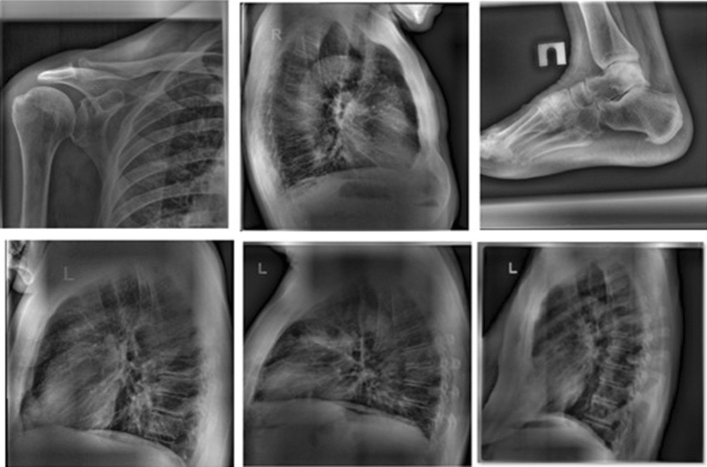
TB can be active or latent. The TB bacterium is present in both cases, so patients with the TB bacterium in their bodies have a common issue. However, in some cases of active TB, the body rejects the TB bacterium. This happens when the immune system is weakened because of illness or the use of certain medications. Hence, the TB bacterium has a favorable environment in which to replicate and cause symptoms. When the TB bacterium replicates, patients can spread the infection. Thus, doctors must provide medical treatment to patients with active TB. When TB is diagnosed in its early stages, it leads to earlier treatment initiation, a shorter period of infectiousness, and improved patient outcomes [2]. Active cases are risky, and early detection is key. Doctors will examine patients’ history and determine whether they are susceptible to developing TB. Doctors are usually familiar with TB symptoms. During a medical examination, doctors will notice that a patient with TB has a cough. This type of cough produces phlegm and causes fatigue and, in some cases, loss of weight as a result of a loss of appetite. Once doctors notice TB symptoms in a patient, they will ask the patient for a chest X-ray (CXR), which is performed by a radiographer [8, 23]. Electromagnetic radiation is the energy type produced by the movement of electrically charged particles moving through a matter or vacuum or by magnetic and electrical disturbance oscillating. Electromagnetic radiation can reach long distances in space and can pass through the body. In addition, X-ray types are based on the view as well as the starting and finishing points. The most common two types of X-ray are frontal and lateral; therefore, the input can be multi-dimensional. Figure 1 explains the differences between the X-ray types. The frontal includes two types, which are the posteroanterior (PA) and anteroposterior.

Fig. 1.

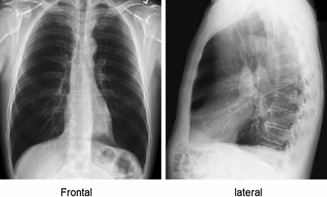
Chest X-ray view

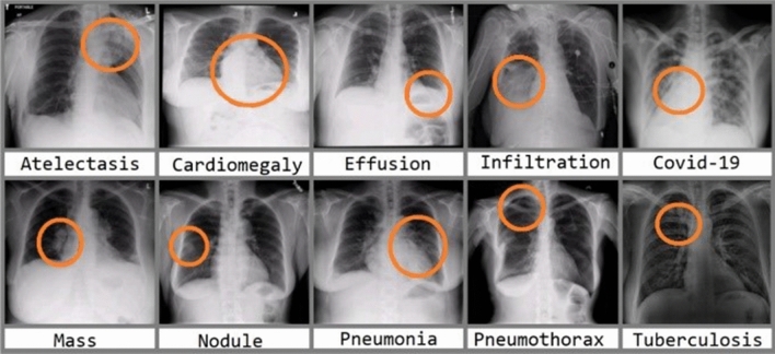
A CXR image will help doctors diagnose various diseases in the respiratory system. There are multiple diseases doctors can detect by analyzing CXR images, including COVID-19 and pneumonia [24, 25]. Figure 2 shows multiple diseases doctors may diagnose in the respiratory system.

Fig. 2.

Different types of diseases in CXR

Science is perpetually in progression, and the medical field of evaluation of CXR patients is no exception. However, errors may occur during CXR screening [19]. Some of the medical institutions in countries with limited resources and high population density do not have the necessary or up-to-date equipment to perform CXR screening.

As is often the case, the earlier TB is detected, the more effective the treatment, reducing the risk of infection. However, in some instances, patients may have to wait longer for testing, extending the spread of the infection. Active TB, distinguished by the consolidation of cavitary lesions in the lungs, has a strong likelihood of viral dissemination. TB can, however, be cured. In the respiratory system, TB is life-threatening. The danger of TB is that it can be easily transmitted to people [5, 7]. Usually, doctors study and analyze a specific area in a patient’s CXR to diagnose TB. CXR images can be segmented, analyzed, and filtered using a computer with image processing functions to improve diagnosis performance by allowing a neural network (NN) to predict the presence of TB [9].

Computer systems have witnessed significant changes over the last two decades for both broad memory space hardware and software in a variety of valuable algorithms that enable clinicians to validate and verify the diagnosis of patients [34, 35]. Methodologically, TB detection is approached by segmenting a CXR image into lung regions using deep learning (DL), specifically convolutional NNs (CNNs), along with some image processing techniques and algorithms at later stages [3, 23]. Despite the efforts made thus far, the study topic is still in its infancy and there is room for more improvement. One of the major aspects of medical diagnostic systems is to provide explainability. A system may only provide a decision, such as a positive or negative TB diagnosis; however, a medical doctor needs more than just a decision. An explainable artificial intelligence (XAI)-based system can provide visualization cues to doctors to assist in making correct decisions.

Several important contributions were reported in this study. The purpose of the proposed work is to develop a novel automatic TB detection system from CXR images using segmentation and DL models to improve the performance across different types of objective and subjective metrics to demonstrate TB detection outcomes. The proposed system will automatically predict the outcome of TB as either positive or negative based on a patient’s CXR. The performance of the system is evaluated on multiple public datasets with both positive and negative TB cases. We also used augmentation rotation in nine different angles in both normal and segmented CXR images. In addition, the proposed system incorporates XAI to visualize prediction outputs to aid medical personnel in TB diagnosis.

The following sections make up the remainder of the paper: Sect. 2 summarizes several pretrained CNN models for image classification, the original U-Net model for lung segmentation, and visualization metrics. Section 3 describes the datasets used in the experiments, augmentation steps, and methodology of the proposed study. Section 4 provides classification results for raw CXR images, segmented lung images, and each type of image with and without augmentation. The section also provides a comparison of performance between the proposed system and recent systems. Finally, Sect. 5 concludes the study and presents future work.

Background

Artificial intelligence (AI) aims to improve the ability of machines to act and behave as humans routinely while outperforming humans in image analysis and video processing [5, 36, 39]. A CNN is a DL algorithm that accepts an image as an input and learns the image from various aspects based on CNN properties [34]. The mechanism of CNN is identical to the connectivity pattern of neurons in the human brain and was inspired by the organization of the visual cortex. The human brain has approximately 86 billion neurons [32]. Neurons respond to actions in the receptive field, a restricted region of the visual field. Thus, millions of neuron interactions are required to cover the entire visual area. A computer-aided design (CAD) system with hardware and software properties is required to effectively use AI [8].

For machines to learn, software, including learning methods and multiple algorithms, must be applied. NNs accept data as input. The ability to use both AI and CAD systems opens up new avenues for researchers to develop models, and NNs can detect the target of learning machines [17, 20]. The use and analysis of multimedia data and Big Data in the medical field will yield practical results in a variety of ways, including providing a second option to doctors’ decisions and strengthening their decision for diagnosing patients. It is also quicker and less expensive to obtain these results.

CNN-based transfer learning

Authors in [27] aim to recover a degradation problem using a proposed deep residual learning framework. Mathematically, the authors denoted mapping as H(x), and F(x): = H(x) − x if nonlinear layers fit another mapping and the original mapping is recast into F(x) + x. They hypothesize that the residual should be pushed to zero if and only if a model identity mapping was optimal using a stack of nonlinear layers. This step makes it easier to optimize the residual mapping.

They also proposed the formulation of F(x) + x that can be used feedforward layers at each epoch. In addition, the authors created a shortcut connection instead of freezing some layers. The reason behind this is to establish a shortcut to simply perform identity mapping, and their outputs are added to the outputs of the stacked layers. The entire network can still be trained with backpropagation. Authors in [27] conducted comprehensive experiments on ImageNet. The goal of their effort is to show the model’s degradation problem and evaluate their proposed architecture. They also compared two models, which are 18-layer and 34-layer residual nets (ResNets). Input images are resized, cropped, augmented, and resampled. The 34-layer plain net has a higher training error throughout the training procedure even though the solution space of the 18-layer plain network is a subspace of that of the 34-layer plain network. The reverse occurs with residual learning—in this case, the 34-layer ResNet is better than the 18-layer ResNet (by 2.8%). More importantly, the 34-layer ResNet exhibits considerably lower training error and is generalizable to validation data [27]. The authors also considered both “Top-1-err” and “Top-5-err” terms to evaluate the proposed architecture. The top-1 error represents the ratio of time that the classifier (ResNet) did not give the correct class. The top-5 error represents the ratio of time that the classifier did not involve the correct class among the top five probabilities. ResNet scored the lowest number in Top-1-error and Top-5-error with 21.43 and 5.71%, respectively.

Authors in [28] began with some speculative principles, and it will be necessary to assess the principles’ accuracy and domain of validity. Network architectures are being improved by detecting deviations and correcting results. There are four main principles, starting with input data representation size and decreasing successively from inputs to outputs until the final representation is reached. In image classification, higher-dimensional representation facilitates local processing while training a network. To allow for more disentangled features, activations in CNNs must be increased. Spatial aggregation can be performed over a lower-dimensional embedding with little or no loss in representational power. The width and depth of the network are balanced. The optimal performance of the network can be reached by balancing the number of filters per stage and the depth of the network.

Authors in [29] proposed a CNN architecture with a unique ability, which is its architecture can separate convolution layers depth-wise. The authors hypothesized that mapping plays the main role. The hypothesis is that both mappings of cross-channel correlations and spatial correlations in the feature maps of CNNs can be entirely decoupled. Their proposed architecture was known as “Extreme Inception,” i.e., Xception [29].

The Xception architecture base contains 36 convolutional layers for feature extraction. In [29], the experiment was solely focused on image classification. In short, the Xception architecture is a linear stack of depth-wise separable convolution layers with residual connections. The Xception architecture routes data through the entry flow, which has an image size of 299 × 299; then the middle flow, which is repeated eight times; and finally the exit flow. Note that all convolution and separable convolution layers are followed by batch normalization (not included in the diagram). All separable convolution layers use a depth multiplier of 1 (no depth expansion). The Xception architecture scored better results with a Top-1 accuracy of 79% and Top-5 accuracy of 94.5%.

In recent literature, there has been a growing interest in developing small and efficient neural networks. Recently, there has been rising interest in building small and efficient neural networks in recent literature. Authors in [30] proposed network architecture with different capabilities that enable the use of a model with restrictions in latency and size. Specifically, MobileNet prioritizes latency to optimize with balancing with network size. In addition, the authors cited multiple approaches for obtaining small networks based on pertained networks such as Xception and Squeezenet. The authors consider the base of the architecture is depth-wise convolution and a 1 × 1 convolution, also known as point-wise convolution. Point-wise convolution can use a single filter in each input channel. In comparison, a standard convolution can use both filters and combine inputs into a new set of outputs in a single step. During training, the authors considered that all point-wise layers are followed by batch normalization with a nonlinear activation function (a rectified linear unit, ReLU), except for the final fully connected layer, which has linear activation and feeds into a SoftMax layer for classification.

Recently, Tan et al. [31] defined an efficient way to design CNN models by exploring the relationship between the width and depth of CNN models. The authors aimed to design CNN models with fewer parameters while providing better classification accuracy. The name of these CNN models is derived from the technique, and they are known as EfficientNet CNN models. In their original paper, the authors proposed seven such models, which they named EfficientNetB0 to EfficientNetB7. When used on the ImageNet dataset, the EfficientNet CNN models outperformed all other models in terms of parameter number and Top-1 accuracy.

Another idea is to include an attention module at lower convolutional layers because higher layers’ features represent large receptive fields with highly overlapping regions, which means that the attention mechanism may not be effective with these features. We propose that we investigate other options. In other words, the attention branch has now been added to intermediate blocks of the model, giving the model two separate branches. This also means that the model has two outputs that must be optimized jointly.

U-Net

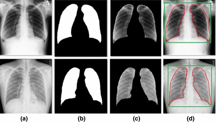
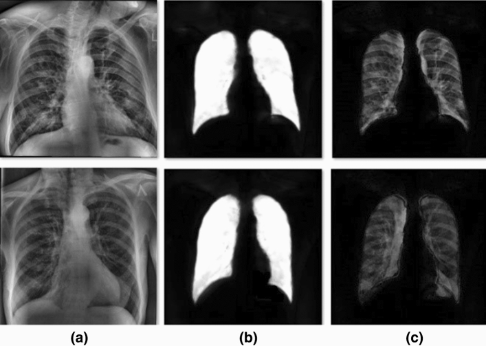
U-Net is a CNN architecture that expands with a clear goal: learning how to detect the desired objects in tested images from a series of images. U-Net is an architecture for semantic segmentation. The name is derived from the algorithm's network architecture, which resembles the letter U. The main purpose of U-Net is to achieve medical image segmentation [8]. Figure 3 shows the result of the U-net algorithm in steps.

Fig. 3.

Steps for lung segmentation: a original image, b lung mask, c output segmentation, and d segmented region of interest

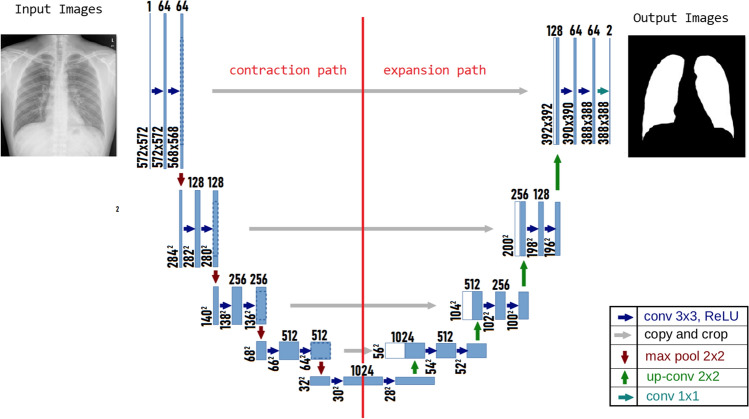
Input images are added to a constructing path. The constructing path is used to extract and detect relevant factors in the input images. Therefore, in this path, there is a stack of convolutional and max-pooling layers. This path consists of 3 × 3 convolutions followed by ReLU and a 2 × 2 max-pooling operation with stride two for downsampling; this process is repeated. The number of channels must be doubled for each downsampling of the images; otherwise, important information might be lost. Another path is the expansion path, which is used to enable precise localization using transposed convolutions. Figure 4 explains the paths and U-Net architecture with colored arrows pointing to the operation. This path consists of an upsampling of the feature map followed by a 2 × 2 convolution, which is the opposite of the first path in that it halves the number of feature channels, a concatenation with the correspondingly cropped feature map from the contracting path, and 3 × 3 convolutions followed by a ReLU twice. The cropping is necessary to prevent the loss of border pixels in every convolution. In total, U-Net has 23 layers, including the final layer, and a 1 × 1 convolutional is used to map each 64-component feature vector to the desired number of classes [26].

Fig. 4.

U-Net architecture

Visualization metrics

t-SNE is an abbreviation for t-distributed stochastic neighbor embedding. It is a nonlinear unsupervised approach used for data exploration and high-dimensional data visualization. A unique benefit is a nonlinear technique that allows imaging several structures using this utility. t-SNE is a dimensionality reduction machine learning (ML) technique that helps classify related trends. In t-SNE, patterns in a high-dimensional dataset are represented as points close to each other, and they will be displayed as being close to each other in a chart, resulting in a visually appealing visualization.

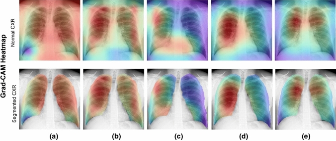
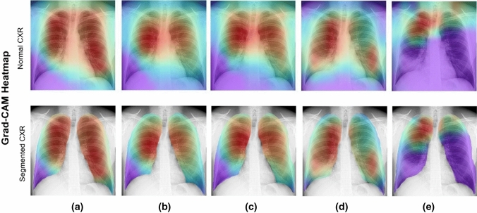
Gradient-weighted class activation mapping (Grad-CAM) uses the gradients of any target concept, in this case, lung TB detection, to generate a coarse localization map highlighting important regions to predict TB in CXR. The findings will aid doctors’ decision-making process.

Methodology

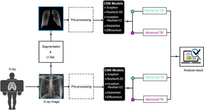
During our experiment, we study and analyze different DL methods for TB detection in a patient's radiography. We propose an automatic TB detection system for CXR images in the thesis. We study the system by incorporating the above observations. The system uses segmented lung CXR images and recent pretrained CNN models. It is evaluated on multiple datasets and cross-dataset scenarios. The system includes several blocks, and each block will be described below. Each block depends on the previous one, and the proposed model can be considered a consequential system. Figure 5 shows a block diagram of the proposed TB detection system. Each block in the figure corresponds to one main stage of the proposed system.

Fig. 5.

Block diagram of the proposed TB detection system

In this work, we aim to design an automatic TB detection system for CXR images using DL models. More specifically, we investigate some recent CNN models used for detection. To achieve our objectives, the research methodology involves the following steps:

• System design

• Dataset preparation

• Convenient CNN

• Comparison with different systems using several performance metrics

In our research, we propose an automatic TB detection system using DL tools and ML techniques to achieve our goal. The proposed system has three main elements, which begin with a patient’s CXRs taken by a radiographer. Input CXR images come from multiple publicly available datasets, enabling researchers to conduct their experiments and achieve their objectives as well as use them for research and development of CAD systems. Generally, image datasets are used in the medical field for detecting TB. Normally, input images need to be enhanced using image processing techniques in subsequent stages to minimize error rates and boost detection performance, which is the main aim of our proposed system. Optionally, some filters may be used to enhance the edges of an image. Filters will also help in extracting spatial and temporal features in an image. In this sense, a more thorough exploratory data analysis and preprocessing, with lung group filtering for people of various ages, genders, and geographical origins, will be promising [20]. The outputs of the preprocessing block are enhanced images or updated image input. After the features for the next block are extracted, these images are ready and convenient.

Both publicly available datasets Montgomery and Shenzhen include masks of the lung in CXRs. The nature of the mask is simple, which includes only two colors: black and white. After multiplying the images by their respective mask, only lung images are obtained, which we call segmented images [4, 5]. Lung field segmentation is an essential preprocessing step to extract the region of interest (ROI) from input CXR images [15]. Several segmentation approaches have recently been proposed to obtain segmented images. However, the segmentation procedures of different approaches such as active appearance models and a multi-resolution pixel classification method differ [19]. The segmentation was applied before in many other types of medical images [37, 38].

We split input datasets into two parts. The first part is extracting the ROI in both datasets (Montgomery and Shenzhen). Therefore, both datasets contain a mask of the lung area from which we can detect TB. The two datasets provide ROI masks (left and right). Typically, ROI procedures are used in medical imaging. The explanation for extracting the ROI in medical images is that we want to concentrate more on the region where TB occurs in CXR images. A significant area of a typical CXR image contains black pixels, which have no contribution to the detection of TB. Therefore, using an entire CXR image may result in confusing features. Concentrating on the ROI will also speed up computation. The ROI extraction formula is

$${\text{ROI}}_{\left(x,y\right)}={\text{Input Image}}_{\left(x,y\right)}.{\text{ShaddingImage}}_{\left(x,y\right).}$$ 1

In the above equation, each pixel (x,y) value of an input image is multiplied by the corresponding mask (shaded) pixel value (either 0 or 1).

After segmentation, in the third stage, a CNN model will use both original datasets images and segmented images to extract deep learned features and classify the images. In addition, we will apply augmentation rotation to both the original and segmented images and compare their results. We also will compare our results with those of other researchers. We adopt a fivefold cross-validation approach, where the whole dataset was divided into five equal groups, and in each run, four of them were used in training and the remaining was used in testing. After five runs, all the groups were tested. Several pretrained CNN models are available in the literature. However, we will investigate the following five CNN models because they are comparatively newer and more efficient:

• Xception (2016)

• Inception-ResNet-V2 (2016)

• ResNeXt-50 (2017)

• MobileNet (2017)

• EfficientNet (2019)

Dataset

In our experiment, the collected datasets are publicly available from the National Library of Medicine for TB. Table 1 presents all features of datasets used in our experiment; the datasets are as follows:

• Montgomery

• Shenzhen

• Belarus

Table 1.

Dataset information

Information	Montgomery	Shenzhen	Belarus
Active cases	58	336	304
Inactive cases	80	326	None
Total cases	138	662	304
Cross-validation subset	27, 28	132, 133	Null
Men (%)	44.2	66.4	47.9
Women (%)	31.4	21	32
Children (%)	24.4	12.6	20.1
File type	PNG	PNG	PNG
Bit depth	8-bit	8-bit	8-bit
CR/DR	CR	DR	CR + DR
Resolution	4020 × 4892	948–3001 × 1130–3001	512 × 512
Image view	Frontal view	Frontal view	Frontal view
Image type	Grayscale	Grayscale	Grayscale

Montgomery County X-ray Dataset: X-ray images in this dataset have been collected from the TB control program of the Department of Health and Human Services of Montgomery County, MD, USA [3, 6].

Shenzhen Hospital X-ray Dataset: X-ray images in this dataset have been collected from Shenzhen No. 3 Hospital in Shenzhen, Guangdong province, China. The X-rays were acquired as part of the routine care at Shenzhen Hospital [3, 6].

Belarus X-ray Dataset: X-ray images in this dataset have been collected from the institutional review board at Thomas Jefferson University Hospital. Belarus Tuberculosis Portal maintained by the Belarus TB public health program [3].

Both the Montgomery and Shenzhen datasets contain both active and inactive TB cases. The Belarus dataset contains only active TB cases. Images can be categorized into two types, which are digital radiography (DR) and computed radiography (CR). Both types can be switched using conversion methods through software. In the Belarus dataset, some images (six samples) are negated because they do not contain the ROI, especially the lung or CXR, and were taken in lateral view, which does not allow for detecting TB. The total number of images in the Belarus dataset used in the experiment is 298. Figure 6 illustrates the negated images from the Belarus dataset.

Fig. 6.

Image negated from Belarus dataset

In the experiment, we will study the Montgomery and Shenzhen datasets separately because they have both TB cases. Then, we will study the combination of the three datasets. Figure 7 shows the total number of samples in the combination of the datasets. The number of TB samples is the addition of all TB samples in three datasets minus the six specific cases in the Belarus dataset mentioned before. The number of no TB samples is the addition of all no TB samples in the Montgomery and Shenzhen datasets, because there are no such cases in the Belarus dataset. Then we adopt the fivefold cross-validation approach. The experiments using the combined dataset will testify the robustness of the system irrespective of images taken at a particular setup.

Fig. 7.

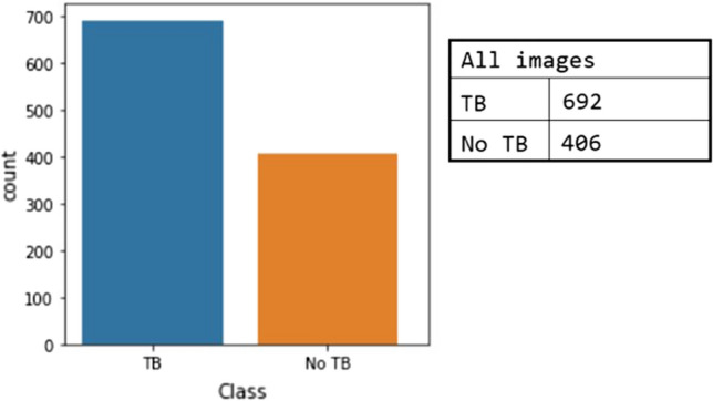
Data distribution in combined dataset experiments for normal and segmented CXR images

Augmentation rotation

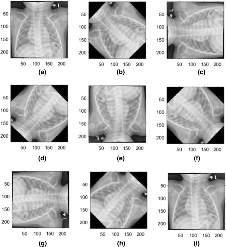
The performance of DL NNs depends on the amount of available data, resulting in the need for a large amount of data to improve DL models’ learning performance. Data augmentation is a technique to artificially create new training data from existing training data. Typically, using a data augmentation technique during model training increases the training time. During the training stage, image data augmentation can be used to create transformed versions of a single image with the original image's features. The transformed image differs from the original image in that it has been shifted, rotated, or zoomed. Next, we will rotate training images clockwise by a specified number of degrees ranging from 0 to 360. The degrees will be incremented by 45°. As a result, a single image in the training stage will be rotated at nine different angles. We adopt the rotation augmentation because the interpretation of CXR images does not change with the rotation. Figure 8 shows examples of a single CXR image that has been rotated in nine different angles.

Fig. 8.

CXR images after augmentation using nine different angles: a 0°, b 45°, c 90°, d 135°, e 180°, f 225°, g 270°, h 315°, and i 360°

CNN processing

Image normalization should be performed before training and evaluating DL models. Reducing the dimension of input images is an initial step in ML. CNN models for classification applications have specific image sizes. Thus, the models first use the input image size and then adjust to the various sizes of convolutional layers; several mathematical formulas and techniques are used in this process. Table 2 illustrates the sizes of each CNN model in our experiment.

Table 2.

CNN models’ general information

CNN model	Xception	ResNeXt-50	Inception-ResNet-V2	MobileNet	EfficientNetB3
Input size	299 × 299	224 × 224	224 × 224	224 × 224	224 × 224
Parameters	22.9 Million	25.6 Million	55.8 Million	4.2 Million	12.3 Million
Year published	2017	2015	2015	2017	2019
Size (MB)	88	96	215	16	48
Depth	126	–	527	88	–
Layers number	71	50	164	28	327

Experiment

In principle, transfer learning refers to the use of learned knowledge from a previous event in a domain, such as training a model, to train another model in a related domain [2].

Recent studies [2, 3, 22, 23] have demonstrated that using a pretrained model on the ImageNet dataset and then fine-tuning with more specific datasets yield outstanding classification and detection results. The purpose of using a pretrained model is to enable the five CNN models to improve their generalization ability for natural images [2]. During the experiment, we use the Adam optimizer [33] with a learning rate of 1-e4, mini-batch size of 32 images, dropout rate = 0.2, and 200 epochs. We also used a Windows® system with Intel® Xeon® CPU E5-2640v3 3.00-GHz processor, 2 TB of hard disk space, 16-GB RAM, and a CUDA-enabled NVIDIA GTX 1080 Ti 11-GB graphical processing unit. The networks were implemented using TensorFlow and Keras libraries in Python 3.8.5. Instead of starting with random weight values during the training of the five CNN models, convergence is achieved after at least 20 epochs with a batch size of 32 images as a default value. In addition, all images in the experiments are CXR in frontal view PA, as previously mentioned, and we used a cross-validation technique in the experiment.

Results and discussions

Performance metrics

Evaluating a system is an essential part of an experiment, and it includes several measurements used to evaluate the final system’s performance in terms of its expected goals and to assess its future applicability. Performance evaluation metrics can be objective result which is describing the system as number as accuracy and precision. The subjective result is describing the system as a graph which can be evaluated by visualization perception. The following metrics are used in this study:

• Accuracy

• Recall

• Precision

• F1-score

• Kappa value

• Confusion matrix

The following additional visualization metrics can provide an assessment and illustration:

• Model Accuracy vs. epoch

• Model Loss vs. epoch

• The area under the curve (AUC)-receiver operating characteristics (ROC)

• t-SNE

• grad-CAM

The most powerful and widely used metric for model evaluation is the proportion of the overall number of accurate predictions. Accuracy is essential in ML for measuring the classification performance of an algorithm. Accuracy is the percentage of images correctly predicted of all input images. Accuracy can be calculated as

$$\text{Accuracy}=\left(\frac{\sum \text{Correct prediction}}{\sum \text{Input samples}}\right)$$ 2

Recall is the measure of how accurately a model can distinguish common data features; it is the proportion of actual positive cases that are reported correctly. Recall can be calculated as

$$\text{Recall}=\left(\frac{\sum \text{Only positive cases prediction}}{\sum \text{Input samples}}\right)$$ 3

Precision is the measure of the relevant data images. It is salient that doctors do not administer TB medications to patients without TB, whereas a TB detection model predicted a positive TB case for such patients. Precision is the ratio between true predicted positive cases and all predicted positive cases or the number of items classified correctly as positive out of the total items recognized as positive. The formula is

$$\text{Precision}=\left(\frac{\sum \text{Identify positive}}{\sum \text{Identified positive}}\right)$$ 4

F1-score conveys the balance between precision and recall. The present authors aim to achieve the highest accuracy and recall simultaneously in certain situations. The harmonic mean for accuracy and recall values is F1-score. The formula is

$$F1={\left(\frac{{\text{Recall}}^{-1}+{\text{Precision}}^{-1}}{2}\right)}^{-1}$$ 5

Kappa value statistics are an essential metric that can effectively manage multi-class and imbalanced class issues. The formula is

$$Kappavalue=\left(\frac{{\mathcal{P}}_0-{\mathcal{P}}_e}{1-{\mathcal{P}}_e}\right)=\left(1-\frac{1-{\mathcal{P}}_0}{1-{\mathcal{P}}_e}\right)$$ 6

where ${\mathcal{P}}_e$ represents the expected value of correct prediction and ${\mathcal{P}}_0$ the observed value of prediction.

A confusion matrix is a table to describe the performance of a classification model on a set of test data. Based on the number of classes in the experiment, the table will be separated. A confusion matrix provides useful information about a model, and it can be easily understood because its result representation is simple.

The main task of accuracy is to determine whether a model is best at identifying relationships and patterns between variables in a dataset based on an input. It is the relation between training and test accuracy in the Y-axis, and in the X-axis, it is the number of epochs to illustrate changes in accuracy per epoch.

One of the most visual performances used in ML is the AUC ROC curve, and it is one of the most important evaluation metrics for evaluating the performance of a classification model. Fundamentally, ROC is a probability curve, and AUC represents the degree or measure of separability. A ROC curve is a graph showing at all classification thresholds the output of a classification model. Comprehensively, ROC-AUC shows the ability of a trained model at distinguishing between classes. The higher the AUC, the better the trained model’s predictability.

The higher the AUC, the better the model is at distinguishing between patients with normal or abnormal TB. The ROC curve plots a graph that contains the relationship between the false positive rate (FPR) on the X-axis and the true positive rate (TPR) on the Y-axis.

Results

This state-of-the-art performance of our proposed system was compared with the recently published efforts toward the same goal. Table 3 summarizes the comparison of this study’s results to those of other studies for detecting TB from CXR images. Some of these efforts used publicly available datasets, such as [9, 12], whereas others used private datasets, such as [8, 11].

Table 3.

Comparison with other recent similar works

Work	Year	Images	Dataset	Method	Results
Lakhani et al. [1]	2017	1007	-Montgomery -Shenzhen -Belarus	Two CNN models using normal CXRs. Used augmentation compression	AUC is 98%
Becker et al. [8]	2017	–	Mulago National Hospital	Detecting patterns in photographs	Accuracy of 98%
Liu et al. [5]	2017	4248	Partners in Health Peru	CNN transfer learning	Accuracy of 85.68%
Antani et al. [22]	2018	1920	-Kenya -India	Six CNN pretrained models	Accuracy 95.6%
Stirenko et al. [6]	2018	800	-Montgomery -Shenzhen	CNN segmented lung CXRs	Accuracy lower than 85%
Hwang et al. [11]	2019	4559	Seoul National Hospital	Develop deep learning	AUC is 97.1%
Nguyen et al. [9]	2019	1032	-Montgomery -Shenzhen	Five CNN models using transfer learning	AUC is 99%
Heo et al. [12]	2019	800	-Montgomery -Shenzhen	Five CNN pretrained models	AUC is 92.13%
Rahman et al. [23]	2020	7000	Montgomery Shenzhen Belarus Health NIAID TB dataset	Nine CNN using normal and segmented lung CXRs	Accuracy of 96.5% for normal CXR. Accuracy of 98.6 for segmented CXRs
This study	2021	1098	-Montgomery -Shenzhen -Belarus	Segmented and augmented lung CXRs	For combined dataset: AUC = 0.999; average accuracy = 98.7%, using EfficientNetB3

Figure 9 shows the results of U-Net samples and steps for segmenting lung images. Table 4 provides the main information of the experiments using the U-Net.

Fig. 9.

U-Net output segmentation results for two sample lung CXR images. a shows the original images. b shows the results of U-Net. c show the results after ROI extraction

Table 4.

U-Net main information in experiments

#	Method	Information
1	Training images	704 original images 704 mask images
2	Test images	394 images
3	Input Image size	512 × 512
4	Optimizer	Adam
5	Learning rate	0.0001
6	Epochs per step	300
7	Epochs	5
8	Training time	09:24:12
9	Testing time	00:18:12
10	Training accuracy	0.942
11	Loss	0.1439
12	Total params	31,057,985
13	Trainable params	31,044,289
14	Non-trainable params	13,696

Figure 10 shows the training and validation loss versus epochs for the five CNN models for augmented segmented lung CXR images. From this figure, we see that for ResNet50 and EfficientNetB3, the loss graphs are smooth, and the system are nicely converging.

Fig. 10.

Model loss for augmented segmented CXR images

The ROC curve of TB disease detection in the cohorts demonstrates the excellent ability of the proposed system to localize abnormal areas in the CXR. The FPR, also known as specificity, is on the X-axis, and the TPR, also known as sensitivity, is on the Y-axis. Figure 11 shows the performance of the five CNN models using the augmented segmented CXR images of the combined dataset.

Fig. 11.

Comparison between five CNN models using ROC-AUC

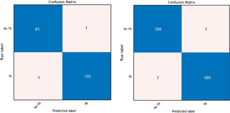
Owing to the importance of a confusion matrix, we will show the performance of EfficientNetB3 using a confusion matrix in Fig. 12. As mentioned earlier, there are four different experiments:

1. Normal CXR images

2. Segmented CXR images

3. Normal CXR images with augmentation

4. Segmented CXR images with augmentation

Fig. 12.

Confusion matrix for efficientNetB3 for segmented augmented CXR images in the combined dataset. Left: a confusion matrix for the best accuracy using cross-validation; right: a confusion matrix using average rounds

These are applied first to the Montgomery dataset, then to the Shenzhen dataset, and, finally, to all three datasets for the classification of abnormal active TB and normal no TB cases. Table 5 displays the average results for both normal and segmented CXR images without augmentation. Table 6 illustrates the average results for both normal and segmented CXR images with augmentation. Furthermore, Table 7 displays the best results for both normal and segmented CXR images without augmentation. Finally, Table 8 shows the best results for both normal and segmented CXR images with augmentation.

Table 5.

Comparative average rounds of cross-validation results of five CNN models for TB detection in the combined dataset without augmentation in nine angles

Schema	Dataset	CNN models	Average weighted
			Accuracy (%)	Recall (%)	Precision (%)	F1-Score (%)	Specificity (%)	Kappa value (%)
Without Segmentation Without Augmentation	Montgomery dataset	ResNet50	68.7	73.1	71.3	72.3	61.7	34.9
		Xception	73.9	77.5	77.5	77.5	69.0	46.5
		InceptionRenNetV2	77.5	78.2	85.0	81.4	76.5	53.1
		MobileNet	68.9	73.4	72.5	73.0	62.7	36.2
		EfficientNetB3	82.80	83.3	87.5	85.4	81.5	64.0
	Shenzhen dataset	ResNet50	77.0	76.7	76.7	76.7	77.4	54.1
		Xception	80.1	81.7	76.7	79.1	78.7	60.1
		InceptionRenNetV2	83.8	85.2	81.3	83.2	82.6	67.6
		MobileNet	79.3	79.4	78.2	78.8	79.2	58.6
		EfficientNetB3	87.6	89.4	85.0	87.1	86.1	75.2
	Combination dataset	ResNet50	88.7	82.8	87.8	85.2	92.6	76.1
		Xception	87.4	79.6	88.7	83.9	92.9	73.7
		InceptionRenNetV2	90.6	84.7	91.1	87.8	94.6	80.2
		MobileNet	88.6	81.3	89.9	85.4	93.7	76.1
		EfficientNetB3	90.3	84.5	90.1	87.2	94.0	79.4
With Segmentation Without Augmentation	Montgomery dataset	ResNet50	73.2	77.2	76.3	76.7	67.8	45.1
		Xception	77.0	79.3	81.2	73.2	73.2	52.2
		InceptionRenNetV2	81.2	83.8	83.8	83.8	77.6	61.3
		MobileNet	72.5	76.9	75.0	75.9	66.7	43.8
		EfficientNetB3	85.5	88.5	86.3	87.3	81.7	70.4
	Shenzhen dataset	ResNet50	84.7	86.6	81.6	84.0	83.1	69.5
		Xception	86.1	88.0	85.5	84.5	84.5	72.2
		InceptionRenNetV2	89.6	90.8	87.7	89.2	88.5	79.1
		MobileNet	86.3	88.3	83.1	85.6	84.5	72.5
		EfficientNetB3	90.3	91.7	88.3	90.0	89.1	80.6
	Combination dataset	ResNet50	88.5	84.3	84.7	84.5	91.0	74.4
		Xception	89.9	86.1	86.7	86.4	91.2	78.3
		InceptionRenNetV2	90.8	87.5	87.8	87.5	92.8	80.4
		MobileNet	90.7	86.9	88.2	87.5	93.0	80.1
		EfficientNetB3	91.2	87.4	88.9	88.2	93.4	81.1

The best result of each set has been bolded

Table 6.

Comparative average rounds of cross-validation results of five CNN models for TB detection in the combined dataset with augmentation in nine angles

Schema	Dataset	CNN models	Average weighted
			Accuracy (%)	Recall (%)	Precision (%)	F1-Score (%)	Specificity (%)	Kappa value (%)
Without Segmentation With Augmentation	Montgomery dataset	ResNet50	72.5	76.9	75.0	75.9	66.7	43.8
		Xception	76.8	81.6	77.5	79.5	71.0	52.9
		InceptionRenNetV2	84.1	85.4	87.5	86.4	82.1	67.1
		MobileNet	76.1	78.3	81.3	79.8	72.7	50.6
		EfficientNetB3	85.5	85.7	90.0	87.8	85. 2	70.0
	Shenzhen dataset	ResNet50	83.2	82.7	83.3	83.1	83.8	66.5
		Xception	83.8	83.1	84.4	83.7	84.6	67.7
		InceptionRenNetV2	90.6	91.8	89.0	90.3	89.6	81.3
		MobileNet	84.3	83.8	84.4	84.1	84.7	68.6
		EfficientNetB3	92.6	93.4	91.4	92.4	91.8	85.2
	Combination dataset	ResNet50	90.8	88.2	86.7	87.5	92.3	80.2
		Xception	89.7	85.0	87.7	86.3	92.6	78.1
		InceptionRenNetV2	91.7	87.6	90.4	89.0	94.3	82.3
		MobileNet	90.6	85.6	89.7	87.6	93.8	80.1
		EfficientNetB3	91.1	86.7	89.7	88.1	93.8	81.0
With Segmentation With Augmentation	Montgomery dataset	ResNet50	80.4	84.4	81.3	82.8	75.4	60.1
		Xception	84.8	88.3	85.0	86.6	80.0	69.0
		InceptionRenNetV2	85.5	87.5	87.5	87.5	82.8	70.3
		MobileNet	82.6	85.0	85.0	85.0	79.3	64.3
		EfficientNetB3	89.9	89.3	93.8	91.5	90.7	79.0
	Shenzhen dataset	ResNet50	90.0	89.5	89.2	89.4	89.6	79.1
		Xception	90.3	91.7	88.3	90.0	89.1	81.7
		InceptionRenNetV2	93.7	93.6	93.6	93.6	93.8	87.3
		MobileNet	90.6	90.5	90.5	90.5	90.8	81.5
		EfficientNetB3	93.7	93.6	93.6	93.6	93.8	87.3
	Combination dataset	ResNet50	91.3	90.8	85.2	87.9	91.6	81.2
		Xception	93.7	94.2	88.4	91.2	92.4	86.3
		InceptionRenNetV2	98.1	98.7	96.1	97.1	97.7	95.9
		MobileNet	95.3	94.9	92.1	93.5	95.5	89.8
		EfficientNetB3	98.7	98.3	98.3	98.3	99.0	97.2

The best result of each set has been bolded

Table 7.

Comparative best round of cross-validation results of five CNN models for TB detection in the combined dataset without augmentation in nine angles

Schema	Dataset	CNN models	Best weighted						ROC-AUC
			Accuracy (%)	Recall (%)	Precision (%)	F1-Score (%)	Specificity (%)	Kappa value (%)
Without Segmentation Without Augmentation	Montgomery dataset	ResNet50	71.4	78.6	68.8	73.3	64.3	42.2	77.6
		Xception	77.8	85.7	75.0	80.0	69.2	55.2	85.4
		InceptionRenNetV2	85.7	92.9	81.3	86.7	78.6	71.4	89.6
		MobileNet	75.0	84.6	68.8	75.9	66.7	50.5	81.8
		EfficientNetB3	89.3	93.3	87.5	90.3	84.6	78.4	92.0
	Shenzhen dataset	ResNet50	79.5	82.7	73.8	78.1	77.0	59.0	89.8
		Xception	84.1	83.3	84.6	84.0	84.8	68.2	90.6
		InceptionRenNetV2	87.9	87.7	87.7	87.7	88.1	75.8	91.4
		MobileNet	80.0	82.0	75.8	78.7	78.1	59.6	90.3
		EfficientNetB3	89.4	89.2	89.2	89.2	89.6	78.9	92.7
	Combination dataset	ResNet50	88.7	82.8	87.8	85.2	92.6	76.1	93.3
		Xception	87.7	80.0	88.9	84.2	93.1	74.2	91.5
		InceptionRenNetV2	92.3	91.1	87.8	89.4	93.0	83.4	95.4
		MobileNet	88.6	82.6	87.7	85.0	92.5	75.9	93.9
		EfficientNetB3	90.5	86.5	87.8	87.3	92.8	79.7	94.9
With Segmentation Without Augmentation	Montgomery dataset	ResNet50	75.0	80.0	75.0	77.4	69.2	49.5	82.3
		Xception	82.1	82.0	82.0	82.0	76.9	64.0	89.6
		InceptionRenNetV2	85.7	92.9	81.3	86.7	78.6	71.4	92.2
		MobileNet	75.0	84.6	75.8	74.0	66.7	50.5	84.9
		EfficientNetB3	88.9	93.3	87.5	90.3	83.3	77.3	92.7
	Shenzhen dataset	ResNet50	86.6	86.4	86.4	86.4	86.4	73.1	90.6
		Xception	86.4	87.5	84.8	86.2	85.2	72.7	90.0
		InceptionRenNetV2	91.0	92.2	89.3	90.7	90.0	82.1	96.3
		MobileNet	88.8	88.1	89.4	88.7	89.6	77.6	88.8
		EfficientNetB3	92.4	92.3	92.3	92.3	92.5	84.8	98.0
	Combination dataset	ResNet50	89.6	87.3	84.1	85.7	90.9	77.6	95.4
		Xception	90.0	86.4	86.4	86.4	92.1	78.5	96.9
		InceptionRenNetV2	91.8	88.9	88.9	88.9	93.5	82.4	98.3
		MobileNet	91.4	90.8	85.2	87.9	91.7	81.2	99.0
		EfficientNetB3	93.6	92.4	90.1	91.3	94.3	86.3	99.4

The best result of each set has been bolded

Table 8.

Comparative best round of cross-validation results of five CNN models for TB detection in the combined dataset with augmentation in nine angles

Schema	Dataset	CNN models	Best weighted						ROC-AUC
			Accuracy (%)	Recall (%)	Precision (%)	F1-Score (%)	Specificity (%)	Kappa value (%)
Without Segmentation With Augmentation	Montgomery dataset	ResNet50	75.0	80.0	75.0	77.4	69.2	49.5	85.4
		Xception	81.1	85.7	80.0	82.8	76.9	60.8	88.1
		InceptionRenNetV2	88.9	93.3	87.5	90.3	83.3	77.3	92.7
		MobileNet	81.5	92.3	75.0	82.8	71.4	63.2	88.8
		EfficientNetB3	89.3	93.3	87.5	90.3	84.6	78.4	95.3
	Shenzhen dataset	ResNet50	84.1	84.4	83.1	83.7	83.2	68.2	89.5
		Xception	85.1	84.8	84.8	84.8	85.3	70.4	90.2
		InceptionRenNetV2	91.0	90.9	90.9	90.9	91.2	82.1	94.2
		MobileNet	85.6	84.8	86.2	85.5	86.4	71.2	92.7
		EfficientNetB3	93.9	92.5	95.4	93.9	95.4	87.9	98.0
	Combination dataset	ResNet50	92.3	90.1	89.0	89.6	93.6	83.5	99.3
		Xception	91.8	89.9	87.7	88.8	92.9	82.3	99.2
		InceptionRenNetV2	93.7	90.5	92.7	91.6	95.7	86.5	99.8
		MobileNet	92.7	90.1	90.1	90.1	94.2	84.4	99.6
		EfficientNetB3	92.7	90.1	90.1	90.1	94.2	84.4	99.8
With Segmentation With Augmentation	Montgomery dataset	ResNet50	82.1	92.3	75.0	82.8	73.3	64.6	91.7
		Xception	88.9	93.3	87.5	90.3	83.3	77.3	93.3
		InceptionRenNetV2	88.9	93.3	87.5	90.3	83.3	77.3	93.8
		MobileNet	85.1	92.9	81.3	86.7	76.9	70.2	92.2
		EfficientNetB3	92.6	93.3	93.3	93.3	91.6	85.5	95.8
	Shenzhen dataset	ResNet50	90.2	89.4	90.8.	90.1	90.9	80.3	98.3
		Xception	92.4	92.3	92.3	92.3	92.5	84.8	99.2
		InceptionRenNetV2	94.7	95.3	93.8	94.6	94.1	89.4	99.6
		MobileNet	93.3	92.5	93.9	93.2	94.0	86.6	99.5
		EfficientNetB3	96.2	96.9	95.4	96.1	95.6	92.4	99.8
	Combination dataset	ResNet50	94.1	92.5	91.4	92.0	95.0	87.3	99.5
		Xception	96.0	94.0	95.1	94.5	97.1	91.3	99.6
		InceptionRenNetV2	98.2	97.5	97.5	97.5	98.5	96.1	99.9
		MobileNet	96.8	96.3	95.1	95.7	97.1	93.1	99.8
		EfficientNetB3	99.1	98.8	98.8	98.8	99.2	98.1	99.9

Best result of each set has been bolded

According to the results in Tables 5–8, the five CNN pretrained models achieve high performance in classifying TB from normal images in this two-class problem. Notably, network performance is not dependent on network depth. RenNet50 is deeper than MobileNet, but MobileNet achieves better performance. EfficientNetB3 demonstrates a good example of transfer learning and output compared to the other networks for detecting TB.

Visualization

Visualization techniques are used to illustrate important information; the t-SNE visualization technique will confirm that NN layers can create discriminating features between both classes, TB and normal CXR images. The t-SNE technique is better in visualizing high-dimensional data into a two-dimensional map. The t-SNE technique was implemented on a Python platform, with multiple parameters as dimensions and a perplexity-effective number of neighbors [23]. The parameters were modified from default values to confirm the performance of all networks on the combined dataset; the t-SNE visualization is shown in Figs. 13–16. From these figures, we see that the TB and no TB samples are clearly separated using both the segmentation and the augmentation (Fig. 16).

Fig. 14.

t-SNE for segmented CXR images in the combined dataset

Fig. 15.

t-SNE for normal CXR images in the combined dataset after applying augmentation

Fig. 13.

t-SNE for normal CXR in the combined dataset

Fig. 16.

t-SNE for segmented CXR images in the combined dataset after applying augmentation

It is essential to observe the efficiency of training an ML model to reveal its network learning distribution in relation to the various available data. Thus, during our experiments, we demonstrate the learning performance of the five CNN models using the combined dataset, which contains a higher number of CXR images, and this is shown using grad-CAM-based heat maps generated for the following original cases:

1. Normal CXR images

2. Segmented CXR images

3. Augmentation in non-segmented CXR images

4. Augmentation in segmented CXR images

Figures 17–20 show the learning performance of all CNN models for each sample, along with their heat maps on the normal CXR images, segmented CXR images, augmented normal CXR images, and augmented segmented CXR images. From these figures, we see that the presence of TB is more correctly visualized in the segmented and augmented images (Fig. 20).

Fig. 18.

Grad-CAM visualization of classified TB in raw CXR images with augmentation without segmentation: a ResNet50; b Xception; c MobileNet; d InceptionResNetV2; and e EfficientNetB3

Fig. 19.

Grad-CAM visualization of classified TB in segmented CXR images without augmentation: a ResNet50; b Xception; c MobileNet; d InceptionResNetV2; and e EfficientNetB3

Fig. 17.

Grad-CAM visualization of classified TB in raw CXR images (without augmentation and segmentation: a ResNet50; b Xception; c MobileNet; d InceptionResNetV2; and e EfficientNetB3

Fig. 20.

Grad-CAM visualization of classified TB in segmented CXR images with augmentation: a ResNet50; b Xception; c MobileNet; d InceptionResNetV2; and e EfficientNetB3

Conclusions and future work

This paper proposed an automatic system based on deep learning for an early detection of TB. Specifically, this work presented a transfer learning approach using deep CNNs for the automatic detection of TB from CXRs. Original and segmented images, which included the desired part of the original image, were used as input images. Then, pretrained CNN models, namely, ResNet, Inception, Xception, MobileNet, and EfficientNet, were used to extract features from each image. Finally, the models’ performance was evaluated on the basis of detecting TB in CXRs; the models’ performance was compared using different types of metrics. Subsequently, it was demonstrated that training the models with only datasets containing extracted ROI yields better results with the highest accuracy. Visualization metrics such as grad-CAM are useful for consolidating doctors’ diagnose. Another visualization metric, t-SNE, is useful for demonstrating the training efficiency of a trained model. Network depth may affect CNN performance; it is important to strike a balance between the number of parameters and training data used in training. This state-of-the-art detection performance achieved in this study can serve as a useful and fast diagnostic tool, significantly reducing the number of deaths every year as a result of delayed or improper diagnoses.

The future developments can be summarized as follows:

• We hope to increase the number of normal no TB CXR cases in the combined dataset to equal the number of abnormal TB CXR cases to improve the system’s generalization ability.

• We hope to investigate the use of preprocessing techniques to enhance images and extract features, as well as using a combination of filters and other techniques as data augmentation.

• We hope to investigate the use of other pretrained CNN models for feature extraction and the combination of different network layers.

Declarations

Conflict of interest

The authors declare that they have no known competing financial interests or personal relationships that could have appeared to influence the work reported in this paper.

References

- 1.Lakhani P, Sundaram B. Deep learning at chest radiography: automated classification of Pulmonary Tuberculosis by using convolutional neural networks. Radiology. 2017;284(2):574–582. doi: 10.1148/radiol.2017162326. [DOI] [PubMed] [Google Scholar]
- 2.Haloi M, Rajalakshmi KR, Walia P (2018) Towards radiologist-level accurate deep learning system for pulmonary screening, arXiv:1807.03120 [cs.CV]
- 3.Chandra TB, et al. Automatic detection of Tuberculosis related abnormalities in chest Xray images using hierarchical feature extraction scheme. Expert Syst Appl. 2020;158(15):113514. doi: 10.1016/j.eswa.2020.113514. [DOI] [Google Scholar]
- 4.Hooda R, Sofat S, Kaur S, Mittal A, (2017) Deep-learning: a potential method for tuberculosis detection using chest radiography. In: 2017 IEEE international conference on signal and image processing applications (ICSIPA), Kuching, pp. 497–502
- 5.Liu et al., (2017), “TX-CNN: Detecting tuberculosis in chest X-ray images using convolutional neural network. 2017 IEEE international conference on image processing (ICIP), Beijing, pp. 2314–2318
- 6.Stirenko et al., Chest X-Ray analysis of Tuberculosis by deep learning with segmentation and augmentation. In: 2018 IEEE 38th international conference on electronics and nanotechnology (ELNANO), Kiev, 2018, pp. 422–428
- 7.Yadav O, Passi K, Jain CK, (2018) Using deep learning to classify X-ray images of potential tuberculosis patients. In: 2018 IEEE international conference on bioinformatics and biomedicine (BIBM), Madrid, Spain, pp. 2368–2375
- 8.Becker AS, et al. Detection of tuberculosis patterns in digital photographs of chest X-ray images using Deep Learning: feasibility study. Int J Tuberc Lung Dis. 2018;22(3):328–335. doi: 10.5588/ijtld.17.0520. [DOI] [PubMed] [Google Scholar]
- 9.Nguyen et al., (2019) Deep learning models for Tuberculosis detection from chest X-ray images. 26th International Conference on Telecommunications (ICT), Hanoi, Vietnam, pp. 381–385
- 10.Norval M, Wang Z, Sun Y (2019) Pulmonary Tuberculosis detection using deep learning convolutional neural networks. In: ICVIP 2019: Proceedings of the 3rd international conference on video and image processing, Shanghai, China, pp. 47–51
- 11.Hwang EJ, et al. Development and validation of a deep learning–based automatic detection algorithm for active pulmonary tuberculosis on chest radiographs. Clin Infect Dis. 2019;69(5):739–747. doi: 10.1093/cid/ciy967. [DOI] [PMC free article] [PubMed] [Google Scholar]
- 12.Heo SJ, Kim Y, Yun S, Lim SS, Kim J, Nam CM, Park EC, Jung I, Yoon JH. Deep learning algorithms with demographic information Help to detect Tuberculosis in chest radiographs in annual workers’ health examination data. Int J Environ Res Public Health. 2019;16:250. doi: 10.3390/ijerph16020250. [DOI] [PMC free article] [PubMed] [Google Scholar]
- 13.Gordienko et al., (2018) Deep learning with lung segmentation and bone shadow exclusion techniques for chest x-ray analysis of lung cancer. The First international conference on computer science, engineering and education applications (ICCSEEA2018), Kiev, Ukraine.
- 14.S. Stirenko et al., (2018) Chest X-Ray analysis of tuberculosis by deep learning with segmentation and augmentation. In: 2018 IEEE 38th international conference on electronics and nanotechnology (ELNANO), Kyiv, Ukraine, pp. 422–428, doi: 10.1109/ELNANO.2018.8477564
- 15.Wang X, Peng Y, Lu L, Lu Z, Bagheri M, Summers RM, (2017) ChestX-Ray8: Hospital-scale chest X-Ray database and benchmarks on weakly-supervised classification and localization of common thorax diseases. In: 2017 IEEE conference on computer vision and pattern recognition (CVPR), Honolulu, HI, pp. 3462–3471
- 16.Rajaraman S, Antani SK. Modality-specific deep learning model ensembles toward improving TB detection in chest radiographs. IEEE Access. 2020;8:27318–27326. doi: 10.1109/ACCESS.2020.2971257. [DOI] [PMC free article] [PubMed] [Google Scholar]
- 17.Chang RI, Chiu YH, Lin JW. Two-stage classification of tuberculosis culture diagnosis using convolutional neural network with transfer learning. J Supercomput. 2020;76:8641–8656. doi: 10.1007/s11227-020-03152-x. [DOI] [Google Scholar]
- 18.Kulkarni S, Jha S. Artificial Intelligence, radiology, and Tuberculosis: a review. Acad Radiol. 2020;27(1):71–75. doi: 10.1016/j.acra.2019.10.003. [DOI] [PubMed] [Google Scholar]
- 19.Gaur L, Bhatia U, Jhanjhi NZ, et al. Medical image-based detection of COVID-19 using deep convolution neural networks. Multimedia Syst. 2021 doi: 10.1007/s00530-021-00794-6. [DOI] [PMC free article] [PubMed] [Google Scholar]
- 20.Rajpurkar P et al., (2020) CheXpedition: investigating generalization challenges for translation of chest X-Ray algorithms to the clinical setting. In: ACM conference on health, inference, and Learning, Ontario, Canada
- 21.Razzak MI, Imran M, Xu G. Big data analytics for preventive medicine. Neural Comput & Applic. 2020;32:4417–4451. doi: 10.1007/s00521-019-04095-y. [DOI] [PMC free article] [PubMed] [Google Scholar]
- 22.Liz H, Sánchez-Montañés M, Tagarro A, Domínguez-Rodríguez S, Dagan R, Camacho D, Ensembles of Convolutional Neural Network models for pediatric pneumonia diagnosis,” arXiv:2010.02007 [eess.IV].
- 23.Rahman T, et al. Reliable Tuberculosis detection using chest X-Ray with deep learning, segmentation and visualization. IEEE Access. 2020;8:191586–191601. doi: 10.1109/ACCESS.2020.3031384. [DOI] [Google Scholar]
- 24.Muhammad G, Hossain MS. COVID-19 and Non-COVID-19 classification using multi-layers fusion from lung ultrasound images. Information Fusion. 2021;72:80–88. doi: 10.1016/j.inffus.2021.02.013. [DOI] [PMC free article] [PubMed] [Google Scholar]
- 25.Muhammad G, Alqahtani S, Alelaiwi A. Pandemic management for diseases similar to COVID-19 using deep learning and 5G communications. IEEE Network. 2021;35(3):21–26. doi: 10.1109/MNET.011.2000739. [DOI] [Google Scholar]
- 26.Ronneberger O, Fischer P, Brox T, (2015) U-Net: convolutional networks for biomedical image segmentation. In: Navab N., Hornegger J., Wells W., Frangi A. (eds) Medical Image Computing and Computer-Assisted Intervention – MICCAI 2015. MICCAI. Lecture Notes in Computer Science, 9351. Springer, Cham
- 27.He K, Zhang X, Ren S, Sun J, (2016) Deep residual learning for image recognition. In: 2016 IEEE conference on computer vision and pattern recognition (CVPR), Las Vegas, NV, pp. 770–778, doi: 10.1109/CVPR.2016.90
- 28.Szegedy C, Ioffe S, Vanhoucke V, Alemi AA, (2017) Inception-v4, Inception-ResNet and the impact of residual connections on learning. arXiv, abs/1602.07261
- 29.Chollet F, (2017) Xception: Deep Learning with Depthwise Separable Convolutions. In: 2017 IEEE conference on computer vision and pattern recognition (CVPR), Honolulu, HI, pp. 1800–1807, doi: 10.1109/CVPR.2017.195
- 30.Howard AG, Zhu M, Chen B, Kalenichenko D, Wang W, Weyand T, Andreetto M, Adam H, (2017) MobileNets: efficient convolutional neural networks for mobile vision applications. (2017). arXiv, abs/1704.04861
- 31.Tan M, Le Q (2019) EfficientNet: Rethinking model scaling for convolutional neural networks. In International conference on machine learning, Long Beach, CA, USA, pp. 6105–6114
- 32.Herculano-Houzel S. The human brain in numbers: a linearly scaled-up primate brain. Front Hum Neurosci. 2009;3:31. doi: 10.3389/neuro.09.031.2009. [DOI] [PMC free article] [PubMed] [Google Scholar]
- 33.Kingma DP and Ba JL (2014) Adam: A method for stochastic optimization. arXiv:1412.6980v9
- 34.Muhammad G, Alhamid MF, Long X. Computing and processing on the edge: smart pathology detection for connected healthcare. IEEE Network. 2019;33(6):44–49. doi: 10.1109/MNET.001.1900045. [DOI] [Google Scholar]
- 35.Altaheri H, et al. Deep learning techniques for classification of electroencephalogram (EEG) Motor Imagery (MI) Signals: a review. Neural Comput Appl. 2021 doi: 10.1007/s00521-021-06352-5. [DOI] [Google Scholar]
- 36.Alshehri F, Muhammad G. A comprehensive survey of the Internet of Things (IoT) and AI-based smart healthcare. IEEE Access. 2021;9:3660–3678. doi: 10.1109/ACCESS.2020.3047960. [DOI] [Google Scholar]
- 37.Razzak MI, Imran M, Xu G. Efficient Brain Tumor segmentation with multiscale two-pathway-group conventional neural networks. IEEE J Biomed Health Inform. 2019;23(5):1911–1919. doi: 10.1109/JBHI.2018.2874033. [DOI] [PubMed] [Google Scholar]
- 38.Khan TM, et al. Width-wise vessel bifurcation for improved retinal vessel segmentation. Biomed Signal Process Control. 2022;71:103169. doi: 10.1016/j.bspc.2021.103169. [DOI] [Google Scholar]
- 39.Muhammad G, Alshehri F, Karray F, et al. A comprehensive survey on multimodal medical signals fusion for smart healthcare systems. Information Fusion. 2021;76:355–375. doi: 10.1016/j.inffus.2021.06.007. [DOI] [Google Scholar]