Consumer-grade wearables identify changes in multiple physiological systems during COVID-19 disease progression

Summary

Consumer-grade wearables are needed to track disease, especially in the ongoing pandemic, as they can monitor patients in real time. We show that decomposing heart rate from low-cost wearable technologies into signals from different systems can give a multidimensional description of physiological changes due to COVID-19 infection. We find that the separate physiological features of basal heart rate, heart rate response to physical activity, circadian variation in heart rate, and autocorrelation of heart rate are significantly altered and can classify symptomatic versus healthy periods. Increased heart rate and autocorrelation begin at symptom onset, while the heart rate response to activity increases soon after symptom onset and increases more in individuals exhibiting cough. Symptom onset is associated with a blunting of circadian variation in heart rate, as measured by the uncertainty in the phase estimate. This work establishes an innovative data analytic approach to monitor disease progression remotely using consumer-grade wearables.

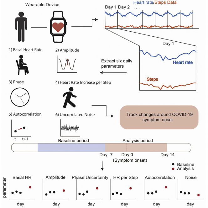
Graphical abstract

Highlights

• •We separate wearable heart rate into cardiopulmonary, circadian, and other signals
• •Parameters from different physiological systems enable disease tracking
• •Individual signals change in distinct ways around COVID-19 symptom onset
• •Together, the parameter changes can distinguish healthy from infection periods

Mayer et al. decompose wearable heart rate data to take a multidimensional view of COVID-19 disease progression. Alterations in key physiologically based parameters, such as basal heart rate, autocorrelation, circadian phase uncertainty, and the effect of activity on heart rate, occur around symptom onset.

Introduction

Wearable devices offer a unique opportunity to monitor disease and alert clinicians of deterioration that requires medical intervention in real time and at low cost.1, 2, 3, 4, 5 Moreover, wearables can be implemented in remote settings and allow for prolonged monitoring or personalized feedback to the patient and clinician about disease progression.6, 7, 8 Importantly, this feedback may help distinguish mild versus severe cases of diseases remotely when healthcare resources are limited.^4,9, 10, 11 In addition, recent work has explored how wearables may be used for real-time detection or retrospective analysis of COVID-19, for example, as a way to reduce the spread of infection.12, 13, 14, 15, 16, 17, 18, 19, 20, 21 Many of these approaches use a physiological signal from wearables, such as heart rate (HR), along with black box or machine learning methods to classify case status or disease progression.22, 23, 24

However, signals like HR reflect several physiological systems. Basal HR varies day by day within individuals and may reveal overall health. There is a strong intrinsic circadian rhythm in HR that can be characterized by a phase and amplitude. Activity increases HR in ways that vary based on pulmonary health (e.g., as measured clinically by the 6-min walk test). Hormones like cortisol increase HR on shorter timescales than circadian variation, thereby increasing the autocorrelation between HR measurements. Recently, a method has been validated to separate these physiological signals from HR.²⁵

An important remaining question is whether these separate physiological signals differentially change during illness. To test this, we collected Fitbit data before and after symptom onset of COVID-19 from 43 medical interns and 72 undergraduate and graduate students, from 2 cohorts described elsewhere.26, 27, 28 We also compared these data with a previously published dataset used for pre-detection.¹² When analyzed with our previously validated algorithm, the separate signals provided a multidimensional picture of the course of the illness, which varied between individuals who showed different symptoms. Before symptom onset, circadian rhythms were blunted, as one expects as a result of infection.²⁹ Around symptom onset, basal HR increased and its autocorrelation increased, which one would expect from a stress response due to cortisol. As the disease progressed, basal HR decreased, perhaps partially due to posture. However, HR increased more when steps were taken to meet metabolic demands. Interestingly, these increases were greatly pronounced in individuals who reported cough as a symptom, and who therefore likely had decreased pulmonary function. Taken together, these results show that one measurable signal (HR) can yield clues to how various physiological systems respond to an infection. We believe that this multifaceted approach will generate more accurate and personalized disease tracking in the future with wearables.

Results

Study overview and methodology

We adapted a validated algorithm that originally was developed to estimate daily circadian phase from wearable HR and step data.²⁵ The algorithm estimates six total parameters (see STAR Methods) each day with available data for every participant by sampling the parameter distribution using the Goodman and Weare affine invariant Markov chain Monte Carlo method.³⁰ This distribution is then used to estimate the parameter value.²⁵ Three parameters characterize the circadian phase, amplitude, and the mesor (average) of HR; one characterizes the effect of activity on HR; two characterize other factors (physiological, environmental, or external) that are known to influence HR.

For each participant, we estimated new parameter values for every day the participant had wearable HR data (see STAR Methods). In this way, for each individual, we recovered a dynamic profile of the parameters reflecting how the parameters change across the span of the study, especially before and during COVID-19 infection. For most of our analysis, we focused on a “baseline” period that was defined as −35 to −8 days before COVID symptom onset and an “analysis” period that was defined as −7 to 14 days around COVID symptom onset. Whenever possible, these periods were relative to the reported symptom date. However, if no symptom date was reported, we used the diagnosis date as a surrogate date for symptom onset. These analysis periods match similar ranges in other studies that examine wearable data around the time of symptom onset.^12,15

We analyzed participants from three independent studies^12,27,28 that collected wearable data concurrently with COVID-19 symptom and diagnosis information. A total of 29 participants were from a dataset from Mishra et al. made publicly available.¹² Data and COVID-19 symptom and diagnosis dates were obtained for 43 more participants through the Intern Health Study (IHS) out of the Michigan Neuroscience Institute.²⁷ Finally, we drew 72 participants who reported a COVID-19 diagnosis and symptoms from undergraduate and graduate students at the University of Michigan using the Roadmap mHealth platform (henceforth referred to as Roadmap-CS for college students).^26,28

In Figure S1B, we plot the number of participants separated by group that had parameter estimates for the respective day around symptom onset. A total of 89 participants (33 Roadmap-CS, 29 Mishra et al., 27 IHS) had at least 1 day with parameter estimates in the baseline and 1 day with estimates in the analysis period. In Figure S1A, we plot the data coverage for each individual separated by group around the time of symptom onset.

Daily basal HR and autocorrelated error increased at COVID symptom onset

First, we analyzed the variation in daily basal HR (parameter a; see STAR Methods: Parameter extraction from wearable heart rate and steps data) across the baseline period (days −35 to −8) and a symptomatic period (days 0–14). In Figure 1A, we plotted a sample fit from the HR algorithm (blue circles) against the data (red circles). In addition, we plotted the daily basal HR parameter when the effects of circadian timekeeping, sleep, and activity are removed (magenta line), which increased on day 0 (symptom onset) relative to the surrounding few days (Figure 1A). In general, the daily basal HR tended to increase on either the day of symptom onset or the day after in both the IHS and Mishra et al. participants (Figure 1B). Interestingly, the daily basal HR in the student group peaked 2–3 days before symptom onset (Figure 1B).

Figure 1.

Basal HR and autocorrelation increased at symptom onset in COVID patients

(A) Sample fit of the HR algorithm ±5 days around COVID symptom onset (yellow day) in one individual. The red points correspond to heart data as measured by a wearable device, while the blue points correspond to the fit from the HR algorithm. The magenta line is a plot of the daily basal HR fit from the algorithm. Note that the lower HR data typically occurred during sleep, which is removed by the HR algorithm.

(B) Daily basal HR estimates and SE of the mean from participants in each of the three study groups (blue, Roadmap-CS; red, IHS; yellow, Mishra et al. participants).

(C and D) Plot of the percentage of participants with increased basal HR (C) and autocorrelation (D) on the respective days around symptom onset compared with the basal HR and autocorrelation in the baseline period. The red bars indicate the percentage of participants with a significantly increased parameter value compared with the participant’s baseline distribution.

(E) Autocorrelation of the residuals from the HR algorithm. We computed total noise at every time point (see STAR Methods) as the difference between the daily circadian fit and the data values. Then, we fit a linear autocorrelation model to the total noise at time t + 1 versus the total noise at time t fixing the intercept at 0 (uncorrelated noise should be normally distributed around 0). The dashed dark blue lines are the mean individual linear fits during the baseline period for each individual. The dashed orange lines are the mean individual linear fits on day 1 (the day after symptom onset) for each individual. The solid lines plot the population means of the linear fits. The mean slope on day 1 (0.78) is significantly higher than the population mean slope from the baseline period (0.73, p = 0.03).

Furthermore, we computed Z scores (see STAR Methods) of the basal HR parameter for days −7 to 14 (analysis period) against the participant’s distribution from the baseline period. The individual Z scores were predominantly positive on days 0–1, where day 0 represents COVID symptom onset (Figure 1C). We quantified the increase by computing the fraction of individuals with a higher daily basal HR than their baseline average and saw a spike in this fraction on days 0–1 (Figure 1C). In addition, the fraction of participants with a significantly (i.e., p < 0.05; Figure 1C, red bars) higher daily basal HR increased on days 0–1. Moreover, the Z scores tended negative starting 3 to 4 days after symptom onset and lasting until about 13 days after symptom onset, indicating a decrease in the basal HR on those days relative to the baseline period (Figure 1C).

We saw clear trends in the autocorrelation parameter at symptom onset and after. The autocorrelated noise reflects changes in HR due to factors other than steps and the inherent circadian variation. The individual increases in the autocorrelation parameter, as represented by Z scores of the daily autocorrelation value against the participant’s baseline distribution, followed a similar trend as the dynamics of the daily basal HR. That is, at the time of symptom onset, the autocorrelation parameter increased in individual participants on days 0 and 1 (Figure 1D). However, there was no negative trend in the autocorrelation parameter in the few days after symptom onset (Figure 1D). In addition, the uncorrelated noise parameter exhibited a general decrease during the time of symptoms relative to the baseline period (Figure S3).

As the autocorrelated noise parameter reflects the amount of noise carried over to time t + 1 from time t, we fit linear models to the residuals at time t + 1 relative to t on days in the baseline period and on day 1 (Figure 1E). We fixed the intercept at zero since we assumed that the uncorrelated noise should be normally distributed with mean 0. Overall, the slopes of the fits on day 1 were significantly higher than the slopes of the fits from the baseline period (0.78 versus 0.73, p = 0.03, two-tailed t test; Figure 1E). Thus, the correlated noise increased on day 1 relative to the baseline period. Moreover, the average p value of the constant versus linear model during baseline was 0.0026 and on day 1 was 4.80 × 10⁻⁴. Therefore, the strength of the linearity of the correlated noise is also higher on day 1 relative to the baseline period.

HR per step parameter increased after symptom onset

To remove variation in HR due to activity, we fit a linear relationship between the number of steps and the HR measurement in 5-min bins (parameter d; see STAR Methods: Parameter extraction from wearable heart rate and steps data). That is, for every 5 min, we fit a linear coefficient that measures the increase in HR per step (HRpS). Before investigating the changes in the HRpS parameter around symptoms, however, we first found that the HRpS parameter negatively correlates with the daily step count (Figure S2). When we performed a linear regression of the HRpS daily parameter value versus the daily step count in each individual (see Figure S2A for a sample regression), the mean slope across individuals was −1.01 × 10⁻⁵ (p = 1.5 × 10⁻⁸; Figure S2B). Thus, in individuals, the HRpS estimate tends to increase as daily steps decrease. Moreover, we ran the same analysis using the raw data (Figures S2C and S2D) and found that the same trend occurs, indicating that this relationship between the daily effect of steps on HR negatively correlates with the daily step count in general and is not an artifact of the HR algorithm.

Since daily step counts decrease after symptom onset due to various factors, e.g., quarantining or low activity when symptomatic, we accounted for the inherent negative relationship between the HRpS parameter and the daily step count. To do this, for each individual, we computed a baseline linear relationship and used that to compute a residual for any parameter values from 0 to 14 days after symptom onset (see Figure 2A for two examples). That is, for HRpS and daily step counts from days 0 to 14, we predicted the HRpS value from the baseline linear relationship and then took the difference of the actual HRpS value and the linearly predicted value. Similar analysis was performed for the uncorrelated noise parameter and the basal HR (see STAR Methods; Figure S3). In this way, we removed the inherent decrease expected based on the lower daily step counts and isolated the effect of the symptoms on the parameter deviations.

Figure 2.

HRpS increased around COVID symptom onset

(A) Schematic of the calculation of the HRpS residual, for sample individuals. For each individual, we fit a linear relationship between the daily step counts and the HRpS parameter estimated for all days up to 10 days before symptom onset (blue dots). The red dots represent the daily step count versus HRpS pairs from days 0 to 14 after symptom onset. Then, for each daily step count and HRpS estimate pair, we compute the residual as the difference between the HRpS parameter estimate and the HRpS estimate from the predicted linear relationship. The left panel corresponds to a participant that reported cough as a symptom while the right panel participant did not.

(B) Mean HRpS residuals and SE of the mean for the respective days around COVID symptom onset in the whole population. The mean residual peaks on days 5 and 6 and is significantly greater than 0 on those days (day 5, p = 0.021; day 6, p = 0.0092).

(C) Percentage of participants with increased HRpS residual on the respective days around symptom onset compared with the baseline period. The red bars indicate the percentage of participants with a significantly increased parameter value compared with the participant’s baseline distribution.

(D) The distribution of HRpS residuals in participants that reported cough (red, mean = 0.0198) versus the distribution from those participants that did not (blue, mean = −0.0043). The mean distributions are significantly different (p = 0.018).

(E) Mean residual and SE of the mean for subjects who did report cough (red) and did not report cough (blue) on the respective days around symptom onset.

We investigated daily change in the HRpS residual after symptom onset (Figure 2B). The residual exhibited a peak on days 5 and 6 post symptom onset with both days having significantly positive mean residuals (day 5 mean = 0.036, p = 0.021; day 6 mean = 0.047, p = 0.0092). By days 13 and 14 post symptoms, the HRpS residuals decreased back to around 0. The peak in the mean HRpS residual on days 5 and 6 corresponded to the minimum mean daily step count (see Figure S2E).

HRpS residuals were significantly higher in participants exhibiting a cough

Next, we stratified participants into two groups depending on whether they reported cough as a symptom. Since symptom data were not collected as a part of the IHS, we restricted this analysis to the Roadmap-CS and Mishra et al. studies. Altogether, a total of 97 participants reported cough as a symptom while 63 did not. The mean HRpS residual from days between 0 and 14 days post symptom onset for participants reporting cough was significantly higher than residuals from participants not reporting cough (cough, mean = 0.0198; no cough, mean = -0.0043, p = 0.018; Figure 2D).

Furthermore, the daily mean HRpS residual differed between the cough and no cough groups (Figure 2E). In fact, the daily mean HRpS residual in the cough group followed a similar trend as the whole population (Figures 2B and 2C) with a peak around day 6 and a decline to around day 13 (Figure 2E). Although, the significance of the peak near day 6 was lost due to a drop in the sample size after restricting participants with cough. In contrast, the daily means of the group not reporting cough hovered around an HRpS residual of 0 for the duration of the 2 weeks post symptom onset.

Circadian phase uncertainty increased around COVID symptom onset

The HR algorithm outputs a circadian phase estimate c (i.e., the predicted time at which the basal HR is at a minimum) by taking the circular mean of all phase estimates from the sampled distribution. Then, we computed an uncertainty as the number of hours, h, such that c ± h contains 80% of the samples (Figure 3A). The uncertainty parameter acts as a surrogate measure for the strength of the circadian signal. That is, a lower uncertainty corresponds to a stronger circadian signal in the HR measurements. In Figure 3B, we plotted an actogram of HR data with the phase estimate and uncertainty from days −50 to 5 around symptom onset for one participant with an extreme change in phase. In this participant, the phase estimate became more irregular, and the uncertainty increased at the time of symptom onset. In general, we saw an increase in the mean phase uncertainty in the days leading up to symptom onset relative to the baseline period (Figure 3C).

Figure 3.

Circadian phase uncertainty increased around COVID symptom onset

(A) The HR algorithm samples the circadian phase from the posterior distribution a user-specified amount of times. The blue bars plot the histogram of circadian phase samples from 1 day of data in one example individual. The red line (5:54 a.m.) is the mean circadian phase from the sampled distribution and is taken as the estimate of the circadian phase for the day. The dashed red lines are the uncertainty bounds that correspond to the number of hours on either side of the phase estimate containing 80% of the samples (in this case, 5.61 h).

(B) Sample actogram for one participant from days −50 to 5 around COVID symptom onset. The black histogram-like bars represent HR throughout the day, i.e., thicker bars correspond to higher HR values in the 5-min bin. The actogram is double plotted; that is, the first row plots HR on day −50 and then day −49, the second row days −49 and −48, etc. The red line plots the circadian phase estimate from the HR algorithm with the shaded region representing the hours of uncertainty in that estimate. See STAR Methods and (A).

(C) The mean phase uncertainty in hours for days −35 to 14 around COVID symptom onset in the whole population. The shaded region corresponds to the SE of the mean. The uncertainty was increased when compared with our previously published algorithm because of the shorter window of data.

Machine learning successfully classified healthy versus pre-symptomatic periods

To investigate the extent to which the parameters varied between particular pre-symptomatic periods, we ran the parameters from two classes in a linear support vector machine (SVM) classification learner. In particular, we used the 6 parameter estimates from 55 participants having data on every day from days −10 to −6 (class 1, early pre-symptomatic) and days −5 to −1 (class 2, infection periods) (Figure 4A): basal HR, autocorrelated noise, HRpS residual, circadian phase uncertainty, amplitude, and uncorrelated noise. Then, we trained a linear SVM model on the dataset using 5-fold cross-validation. Note that the method in this figure is not currently intended as real-time detection. Instead, we wished to further evaluate the parameter changes that occur around COVID-19 symptom onset, and examine whether machine learning could detect these changes.

Figure 4.

A linear support vector machine model successfully classifies early pre-symptomatic periods versus infection periods

(A) Schematic for our machine learning analysis. Two classes were passed into a linear support vector machine classification learner: class 1 consisting of individual parameter estimates on days −10 to −6 (P_-10, …, P_-6) and class 2 consisting of individual parameter estimates on pre-symptomatic days −5 to −1 (P_-5, …, P_-1). A total of 55 of the 89 individuals met our requirements for the pre-symptomatic machine learning classification.

(B–E) Receiver operating characteristic (ROC) curve when using only the amplitude (B), circadian phase uncertainty (C), basal HR (D), or autocorrelated noise (E) parameter as a feature.

(F) ROC curve when using all parameters (basal HR, HRpS residual, autocorrelated and uncorrelated noise, amplitude, and circadian phase uncertainty) as features.

Overall, the parameter estimates exhibited significant power in differentiating these two classes. Specifically, when we used only amplitude, the model was able to distinguish between classes 1 and 2 with an area under the curve (AUC) of 0.71 (Figure 4B), which was higher than the AUC for uncertainty (0.67; Figure 4C), basal HR (0.65; Figure 4D), and autocorrelation (0.58; Figure 4E). Altogether, when we used all parameters, the estimated AUC was 0.75 with the linear SVM classifier. When compared with several simple baseline features of HR, the combination of all parameters from the HR algorithm had higher overall performance in terms of the AUC (Figure S4C). Moreover, we ran the same procedure to instead distinguish between a longer healthy baseline period (days −21 to −14) and a symptomatic period (days 0 to 7). We recovered an AUC of 0.86 when using all six parameters (Figure S4E). Interestingly, a majority of the result with all parameters was due to the basal HR (Figure S4F). Other commonly used classifiers were also tested with the healthy baseline and symptomatic periods (Figures S4J and S4K): random forest had an AUC of 0.75, and logistic regression had an AUC of 0.68.

Discussion

In a sizable cohort of COVID-positive individuals with wearable data from three separate studies, we showed that key parameters modeling the variation in HR, whether related to circadian, activity, or other factors, changed around symptom onset. In particular, we saw increases in the basal HR at symptom onset and the day after. As fever is a common symptom of COVID patients,^5,31 we hypothesize that a portion of the increase in basal HR is a result of the increase in HR that occurs while individuals are in a febrile state.³² Moreover, individuals may have heightened stress and anxiety around symptom onset, especially given the increased fear of contracting COVID due to the pandemic. Any increase in stress or anxiety may manifest as a sustained increase in average HR. Interestingly, the increase in basal HR occurred earlier in the Roadmap-CS population, peaking several days before symptom onset. This could be due to physiological differences between the groups, or the fact that the symptom date for the student cohort was obtained retrospectively at the end of the study, often long after the symptoms occurred and longer than retrospective collection in the IHS study. The retrospective nature of these data could have increased bias in the reported symptom onset date, leading to the observed shift. In addition, basal HR generally dropped off a few days after symptom onset, potentially due to changes in posture (e.g., more time spent lying down).

Furthermore, we saw increases in the autocorrelation parameter at symptom onset and the day after. The autocorrelation parameter is a marker for the changes in HR due to mechanisms other than circadian variation, such as hormone release, postural changes (e.g., prolonged standing), eating, light input, and caffeine intake. Like the initial increase in basal HR, we expect that the spike in the autocorrelation around symptom onset is due to sustained elevated stress related to cortisol. Hence, tracking autocorrelation could be valuable to better understand disease progression, although the parameter may not be best suited for future real-time prediction (see Figure 4). We also note that the autocorrelation increase could have cumulative effects, as the parameter represents a quantity of noise carried over from one point to the next.

As activity contributes significantly to acute variation in HR, we removed the effect of steps on HR by fitting a linear coefficient that models the increase in HR due to one step. Relatedly, previous research has explored the relationship between steps and heart rate through neural networks to predict variables related to health.³³ When examining our HRpS parameter, however, we found that it negatively correlated with the daily step count. Since an individual naturally tends to take fewer steps after symptom onset (due to quarantine procedures, increased fatigue, etc.), we accounted for this relationship by examining the residuals. After doing this, we still see significant elevations in the HRpS residual on days 5 and 6 after symptom onset. Similar significant effects, even after accounting for total steps, were seen for the basal HR and the uncorrelated noise parameter. The increase in the HRpS may reflect a heightened cardiac load while recovering from symptoms, meaning that a larger increase in heart rate occurs in response to activity during the disease or recovery than when compared with a healthy baseline. In particular this increase may be related to decreased respiratory function, since participants who listed cough as a symptom had an HRpS residual consistently higher than those who did not.

In addition, we saw increases in the uncertainty of the circadian phase in the days leading up to and around COVID symptom onset. Since the phase uncertainty parameter relates to the strength and consistency of the circadian component of the HR rhythm, these pre-symptomatic changes may correspond to early signs of infection that disrupt the underlying circadian signal. Alternately, increased circadian disruption could lead to a greater likelihood of COVID infection and development of symptoms. However, the timing of this deviation in the uncertainty speaks to the potential of our multifaceted algorithm to capture pre-symptomatic changes through parameter analysis. Unlike the HRpS residual that changes days after symptom onset, the circadian uncertainty could be a strong candidate for future pre-detection.

Previous studies reveal the potential of using wearables to predict symptoms before they occur or to differentiate between COVID-positive and -negative cases, both important in fighting the current pandemic and, more generally, ushering in a new era of personalized medicine.³⁴ However, by accounting for circadian variation, removing data during sleep, and extracting the effect of activity on HR, our work allows for a more detailed tracking of the physiological effects of an infection. Taking this multipronged perspective enables us to extract more meaningful information that can be used to understand the impact of the disease on different physiological systems. Indeed, we show that the one signal of HR can be decomposed into multiple parameters of potential interest for tracking disease. Our platform provides an important step as a way to potentially distinguish circadian variation and effects due to activity from other physiological changes that result from COVID or similar diseases.

Limitations of the study

This study works with a large cohort of COVID-19-positive study participants and does not consider other influenza-like illnesses. Indeed, previous work has shown that similar changes in wearable HR data occur in both COVID and flu patients.³⁵ Therefore, future work is needed to determine if the parameter deviations we observed serve as unique signatures of COVID or persist in other illnesses. In terms of the deviation in the autocorrelation parameter around symptom onset, a key future direction would be to refine the current model to separate out the physiological or environmental factors that differentially change during infection. In addition, since we compiled data from three separate studies, we were not able to investigate the effect of covariates, such as age, gender, or BMI. Future work is needed to explore the impact of these factors on the observed parameter changes.

Another limitation is that, due to not having full date information for some of the data, we were not able to directly account for seasonality effects in the data. This could be an important consideration for future disease prediction work based on these results. Missing data is another challenge when working with wearable devices, and ensuring sufficient data quality was an issue, particularly in the machine learning analysis. Furthermore, the machine learning task undersampled healthy periods, by focusing on parameter classification between specific windows and thereby balancing the class sizes. A potential real-time detection system would typically use an imbalanced dataset, with many more healthy periods than sick periods (making the prediction task more challenging). While this does not undermine the claim that machine learning can successfully distinguish between these periods, future work is needed to assess performance over longer time spans. Finally, this work does not aim to build up a real-time detection system for COVID or general infections; indeed, we detect some of the parameter changes (e.g., for the HRpS residual) at or after symptom onset and the data normalization for each participant is done retrospectively. Instead, carefully examining and tracking parameter changes around symptom onset is a necessary first step to using this framework to build such a system in the future.

STAR★Methods

Key resources table

.

REAGENT or RESOURCE	SOURCE	IDENTIFIER
Deposited data
Processed daily metrics	This paper	https://github.com/mayercl/heart_rate_covid
Software and algorithms
MATLAB	The Mathworks Inc.	https://www.mathworks.com/
HR algorithm code for disease tracking	This paper	https://github.com/mayercl/heart_rate_covid

Resource availability

Lead contact

Further information and resource requests should be directed to and will be fulfilled as possible by the lead contact, Daniel B. Forger (forger@umich.edu).

Materials availability

This study did not generate new physical materials or reagents.

Experimental model and subject details

Intern health study data

Participants were drawn from the 2019 and 2020 cohorts of the Intern Health Study.²⁷ The Intern Health Study (IHS) is a multi-site cohort study that follows physicians across several institutions in their first year of residency. The intern participants entered residency in 2018 and were contacted via e-mail 2–3 months before residency onset regarding details of the study and provided informed written consent to participate. All subjects were invited to wear a Fitbit Charge 2 to track sleep patterns, heart rate, and physical activity. From April to December of 2020, interns were asked to report any potential COVID-19 symptoms and whether they were tested along with the results. For analysis, we included individuals who reported a COVID positive test, symptoms, and had wearable data anywhere from 50 days before symptom onset to 14 days after.

Mishra et al. dataset

Data was downloaded through the data availability link provided in.¹²

Roadmap college student (Roadmap-CS) dataset

This study examined student health and well-being during the altered 2020–2021 academic year in addition to biospecimen collection, wearable data from a Fitbit Charge 3, and self-reported COVID-19 diagnosis and symptom information gathered retroactively. A total of 2,164 undergraduate and graduate students were enrolled between September 2020 and January 2021.^26,28 The study was approved by an Institutional Review Board at the University of Michigan Medical School (HUM00185391). Students were given a Fitbit Charge 3 upon enrollment in the study and instructed to wear the watch for at least 8 hours per day up to at least 5 days per week. The study team had access to the participant’s Fitbit data through the Roadmap 2.0 app. The app was developed by S.W.C. to interface with the Fitbit app and to promote health (physical and mental) and well-being through a menu of resilience-building activities, based upon principles of positive psychology. In an exit survey participants were asked to report (among other information) COVID-19 testing dates, symptom onset dates, and symptom information. For analysis, we included individuals who reported a COVID positive test, symptom information, symptom date or test date, and all wearable data collected during the time of the study.

Method details

Data processing

For all participants, we removed any heart rate data that were measured during sleep events reported by the wearable device. As some wearable devices do not track sleep events, e.g., Apple Watch, we also added a constant steps filter that removed any heart rate data when zero total steps were recorded in an interval of more than two hours. Then, we binned the heart rate data into 5-minute intervals by averaging over all heart rate data in the bin. For each 5-min bin of the heart rate data, we also computed an average step count in that bin by averaging over all steps data. Finally, we parsed the heart rate data into days and fit the parameters (see below) on each day.

Parameter extraction from wearable heart rate and steps data

Model equation and parameters

For each participant and day, we fit the following model to the heart rate and steps data binned into 5-min intervals:

$$\text{HR}=a-b\cdot \cos \left(\frac{\pi }{12}\left(\text{Time}-c\right)\right)+d\cdot \text{Activity}+\epsilon ,$$

where a is the basal HR in beats per minute (bpm), b is the amplitude of the circadian oscillation in HR (which may be 0 if such an oscillation does not exist), c is the time in hours of the circadian minimum of the heart rate rhythm (i.e., circadian phase), d is the increase in HR per unit activity (steps), and ε is the model error.

We account for two sources of noise known to contribute to the error ε. First, heart rate measurements often have inherent device noise, i.e., they can differ from ECG data by up to 30 beats per minute.³⁶ Additionally, other factors affect heart rate on the hour timescale, e.g., cortisol and other hormones, which are influenced by a range of stimuli. These effects are distinct from the cardiac demand from activity modeled by the parameter d. We account for these other factors in two additional parameters: a parameter σ, which is a measurement of independent noise, and a parameter k, which is a correlated component, measuring errors on longer timescales. Ultimately, we assume ε follows an AR(1) process:

$${\epsilon }_{t+1}=k{\epsilon }_t+\text{N}\left(0,{\sigma }^2\right),$$

i.e., the noise at time t+1 carries over a fraction k of the noise at time t plus independent Gaussian noise with standard deviation σ (representing measurement error and new external effects). All six parameters, including the two noise parameters, are fit directly from the data.

Parameter estimation with Bayesian uncertainty quantification

To estimate the six parameters, we use the Goodman and Weare ensemble Markov Chain Monte Carlo (GWMCMC)³⁰ sampler with affine invariance which provides error estimates and handles large gaps in the data. Large gaps are common in wearable data (e.g., because of charging), and some methods such as least-squares are biased by these gaps.³⁷ On the first day of data, the six parameters are sampled from the likelihood using GWMCMC. On successive days, the posterior is sampled instead of the likelihood from a prior distribution which is the previous day’s fit with Gaussian noise with standard deviation of 1 h.²⁵

Modification of algorithm for disease detection

Our published method analyzes daily wearable heart rate data to determine daily parameters indicating the state of several physiological systems. We found that several refinements of the algorithm increased its accuracy in disease detection:

• (1)The original algorithm used the waking data on either side of a sleep episode resulting in up to 48 hours' worth of data, and discarded all data during sleep. We now consider the non-sleep data just within one 24-h period. Since typically 16 h or less of data are used, the uncertainty of the phase parameter increases compared with the original method. However, this allows for detection on shorter time intervals.
• (2)Total daily steps can decrease after infection (See Figure S2). There is an inherent bias in binned wearable data where parameters like HRpS depend on the total number of steps taken over a day. This bias occurs even if one directly fits the parameter to the raw data reported by the device rather than with our algorithm (See Figure S2). This bias occurs because if activity stops at the end of a bin, the next bin will still see an increased heart rate. All wearable data are binned, so the effect of activity on heart rate lingers after the activity is finished. This increases the basal heart rate, decreases the HRpS, and also increases the uncorrelated noise parameter. While we tried several methods to correct each bin, the most effective way was to fit a linear relationship between the total number of steps during a day and these parameters and account for it in our analysis. See Figure 2.
• (3)Postural effects could also be important. When activity is low, this causes a lower heart rate than predicted by our linear model. We fitted an indicator to bins with low activity (<= 1 step per minute) to account for this. While this did lower the AIC in many individuals, it did not affect parameters like circadian uncertainty but did affect the parameters discussed above. The effect can also be efficiently accounted for daily, assuming walking typically occurs at the same cadence, with the method described above and in Figure 2.

Accounting for these effects did not change the time course of parameters changes with COVID infection (See Figures S2 and S3). However, because of the more considerable impact of total steps on HRpS, we used its modified value (residual) in our analysis in Figures 4 and S4.

Quantification and statistical analysis

Computing Z-scores and statistical analysis

We used as a baseline distribution the parameter estimates from days -35 to -8. Then, Z-scores for the parameter estimates on days -7 to 14 were calculated by normalizing by the baseline distribution. For example, the Z-score for the circadian amplitude parameter on day 0 was calculated in the following way:

$${\underset{¯}{z}}_{d,0}=\left(d_0-{\mu }_d\right)/{\sigma }_d,$$

where d₀ is the circadian amplitude estimate on day 0, μ_d the mean circadian amplitude in the baseline distribution, and σ_d the standard deviation of the circadian amplitude baseline distribution.

We determined the fraction of individuals with an increase in a parameter relative to the baseline by taking the number of individuals with a positive Z-score over the total number of individuals that had data to estimate the parameter on that day. Of the individuals with a significant increase in the parameter, we further investigated whether the increase was significant by performing a two-tailed t-test comparing the parameter estimate on that specific day to the individual’s baseline distribution of that parameter.

Total noise linear regression

For all subjects, we computed residuals as the difference between the HR data and the value predicted by the model in the Model equation and parameters subsection above). Then, for each individual and each day, we fit a linear relationship between the residual at t and the residual at t+1 (to simulate the autocorrelated error). We used the function fitlm in Matlab R2020b to fit the linear model and required at least 10 data points in the day for a fit. We specified a zero intercept because we assume that the uncorrelated noise should be normally distributed around zero. Then, we computed the mean slope for each individual in the baseline period (Figure 1E, blue lines). In total, 68 participants had at least one slope during the baseline period. A total of 59 participants had enough data to estimate a slope on day 1 post symptoms (Figure 1E, orange lines). Finally, we compared the mean slopes during the baseline period with those on day 1 with a two-tailed t-test (ttest2 function in Matlab R2020b).

HRpS residual

For each individual, we predicted the linear relationship between the daily step count and the daily HRpS parameter estimate. In particular, for all days before 10 days before symptom onset, we used fitlm in Matlab R2020b to fit a linear relationship to the daily step count versus the daily HRpS parameter (see Figure S2A for an example). The distribution of slopes obtained is significantly less than zero (ttest2 in Matlab R2020b). Then, we computed the HRpS residuals for each daily step count and daily HRpS parameter as the difference between the estimated HRpS parameter and the value obtained from the estimated linear relationship. We used the function feval in Matlab R2020b to evaluate the individual’s linear fit at the specific daily step count.

Raw data steps to heart rate analysis

For each individual and each day, we estimated the slope, m, and intercept of a linear relationship between the 5-minute bin step mean and the 5-min bin heart rate mean (using fitlm in Matlab R2020b, Figure S2C, top). Next, we aggregated all pairs of daily step count and slope m and fit a new linear relationship with these pairs, again using fitlm (Figure S2C, bottom). We assessed whether the distribution was significantly less than zero using a two-tailed t-test (ttest2 in Matlab R2020b).

Machine learning classification

We separated the dataset into two groups, depending on the analysis. For example, (i) a healthy group taken from days -21 to -14 around symptom onset and (ii) a symptomatic group taken from days 0 to 7 (Figures S4D–S4K). A total of 48 of the 89 participants that had parameter estimates on every day in both periods were included for the analysis. Next, we scaled the parameters by normalizing by the individual mean after merging both the healthy and symptomatic groups. For example, we scaled the basal heart rate for participant i on day j by dividing by a where a is the mean basal heart rate after combining the participant’s basal heart rates in the healthy and symptomatic periods.

Next, we constructed vectors of predictor and response variables using the scaled parameter estimates. In particular, the feature vectors for class 1 were of the form

(a_-21, …, a_-14, b_-21, …, b_-14, k_-21, …, k_-14, σ_-21, …, σ_-14, d_-21, …, d_-14, u_-21, …, u_-14),

where a represents the basal heart rate, b the amplitude, k the autocorrelated noise, σ the uncorrelated noise, d the HRpS, and u the circadian phase uncertainty. Similarly, the feature vectors for class 2 were of the form

(a₀, …, a₇, b₀, …, b₇, k₀, …, k₇, σ₀, …, σ₇, d₀, …, d₇, u₀, …, u₇).

Similar feature vectors were used in the pre-symptomatic classification procedure (Figure 4). Then, we used the Classification Learner App provided in the Statistics and Machine Learning Toolbox in Matlab R2020b to train a linear support-vector machine model to all the data with 5-fold cross validation, a box constraint level equal to 1, and an auto kernel scale mode. In Figure S4J, we trained a random forest model using 5-fold cross validation, a maximum number of splits equal to 95, and 30 learners. We also used 5-fold cross validation for logistic regression (Figure S4K).

We compared the results from the scaled parameter with those generated from other summary statistics of heart rate data, using the linear support-vector machine model (Figures S4A–S4C). The mean, standard deviation, and maximum features are determined by computing these measurements on the raw heart rate data on a daily basis, while the resting heart rate (RHR) proxy is computed by taking the daily mean of 5-minute binned HR measurements for which no steps occurred in the previous 15 min. To test whether the AUCs were significantly different, we performed a bootstrapping approach, wherein for each iteration we sample with replacement from the feature vectors to construct sets of new feature vectors of equal size. We repeat this process for n = 1000 iterations, in order to generate a distribution of AUCs.

Additional resources

Intern Health Study portal: https://www.srijan-sen-lab.com/intern-health-study.

Published: April 19, 2022

Data and code availability

• •The dataset from Mishra et al. is publicly available via the data availability link provided in the reference. All processed daily metrics used in this study can be found at the publicly available repository (https://github.com/mayercl/heart_rate_covid).
• •All code used in this study can be found at the publicly available repository (https://github.com/mayercl/heart_rate_covid).
• •Any additional information needed to reanalyze the data reported in this paper will be made available when possible by the lead contact upon request.

References

- 1.Li X., Dunn J., Salins D., Zhou G., Zhou W., Schüssler-Fiorenza Rose S.M., et al. Digital health: tracking physiomes and activity using wearable biosensors reveals useful health-related information. PLoS Biol. 2017;15:e2001402. doi: 10.1371/journal.pbio.2001402. [DOI] [PMC free article] [PubMed] [Google Scholar]
- 2.Cox S.M., Lane A., Volchenboum S.L. Use of wearable, mobile, and sensor technology in cancer clinical trials. JCO Clin. Cancer Inform. 2018;2:1–11. doi: 10.1200/CCI.17.00147. [DOI] [PubMed] [Google Scholar]
- 3.Dunn J., Runge R., Snyder M. Wearables and the medical revolution. Per Med. 2018;15:429–448. doi: 10.2217/pme-2018-0044. [DOI] [PubMed] [Google Scholar]
- 4.Ming D.K., Sangkaew S., Chanh H.Q., Nhat P.T.H., Yacoub S., Georgiou P., et al. Continuous physiological monitoring using wearable technology to inform individual management of infectious diseases, public health and outbreak responses. Int. J. Infect. Dis. 2020;96:648–654. doi: 10.1016/j.ijid.2020.05.086. [DOI] [PMC free article] [PubMed] [Google Scholar]
- 5.Smarr B.L., Aschbacher K., Fisher S.M., Chowdhary A., Dilchert S., Puldon K., et al. Feasibility of continuous fever monitoring using wearable devices. Sci. Rep. 2020;10:21640. doi: 10.1038/s41598-020-78355-6. [DOI] [PMC free article] [PubMed] [Google Scholar]
- 6.Badgeley M.A., Shameer K., Glicksberg B.S., Tomlinson M.S., Levin M.A., McCormick P.J., et al. EHDViz: clinical dashboard development using open-source technologies. BMJ Open. 2016;6:e010579. doi: 10.1136/bmjopen-2015-010579. [DOI] [PMC free article] [PubMed] [Google Scholar]
- 7.Daniels J., Georgiou P. IEEE Biomedical Circuits and Systems Conference (BioCAS); 2019. A Data-Driven Detection System for Predicting Stress Levels from Autonomic Signals; pp. 1–4. [Google Scholar]
- 8.Radin J.M., Quer G., Ramos E., Baca-Motes K., Gadaleta M., Topol E.J., et al. Assessment of prolonged physiological and behavioral changes associated with COVID-19 infection. JAMA Netw. Open. 2021;4:e2115959. doi: 10.1001/jamanetworkopen.2021.15959. [DOI] [PMC free article] [PubMed] [Google Scholar]
- 9.Khichar S., Midha N., Bohra G.K., Kumar D., Gopalakrishanan M., Kumar B., et al. Healthcare resource management and pandemic preparedness for COVID-19: a single centre experience from Jodhpur, India. Int. J. Health Pol. Manag. 2020;9:493–495. doi: 10.34172/ijhpm.2020.102. [DOI] [PMC free article] [PubMed] [Google Scholar]
- 10.Seshadri D.R., Davies E.V., Harlow E.R., Hsu J.J., Knighton S.C., Walker T.A., et al. Wearable sensors for COVID-19: a call to action to harness our digital infrastructure for remote patient monitoring and virtual assessments. Front. Digital Health. 2020;2:8. doi: 10.3389/fdgth.2020.00008. [DOI] [PMC free article] [PubMed] [Google Scholar]
- 11.Natarajan A., Su H.-W., Heneghan C. Assessment of physiological signs associated with COVID-19 measured using wearable devices. NPJ Digit Med. 2020;3:156. doi: 10.1038/s41746-020-00363-7. [DOI] [PMC free article] [PubMed] [Google Scholar]
- 12.Mishra T., Wang M., Metwally A.A., Bogu G.K., Brooks A.W., Bahmani A., et al. Pre-symptomatic detection of COVID-19 from smartwatch data. Nat. Biomed. Eng. 2020;4:1208–1220. doi: 10.1038/s41551-020-00640-6. [DOI] [PMC free article] [PubMed] [Google Scholar]
- 13.Alavi A., Bogu G.K., Wang M., Rangan E.S., Brooks A.W., Wang Q., et al. Real-time alerting system for COVID-19 using wearable data. medRxiv. 2021 doi: 10.1101/2021.06.13.21258795. Preprint at. [DOI] [PMC free article] [PubMed] [Google Scholar]
- 14.Yamagami K., Nomura A., Kometani M., Shimojima M., Sakata K., Usui S., et al. Early detection of symptom exacerbation in patients with SARS-CoV-2 infection using the Fitbit Charge 3 (DEXTERITY): pilot evaluation. JMIR Form Res. 2021;5:e30819. doi: 10.2196/30819. [DOI] [PMC free article] [PubMed] [Google Scholar]
- 15.Quer G., Radin J.M., Gadaleta M., Baca-Motes K., Ariniello L., Ramos E., et al. Wearable sensor data and self-reported symptoms for COVID-19 detection. Nat. Med. 2021;27:73–77. doi: 10.1038/s41591-020-1123-x. [DOI] [PubMed] [Google Scholar]
- 16.Miller D.J., Capodilupo J.V., Lastella M., Sargent C., Roach G.D., Lee V.H., et al. Analyzing changes in respiratory rate to predict the risk of COVID-19 infection. PLoS One. 2020;15:e0243693. doi: 10.1371/journal.pone.0243693. [DOI] [PMC free article] [PubMed] [Google Scholar]
- 17.Hirten R.P., Danieletto M., Tomalin L., Choi K.H., Zweig M., Golden E., et al. Longitudinal physiological data from a wearable device identifies SARS-CoV-2 infection and symptoms and predicts COVID-19 diagnosis. medRxiv. 2020 doi: 10.2196/26107. http://medrxiv.org/lookup/doi/10.1101/2020.11.06.20226803 Preprint at. [DOI] [PMC free article] [PubMed] [Google Scholar]
- 18.D’Haese P.-F., Finomore V., Lesnik D., Kornhauser L., Schaefer T., Konrad P.E., et al. Prediction of viral symptoms using wearable technology and artificial intelligence: a pilot study in healthcare workers. PLoS One. 2021;16:e0257997. doi: 10.1371/journal.pone.0257997. [DOI] [PMC free article] [PubMed] [Google Scholar]
- 19.Liu S., Han J., Puyal E.L., Kontaxis S., Sun S., Locatelli P., et al. Fitbeat: COVID-19 estimation based on wristband heart rate using a contrastive convolutional auto-encoder. Pattern Recognit. 2022;123:108403. doi: 10.1016/j.patcog.2021.108403. [DOI] [PMC free article] [PubMed] [Google Scholar]
- 20.Richards D.M., Tweardy M.J., Steinhubl S.R., Chestek D.W., Hoek T.L.V., Larimer K.A., et al. Wearable sensor derived decompensation index for continuous remote monitoring of COVID-19 diagnosed patients. NPJ Digit Med. 2021;4:155. doi: 10.1038/s41746-021-00527-z. [DOI] [PMC free article] [PubMed] [Google Scholar]
- 21.Changes in vital data after a COVID-19 infection. Corona Data Donation - Scientific Analysis. 2021. https://corona-datenspende.de/science/en/reports/prolongedchanges/
- 22.Nestor B., Hunter J., Kainkaryam R., Drysdale E., Inglis J.B., Shapiro A., et al. Dear watch, should I get a COVID-19 test? Designing deployable machine learning for wearables. medRxiv. 2021 doi: 10.1101/2021.05.11.21257052. Preprint at. [DOI] [Google Scholar]
- 23.Merrill M.A., Althoff T. Transformer-based behavioral representation learning enables transfer learning for mobile sensing in small datasets. arXiv. 2021 http://arxiv.org/abs/2107.06097 Preprint at. [Google Scholar]
- 24.Grzesiak E., Bent B., McClain M.T., Woods C.W., Tsalik E.L., Nicholson B.P., et al. Assessment of the feasibility of using noninvasive wearable biometric monitoring sensors to detect influenza and the common cold before symptom onset. JAMA Netw. Open. 2021;4:e2128534. doi: 10.1001/jamanetworkopen.2021.28534. [DOI] [PMC free article] [PubMed] [Google Scholar]
- 25.Bowman C., Huang Y., Walch O.J., Fang Y., Frank E., Tyler J., et al. A method for characterizing daily physiology from widely used wearables. Cell Rep. Methods. 2021;1:100058. doi: 10.1016/j.crmeth.2021.100058. [DOI] [PMC free article] [PubMed] [Google Scholar]
- 26.Gilley K.N., Baroudi L., Yu M., Gainsburg I., Reddy N., Bradley C., et al. Risk factors for COVID-19 in college students identified by physical, mental, and social health reported during the fall 2020 semester: observational study using the Roadmap app and Fitbit wearable sensors. JMIR Ment. Health. 2022;9:e34645. doi: 10.2196/34645. [DOI] [PMC free article] [PubMed] [Google Scholar]
- 27.Sen S., Kranzler H.R., Krystal J.H., Speller H., Chan G., Gelernter J., et al. A prospective cohort study investigating factors associated with depression during medical internship. Arch. Gen. Psychiatry. 2010;67:557–565. doi: 10.1001/archgenpsychiatry.2010.41. [DOI] [PMC free article] [PubMed] [Google Scholar]
- 28.Cislo C., Clingan C., Gilley K., Rozwadowski M., Gainsburg I., Bradley C., et al. Monitoring beliefs and physiological measures in students at risk for COVID-19 using wearable sensors and smartphone technology: protocol for a mobile health study. JMIR Res. Protoc. 2021;10:1–9. doi: 10.2196/29561. [DOI] [PMC free article] [PubMed] [Google Scholar]
- 29.Mazzoccoli G., Vinciguerra M., Carbone A., Relógio A. The circadian clock, the immune system, and viral infections: the intricate relationship between biological time and host-virus interaction. Pathogens. 2020;9:83. doi: 10.3390/pathogens9020083. [DOI] [PMC free article] [PubMed] [Google Scholar]
- 30.Goodman J., Weare J. Ensemble samplers with affine invariance. Commun. Appl. Maths. Comput. Sci. 2010;5:65–80. [Google Scholar]
- 31.Zhou F., Yu T., Du R., Fan G., Liu Y., Liu Z., et al. Clinical course and risk factors for mortality of adult inpatients with COVID-19 in Wuhan, China: a retrospective cohort study. Lancet. 2020;395:1054–1062. doi: 10.1016/S0140-6736(20)30566-3. [DOI] [PMC free article] [PubMed] [Google Scholar]
- 32.Karjalainen J., Viitasalo M. Fever and cardiac rhythm. Arch. Intern. Med. 1986;146:1169–1171. [PubMed] [Google Scholar]
- 33.Spathis D., Perez-Pozuelo I., Brage S., Wareham N.J., Mascolo C. Proceedings of the Conference on Health, Inference, and Learning. New York, NY, USA. Association for Computing Machinery; 2021. Self-supervised transfer learning of physiological representations from free-living wearable data; pp. 69–78. [Google Scholar]
- 34.Tyler J., Choi S.W., Tewari M. Real-time, personalized medicine through wearable sensors and dynamic predictive modeling: a new paradigm for clinical medicine. Curr. Opin. Syst. Biol. 2020;20:17–25. doi: 10.1016/j.coisb.2020.07.001. [DOI] [PMC free article] [PubMed] [Google Scholar]
- 35.Shapiro A., Marinsek N., Clay I., Bradshaw B., Ramirez E., Min J., et al. Characterizing COVID-19 and influenza illnesses in the real world via person-generated health data. Patterns (N Y). 2021;2:100188. doi: 10.1016/j.patter.2020.100188. [DOI] [PMC free article] [PubMed] [Google Scholar]
- 36.Wang R., Blackburn G., Desai M., Phelan D., Gillinov L., Houghtaling P., et al. Accuracy of wrist-worn heart rate monitors. JAMA Cardiol. 2017;2:104–106. doi: 10.1001/jamacardio.2016.3340. [DOI] [PubMed] [Google Scholar]
- 37.Huang Y., Bowman C., Walch O., Forger D. 2019 13th International Conference on Sampling Theory and Applications. SampTA; 2019. Phase estimation from noisy data with gaps; pp. 1–4. [Google Scholar]
Associated Data
This section collects any data citations, data availability statements, or supplementary materials included in this article.
Supplementary Materials
Data Availability Statement