Plasticity of Multidimensional Receptive Fields in Core Rat Auditory Cortex Directed by Sound Statistics

Abstract

Sensory cortical neurons can nonlinearly integrate a wide range of inputs. The outcome of this nonlinear process can be approximated by more than one receptive field component or filter to characterize the ensuing stimulus preference. The functional properties of multidimensional filters are, however, not well understood. Here we estimated two spectrotemporal receptive fields (STRFs) per neuron using maximally informative dimension analysis. We compared their temporal and spectral modulation properties and determined the stimulus information captured by the two STRFs in core rat auditory cortical fields, primary auditory cortex (A1) and ventral auditory field (VAF). The first STRF is a dominant, sound feature detector in both fields. The second STRF preferred lower modulations and had less spike information compared to the first STRF. The information jointly captured by the two STRFs was larger than that captured by the individual STRF, reflecting nonlinear interactions of two filters. This information gain was larger in A1. We next determined how the acoustic environment affects the structure and relationship of these two STRFs. Rats were exposed to moderate levels of spectrotemporally modulated noise during development. Noise exposure strongly altered the spectrotemporal preference of the first STRF in both cortical fields. The interaction between the two STRFs was reduced by noise exposure in A1 but not in VAF. The results reveal new functional distinctions between A1 and VAF indicating that (i) A1 has stronger interactions of the two STRFs than VAF, (ii) in both fields, noise exposure diminishes modulation parameter representation contained in the noise more strongly for the first STRF, and (iii) plasticity induced by noise exposure can affect the strength of filter interactions in A1. Taken together, ascertaining two STRFs per neuron enhances the understanding of cortical information processing and plasticity effects in core auditory cortex.

INTRODUCTION

The auditory receptive field (RF) is commonly estimated as a single filter capturing spectrotemporal features of sounds that preferentially activate a neuron. By estimating a spectrotemporal receptive field (STRF), basic neural sound processing aspects have been revealed (e.g., Blake and Merzenich 2002; Elhilali et al. 2004; Gourévitch et al. 2009). Spike-triggered averaging (STA) of stimulus envelopes that precede a spike has been one of the widely utilized estimators of sound feature preferences (de Boer and Kuyper, 1968; Theunissen et al., 2000; Depireux et al., 2001; Woolley et al., 2005). Nonlinear processing by neurons, however, is not well captured by a single STRF alone (Sahani and Linden, 2003; Machens et al., 2004) and has been generally approximated as a static linear filter followed by a nonlinear input-output function (de Ruyter van Steveninck and Bialek, 1988; Marmarelis, 1997; Ringach, 2004; Simoncelli et al., 2004; Meyer et al., 2016). Recent studies demonstrated that auditory cortical neurons can be more fully characterized by RFs and nonlinearities with higher dimensionality thus revealing that many central auditory neurons can encode more than one stimulus feature and that those multiple features can interact in a nonlinear fashion to increase stimulus representation (Atencio et al., 2008; Harper et al., 2016; Kozlov and Gentner, 2016; Atencio and Sharpee, 2017; Rahman et al., 2019). Therefore, it can be more insightful for the study of the auditory forebrain (Shih et al., 2020) to use neuronal models that utilize multiple, independent descriptive filters and their joint input-output function (“nonlinearity”). In addition, interactions between the multiple filters can nonlinearly increase the encoded stimulus information over that of the independent filters (Atencio et al., 2008; Shih et al., 2020). While some fundamental differences between the concurrent filters have been revealed, such as systematically different latencies and properties of the associated nonlinearities (Atencio et al., 2008, 2009; Sharpee et al., 2011; Shih et al., 2020), potential biologically meaningful differences in the encoded stimulus features have remained elusive.

In this study, we aimed to expand our understanding of multidimensional RFs properties by characterizing the functional features of each RF dimension and the interactions between the different dimensions. To that end, we utilized maximally informative dimension (MID) analysis (Sharpee et al., 2004; Atencio et al., 2008) to capture the first two RF dimensions, the input-output functions, and their interactions (“two-filter model”). MIDs are obtained based on maximizing mutual information, a quantitative metric to estimate the dependence of a response on the evoking stimulus, and can incorporate nonlinear aspects of neuronal processing without being affected by stimulus correlations. Previously, we showed that the MID two-filter model was more informative than the STA or the single-filter model and the stimulus information represented by the two-filter model was more pronounced in cortex than in thalamus or midbrain (Atencio et al., 2008, 2009, 2012; Shih et al., 2020). The high resemblance of the first MID to the STA indicated that the first filter can be interpreted as a sound feature detector that dominates the function of a neuron. While some systematic relationships between the two filters have been suggested (Atencio et al., 2008, 2009; Sharpee et al., 2011), basic stimulus features encoded by the second dimension that modestly add to the total information captured in the two-filter model have not been described in detail. We hypothesized that the two filters encode distinct functional stimulus domains.

Our first objective was to compare MID features between different auditory cortical regions that have shown some functional distinctions in their STA. We examined multidimensional RFs in the core fields, primary auditory cortex (A1) and ventral auditory field (VAF), of rats. A1 and VAF both receive major lemniscal thalamocortical projections from the ventral division of medial geniculate body but from largely nonoverlapping distribution of thalamic neurons (Polley et al., 2007; Storace et al., 2010, 2011). Their anatomical and functional distinctions are similar to those seen between the sharply and broadly tuned regions of cat A1 (Read et al., 2001, 2011). As mammalian cortical subfields have distinct roles in sound processing, rat A1 and VAF reveal different specializations in temporal processing, sound discrimination, and stimulus specific adaptation (Engineer et al., 2015; Nieto-Diego and Malmierca, 2016; Osman et al., 2018). We hypothesized that functional differences between these regions in their first filter are also reflected by systematic differences in the second filter.

The second objective was to assess whether sound-exposure induced similar cortical plasticity affects in both MIDs and whether the filter interactions can be altered. We estimated MIDs from animals that were raised in moderately noisy environments. Changes of RF properties, such as frequency tuning or temporal preference, have been observed for animals reared in a modified sound environment (e.g., Chang and Merzenich, 2003; Insanally et al., 2009; Oliver et al., 2011; Pysanenko et al., 2018). Our recent study showed that plastic changes of STA properties depend on the exposure-noise statistics (Homma et al., 2020). Here we hypothesized that the second filter also changes following noise exposure but that the interaction between the two MIDs remains unaffected.

We found that (i) the interaction of the first and second filters was stronger in A1 than in VAF, (ii) the first, dominant filters in A1 preferred slightly lower temporal and spectral modulation frequencies than in VAF, and (iii) the second filters consistently preferred lower temporal and spectral modulation frequencies than the first filters in both fields. Furthermore, we showed that (iv) the interaction of the first and second filters decreased with noise exposure in A1, and (v) noise exposure altered the temporal and spectral modulation preferences for the first MIDs and, similarly but to a lesser degree, for the second MIDs. The results support the idea that A1 and VAF are distinct and parallel sound processing pathways and that experience-induced plasticity can affect the feature preference of both MIDs as well as their degree of interaction.

EXPERIMENTAL PROCEDURES

All experimental procedures involving animals were approved by the Institutional Animal Care and Use Committee (IACUC) at the University of California San Francisco and were carried out in accordance with NIH guidelines.

Noise synthesis

All sound stimulus generation and data analysis were performed using MATLAB (Mathworks). We synthesized an unbiased dynamic moving ripple (DMR) that contained 50 sinusoidal carrier frequencies per octave (0.5 to 40 kHz) with random phases. Spectrotemporal envelopes were generated with a maximum of 4 cyc/oct spectral modulation frequencies (SMFs), a maximum of 40 Hz temporal modulation frequencies (TMFs), and a maximum 40 dB spectrotemporal modulation depth (Escabi and Schreiner, 2002; Atencio et al., 2008). We prepared two biased DMRs (Homma et al., 2020). One was restricted to modulations of 5 to 20 Hz ‘high’ TMFs and 0 to 0.3 cyc/oct ‘low’ SMFs, and the other was limited to 0 to 5 Hz ‘low’ TMFs and 0.3 to 2 cyc/oct ‘high’ SMFs. We refer to the biased DMRs as “high-TMF-low-SMF-noise” and “low-TMF-high-SMF-noise”, respectively.

Experimental model and noise rearing

This study used thirty-eight female Sprague-Dawley rats (Charles River, wild type). Seventeen of them (17/38) were raised in a sound-shielded test chamber while presenting a biased noise (either high-TMF-low-SMF- or low-TMF-high-SMF- noise) from postnatal day 6 (P6). The noise was presented to rat litters 24 h/d at a sound level of ~60 dB SPL from a loudspeaker. Modulation biases were selected based on rat vocalization modulation power spectra (Homma et al., 2020) to examine the developmental plasticity of different noise statistics. The litters were housed with their mother, and none showed signs of abnormal behavior. The remaining twenty-one animals (21/38) were raised in a typical rat colony environment. After weaning, for all of the groups, animals were co-housed in groups of 2–3 to enhance social interaction under a 12 h light/12 h dark cycle. At the end of noise-rearing, extracellular unit recordings were performed (age: P79–152, weight: 242–330g). For the Control group with no noise exposure, recordings were performed at matching ages to the experimental groups. A subset of animals (19/38) was trained in a behavioral task but their physiological data were pooled with untrained animals of the same exposure condition since the effect of training was much smaller than the effect of noise-exposure (Homma et al., 2020). The duration of noise exposure was ~2 months for untrained animals or ~3–4 months for trained animals. Some data were presented previously for charactering exposure effects on A1 STAs (Homma et al., 2020). In the present study, we focus on the MID analysis in A1 and VAF.

Electrophysiological recording

The procedures were described in detail previously (Homma et al., 2020). Briefly, anesthesia was induced with ketamine hydrochloride (100 mg/kg) and xylazine hydrochloride (3.33 mg/kg), and maintained with a mixture of ketamine (10–50 mg/kg) and xylazine (0–20 mg/kg). Atropine sulphate, dexamethasone sodium phosphate and meloxicam were administered for therapeutic purposes. Lidocaine hydrochloride was used prior to incisions. Following a tracheotomy, the skin and muscle over one hemisphere of the auditory cortex was removed, a craniotomy window (3 mm × 5 mm) was made, and the dura was removed. Silicone oil was used to cover the cortex.

Auditory stimulus presentation and neural data acquisition were computer controlled using RHD2000 Interface software (Intan Technologies). All sound stimuli were presented once contralaterally using an electrostatic speaker (EC1, Tucker-Davis Technologies) at a 96 kHz sampling rate. Target locations were selected based on pure tone mapping (tungsten electrodes) of the tonotopic gradient of A1 and VAF (Polley et al., 2007). We pseudorandomly presented 675 different pure tones (50 ms, 0.5–32 kHz in 0.13 octave steps, 0–70 dB SPL in 5 dB increments). We typically identified the frequency border of A1 and VAF after 20–30 sites. Once high frequency areas (20–30 kHz) of the two fields were identified, we inserted a multi-contact silicon probe array (Neuronexus or Cambridge NeuroTech) perpendicularly to the pial surface to a depth of ~ 0.9 to 1.35 mm and presented an unbiased DMR at 70 dB SPL for 20 min. The probe had 32 or 64 recording sites vertically arranged with 20 or 50 μm dorso-ventral spacing and 50 μm medio-lateral intervals.

Neural traces were band-pass filtered between 0.5 and 6 kHz and digitized at 20 kHz sampling rate. Single units were identified offline using MountainSort (Chung et al., 2017).

Estimation of spectrotemporal receptive field

For analysis, we downsampled the ripple stimulus (unbiased DMR) to a resolution of 0.1 octave and 5 ms. We used reverse correlation (spike-triggered averaging, STA) to obtain STRFs by averaging 100 ms of spectrotemporal stimulus envelope immediately preceding a spike (Escabi and Schreiner, 2002; Atencio and Schreiner, 2010, 2016). Next, we used MID analysis to obtain multidimensional RFs (Sharpee et al., 2004, 2006; Atencio et al., 2008). We divided the data into four segments for a jackknife estimate. For each estimate, a different 3/4 of the data was used as training data set. The remaining 1/4 of the data was used as test data set. The first MID (MID1) was estimated with iterations to maximize mutual information between stimulus and spike train. The second MID (MID2) was estimated by searching the stimulus space for another receptive component that increased the information over MID1 alone. The iterations for MID2 were terminated when the information on the test set using the estimated MID2 achieved a maximum and before the information decreased while the information from the training set continued to increase. This early-stopping procedure limits over-fitting.

To calculate the mutual information between stimulus and spikes, each stimulus segment S that evoked a spike was projected onto a filter V using the inner product z = s·V with V representing STA, MID1 or MID2. The projection values (z) were then binned to compute the probability distribution P_V (z|spike). Positive projection values indicate that high-energy portions of the stimulus fall on excitatory parts of the filter and low-energy portions on inhibitory parts of the filter. Negative values mean that stimulus and filter are anti-correlated. The prior stimulus distribution, P_V (z), was estimated by projecting all stimuli onto the filter V regardless of a spike occurrence. To normalize the projection values, the units of P_V (z|spike) and P_V (z) were transformed to standard deviation using x = (z – μ)/σ, where μ and σ are the mean and standard deviation of P_V (z).

The nonlinearity is a characterization of the input-output function for each filter and was estimated as $P_V(\mathit{\text{spike}}|x) = P_V\left(\mathit{\text{spike}}\right)\frac{P_V(x|\mathit{\text{spike}})}{P_V\left(x\right)}$, where P_V (spike) is the average firing rate of the neuron (Agüera y Arcas et al., 2003).

The mutual information for a filter V and single spikes was estimated using the following function:

$$I\left(V\right) = \int dx{P}_V(x|\mathit{\text{spike}})lo{g}_2\left[\frac{P_V(x|\mathit{\text{spike}})}{P_V\left(x\right)}\right].$$ (1)

The joint mutual information for the two MIDs was determined as

$$I\left(MID1,MID2\right) = \iint dx1,dx2P_{MID1,MID2}(x1,x2|\mathit{\text{spike}})lo{g}_2\left[\frac{P_{MID1,MID2}(x1,x2|\mathit{\text{spike}})}{P_{MID1,MID2}\left(x1,x2\right)}\right].$$ (2)

x1 and x2 represent the projection values of the stimulus onto the first and second dimensions, MID1 and MID2, respectively. P_{MID1, MID2} (x1, x2) presents the prior probability distribution of dimension MID1 and MID2, and P_{MID1, MID2} (x1, x2 | spike) is the probability distribution calculated only from the stimulus segments that evoked a spike.

The information value for unlimited data size was estimated by extrapolating the information values to infinite data set size. We calculated information values over 90–100% of test data set (1/4 of the data set) in 2.5% increments for each segment. The information calculated for the fractioned data was plotted against the inverse of the data fraction percentage (1/90, 1/92.5, 1/95, 1/97.5, 1/100), a linear fit was made, and the y-intercept was the estimated information value for the test set.

“MID1 contribution” was defined as $100\times \frac{I\left(MID1\right)}{I\left(MID1,MID2\right)}$, and the “synergy” between the two MIDs was defined as $100\times \frac{I\left(MID1,MID2\right)}{I\left(MID1\right)+I\left(MID2\right)}$, where each mutual information value was obtained via the extrapolation procedure.

Analysis of receptive field properties

Single units were included for the following analyses only when they had information values larger than the 95th percentile of the null distribution for the first MID, I(MID1), and for the joint filter, I(MID1,MID2). We estimated a population null distribution by reversing in time the stimulus envelope and computing MIDs relative to this statistically identical signal that is uncoupled in time from the response. In addition, we excluded the units with <100 spikes for a segment in the jackknife procedure to avoid convergence failures during the MID information extrapolation estimate. The median firing rate of the units analyzed was 2.67 spike/s (25–75th percentile range: 1.50 to 5.31 spike/s; corresponding to 1800–6372 spikes in total). Consistency of the RF structure was evaluated using a reliability index, which is the average correlation coefficient for the four segments of the jackknife procedure. Significance (P < 0.05) was established regarding a null distribution of correlations obtained from STRFs of time-reversed spike trains. We also computed the reliability index values for STAs with this method and confirmed that it was comparable to the index values that have previously been used for STA (r = 0.92, p < 0.001) but is not feasible for MIDs, in which a null distribution was obtained for each unit by shuffling spike-times relative to the stimulus envelope and recalculating the STA (Escabí et al., 2014).

Characteristic frequency (CF), response latency, bandwidth (BW), and sharpness of tuning (Q) values were obtained from each STA, MID1 and MID2 (Atencio and Schreiner, 2012). The reliability of these measures is proportional to the reliability index obtained for the RFs as a whole. Typically, only the excitatory portion of STRFs is used to determine CF, latency, BW and Q. In contrast to STA and MID1, however, MID2 consistently has a symmetric nonlinearity, i.e., a neuron is responding when the stimulus is either positively or negatively correlated with the MID2, reflecting a 180° envelope phase response invariance (Atencio et al., 2008). We, therefore, used both excitatory and inhibitory portions after converting the magnitude of each STRF bin to absolute values for constructing the marginal distribution for estimating basic STRF characterization in all STAs, MID1s and MID2s. CF was identified as a peak value of each filter after summing it along the time axis for STA or MID1. BW was computed as the width of the summed function where it exceeded 30% of its maximum value. Response latency was obtained as the peak time of each filter after summing it along the frequency axis. Q value for STRFs was obtained by dividing CF by BW, both of which were estimated from the responses to continuous broadband DMR at ~70 dB SPL. Based on local energy estimates, the STRF Q value corresponded approximately to Q30 of tonal tuning curves. We confirmed that the CF, latency and Q values estimated after converting to absolute values were comparable to the values conventionally estimated from the excitatory portion for STA and MID1 (r_s = 0.4 to 0.7, P < 0.001). Only a small statistically significant difference between the two methods was found for latency and Q for both STA and MID1 (paired non-parametric t-test, P < 0.005) but not for CF (P > 0.3). This reflects slightly longer response latency and narrower tuning for the inhibitory portion than the excitatory portion (Atencio and Schreiner, 2012). The median difference was 1 ms for latency and 0.2–0.3 for Q.

Ripple transfer functions (RTFs) were computed using the 2D Fourier transform of each STA, MID1 or MID2 (Escabi and Schreiner, 2002; Atencio and Schreiner, 2010, 2016). Each ripple transfer function was summed along the spectral modulation axis or along the temporal modulation axis, and the peak values were reported as best temporal and spectral modulation frequency, respectively.

Population ripple transfer function (pRTF) was estimated as an average of the normalized individual RTFs (Homma et al., 2020). To determine significant differences between pRTFs, we divided each pRTF into six equal areas for comparing the two cortical fields. For comparing control and noise-reared animals, each pRTF was separated into nine areas based on three DMR noise parameter ranges (spectral modulation frequency ranges: 0 to 0.3, 0.3 to 2, 2 to 4 cyc/oct, temporal modulation frequency ranges: 0 to 5, 5 to 20, 20 to 40 Hz). Each pRTF comprises 16 by 16 bins with the resolution of 0.26 cyc/oct and 2.67 Hz. Absolute values of differences between pRTFs were calculated for each bin, and mean values were computed as an average of the values for the bins that represent the six or nine divided areas, respectively. Similarly, the simulated differences were generated by shuffling group labels of individual RTFs, for the corresponding six or nine areas. We compared the actual and simulated differences and obtained P values as a proportion of the fraction of simulated differences that exceeded the actual difference, for the total number of simulated values (n=10000) with Bonferroni correction. In order to control for unbalanced sampling numbers, we resampled the data with replacement using the smallest number of units for the compared groups as sampling size.

Statistical analysis

Non-parametric methods were used for all statistical analysis. For comparing two cortical fields, Rank-sum (also known as Mann-Whitney-U) and Kolmogorov-Smirnov (KS) tests were used. Bonferroni adjustment was used for all multiple comparisons. For comparing properties of three filters (STA, MID1 and MID2), Friedman test, a non-parametric one-way ANOVA with repeated measures, was used followed by Dunn’s test for post hoc comparisons. For comparing control and two noise-exposed groups, Kruskal-Wallis (KW) test, a non-parametric one-way ANOVA on ranks, was used, followed by Dunn’s test for post hoc comparisons. For correlation analysis, Spearman’s rho (r_s) value was computed.

RESULTS

I. Spectro-temporal filter properties in A1 and VAF

We identified two core auditory cortical fields, A1 and VAF (Figure 1A), in ketamine-xylazine-anesthetized rats based on the reversal of the CF gradient and response properties to tonal stimuli (Polley et al., 2007). Then, we presented broadband DMR noise to the contralateral ear. For estimating STRFs, we utilized two methods (Figure 1B). First, a spike-triggered average (STA) was computed, i.e., the average of the spectrotemporal stimulus envelopes that preceded a spike (Aertsen and Johannesma, 1981; DeCharms et al., 1998; Theunissen et al., 2000; Escabi and Schreiner, 2002; Atencio and Schreiner, 2010) (two examples are presented in Figure 1B, 1st column). Second, using the MID approach (Sharpee et al., 2004; Atencio et al., 2008), we obtained multidimensional RFs based on mutual information estimation (see Methods). The first filter, MID1, captures the majority of information between spikes and stimulus (Figure 1B, 2nd column). Adding estimation of a second filter (Figure 1B, 3rd column), MID2 further maximizes the joint mutual information that is simultaneously computed based on the two filters while the first filter remains essentially unchanged (Atencio et al., 2008). For each filter, we computed a nonlinearity (Figure 1C), expressing the spiking probability as a function of the similarity between the stimulus and the filter, which characterizes the rule of transforming inputs to outputs (Sharpee, 2013). The similarity between the stimulus and the filter was estimated by computing the correlation (“projection value”) between the stimulus’ spectrogram immediately preceding a spike and the spectrotemporal receptive field (STA, MID1, or MID2) and normalized to z-scores (see Methods). STA and MID1 show an asymmetric nonlinearity, i.e., only positive correlations between stimulus and filter can yield an increase in firing rate. By contrast, the MID2 nonlinearity is generally symmetric, which means spikes were evoked when stimulus envelope and filter were either correlated or anti-correlated. Although MID2 is a generally weaker and less structured filter, it is capturing an effective stimulus dimension that is not represented by STA or MID1. Furthermore, we computed the joint, two-dimensional nonlinearity for MID1 and MID2, which is the probability of spike occurrence as a function of the projection values simultaneously projecting the stimulus onto the two filters, and estimated its ability of capturing nonlinear interactions of the two filters (Figure 1D). Generally, the two-dimensional nonlinearity showed a non-separable, usually crescent-shaped function due to the asymmetric shape of the MID1 nonlinearity and the symmetric shape for the MID2 nonlinearity. The joint nonlinearity reflects how the filters cooperate and generate synergistic effects at specific stimulus configurations (Atencio et al., 2008).

Figure 1.

Examples of spectrotemporal receptive fields and associated nonlinearities.

(A) Schematic of rat brain. The positions of five auditory fields are indicated on the auditory cortex. The magnified window shows the frequency gradient reversal at the border of A1 and VAF. A, anterior; A1, primary auditory cortex; AAF, anterior auditory field; D, dorsal; H, higher frequency region; L, lower frequency region; P, posterior; PAF, posterior auditory field; SRAF, suprarhinal auditory field; V, ventral; VAF, ventral auditory field. Scale bars: 1 mm. (B-D) Spectrotemporal receptive fields (STRFs) or filters obtained using spike-triggered average (STA) (B, 1st column) or maximally informative dimension (MID) analysis (B, 2nd and 3rd columns) for a single neuron. Each row represents a neuron. The information value estimated for each filter is shown at the top of each plot with an indication of significance (*) or non-significance (n.s.). Nonlinearities or input-output functions of STA (C, pink in left column) or the first dimension of MID analysis, MID1 (C, cyan in left column), are asymmetric, i.e., firing rates are elevated only for positive correlations (projection values) between stimulus and filter. Nonlinearities of the second dimension of MID analysis, MID2 (C, right column), are symmetric indicating 180° envelope phase invariance of spike generation. Two-dimensional nonlinearities of the joint derivation of the two MIDs are shown in D. (E) Information values were similar for STA and MID1. (F) Information captured by MID2 was smaller than for MID1. (G) Information captured by the two-filter (MID12) model exceeds that for the single filter (MID1) model.

Figure 2.

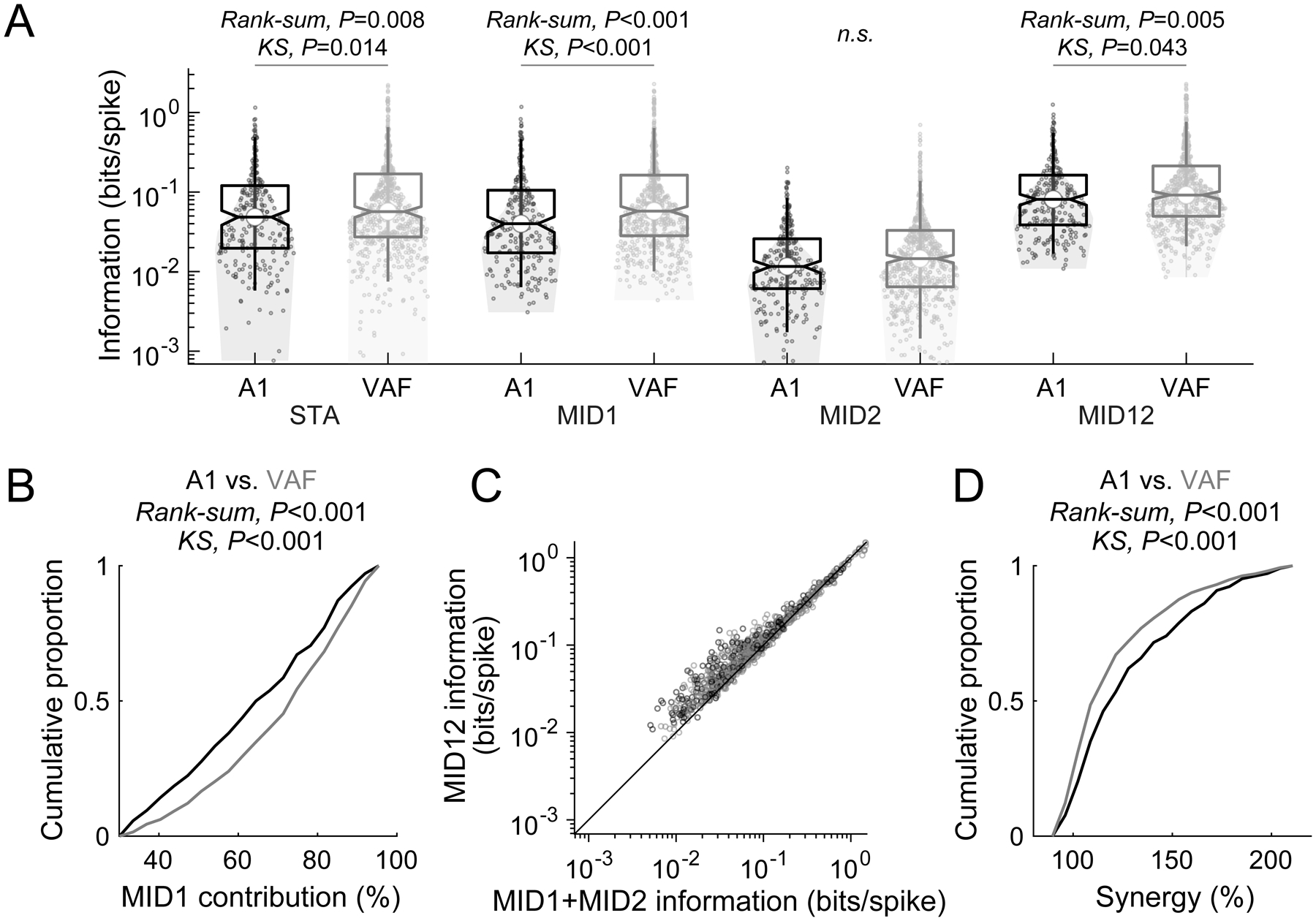
Comparison of stimulus information captured by single-filter and two-filter models in A1 and VAF.

(A) VAF showed larger information values than A1 for STA, MID1 and MID12. Box plots of median values plus 25th-75th percentiles of information values with the 5th-95th percentiles depicted by whiskers. Horizontal lines above the box plots indicate statistically significant differences. (B) MID1 contribution $\left(100\times \frac{MID1 \mathit{\text{information}}}{MID12 \mathit{\text{information}}}\right)$ was larger for VAF than A1. (C) The information captured by the two-filter model (MID12) was larger than the sum of the two filters (MID1+MID2). (D) Synergy $\left(100\times \frac{MID12 \mathit{\text{information}}}{MID1+MID2 \mathit{\text{information}}}\right)$, indicative a cooperative gain of the joint two-filter model (MID12) over the sum of the two individual filters (MID1+MID2), was larger in A1 than VAF.

Figure 3.

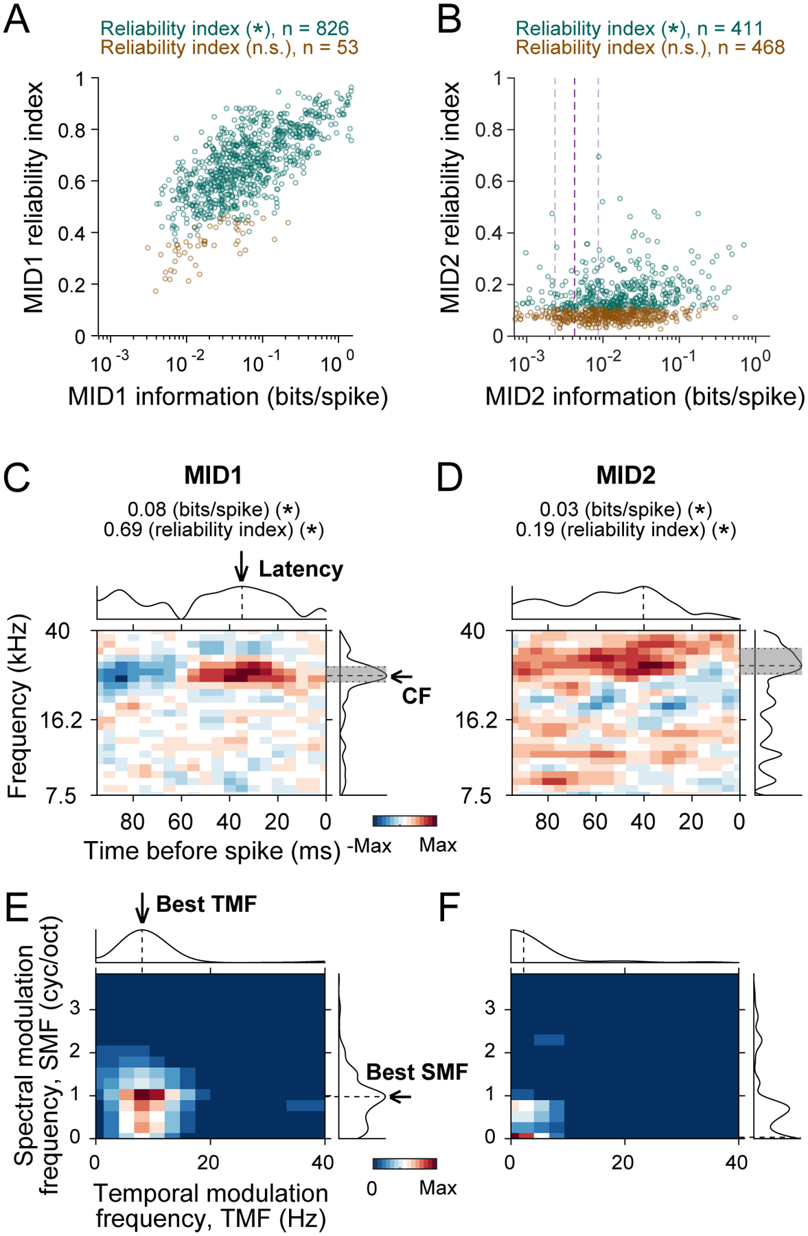
Filter reliability and parameter derivation.

(A-B) Reliability index, a measure of the reproducibility of filter estimation, was computed for MID1 (A) and MID2 (B) and plotted against the corresponding information value of each neuron. The number of units with significant (*) or non-significant (n.s.) reliability index is shown in the heading. The dashed lines in B indicate 25th, 50th and 75th percentiles of MID2 information values. (C-D) Examples of MID1 (C) and MID2 (D) and their marginal distributions of response magnitude (absolute values). Characteristic frequency (CF) and latency are indicated by black arrows and dashed lines in the marginal distributions with bandwidth (BW) shown by gray shading and dotted lines. Information value and reliability index are indicated at the top. All of them were significant (*). (E-F) Ripple transfer functions and the marginal distributions of modulation power for the MID1 (C) and MID2 (D) is shown in E and F, respectively. Best spectral and temporal modulation frequencies (best SMF and TMF) are indicated by black arrows and dashed lines in the marginal distributions.

The amount of stimulus information captured by a single filter (STA, MID1 or MID2) or the joint filter (MID12) was estimated by calculating their mutual information (see Methods). The analysis was restricted to units that had significant MID1 and MID12 to ensure successful fitting to the model (A1, n = 243; VAF, n = 636). Significance was assigned when the information value of real data exceeded the 95th percentile of the null distribution (see Methods). As the filter structures of STA and MID1 were similar, their information values were highly correlated (r_s = 0.95, P < 0.001) (Figure 1E). The outliers were mostly units with non-significant STA (red in Figure 1E; A1, n = 12; VAF, n = 29). By design of the MID method, MID1 has larger information values than MID2, and their information values were more loosely correlated (r_s = 0.70, P < 0.001) (Figure 1F) compared to STA and MID1 (Figure 1E). Only 70% of units with significant MID1 had a significant MID2 (green in Figure 1F; A1, n = 165; VAF, n = 444). Low information for MID2, however, does not imply the absence of a second filter since the filter is designed to increase the joint information via a non-separable two-dimensional nonlinearity. Accordingly, the information values for joint processing, MID12, were larger than those of MID1 even when neurons had non-significant MID2 information values (Figure 1G) (r_s = 0.95, P < 0.001). The information gain for the joint filters was relatively larger for units with lower single-filter information.

MID1 and MID2 show stronger cooperation in A1 than in VAF

We next compared information values of STA, MID1, MID2 and MID12 between the two auditory cortical fields based on 879 single units (A1, n = 243; VAF, n = 636; Figure 2A). Information values of STA, MID1 and MID12 were significantly higher for VAF compared to A1 with a similar trend for MID2 (STA: +17% increase of median for VAF vs. A1, Rank-sum, P = 0.008, KS, P = 0.014; MID1: +44%, Rank-sum, P < 0.001, KS, P < 0.001; MID2: +25%, Rank-sum, P = 0.054, KS, P = 0.11; MID12: +13%, Rank-sum, P = 0.005, KS, P = 0.043).

To illustrate the role of interaction between the two filters, as captured by the two-dimensional nonlinearity, we computed two values. The “MID1 contribution” is the proportion of MID1 information relative to MID12 information (Figure 2B). The MID1 contribution was +13% higher for VAF (median: A1, 60%; VAF, 73%) (Rank-sum, P < 0.001, KS, P < 0.001). This indicates that MID1 accounts for a greater proportion of the two-filter information in VAF compared to A1. A similar conclusion can be drawn from computing the “synergy,” defined as the joint MID12 information value divided by the sum of the individual information values of MID1 and MID2, an indicator of the cooperativity of the two filters. The joint MID12 information values were generally larger than the sum of the information values of MID1 and MID2 (Figure 2C). The proportion of neurons that exceeded 100% of synergy was 85% (n=206) for A1 and 73% (n=462) for VAF. Comparison between A1 and VAF showed that synergy was larger for A1 (median, 123%) than for VAF (109%) (Rank-sum, P < 0.001, KS, P < 0.001) (Figure 2D). This higher degree of synergy in A1 may be a consequence of its lower MID1 information values compared to VAF since synergy was generally larger for the units with relatively low information values (Figure 2C). In summary, these findings show that a cooperative multi-filter model captures more stimulus-based information than single-filter models. By considering a second, independent stimulus dimension, we found that the synergistic cooperativity between the two filters differed between two, generally quite similar core cortical fields, A1 and VAF.

We next assessed properties of MID1 and MID2 based on their STRF structure to illuminate some specific, stimulus-related properties of the filters for the two cortical fields. To verify stability of STRF structure, we first computed a reliability index (average of STRF correlations between jackknife subsets; see Methods). Reliability indices for MID1 showed strong correlation to the MID1 information (r_s = 0.70, P < 0.001; Figure 3A). 94% of the units had a significant MID1 filter structure (n = 826). The reliability index for MID2 was lower but still significant for ~50% of the neurons (n=411; Figure 3B). The reliability index correlation with the MID2 information was also weaker (r_s = 0.22, P < 0.001). We extracted stimulus-related response properties only for structurally significant filters (MID1: A1, n = 223 VAF, n = 603; MID2: A1, n = 98; VAF, n = 313). To understand basic response properties of STRFs, CF, latency, and Q values were extracted from the marginal distributions (Figure 3C–D). The robustness of these estimates is proportional to the reliability index. Furthermore, we estimated modulation preferences from ripple transfer functions (RTFs) (Figure 3E–F) and evaluated their differences between the two fields. RTFs were obtained by 2D Fourier transform of STRFs (Escabi and Schreiner, 2002; Atencio and Schreiner, 2010, 2016), and best temporal and spectral modulation frequencies were extracted (see Methods).

As the difference of unit numbers with structurally significant filters between MID1 and MID2 indicate, about half of the units with significant MID1 reliability indices was not accompanied by MID2s with significant reliability indices (A1, n = 132; VAF, n = 296). There were, however, no consistent statistical differences between units with or without structurally significant MID2 for CF, latency, Q, and best temporal and spectral modulation frequency values. The exceptions were only found in temporal aspects of VAF neurons with minor differences. Compared to the neurons with a structurally non-significant MID2, the neurons with a structurally significant MID2 showed slightly smaller MID1 latency by 2.7 ms and slightly higher MID1 best temporal modulation frequency by 0.3 Hz (Rank-sum, P < 0.01). Thus, we compare the response property values of STRF and RTF for MID1 without considering the significance of MID2 structure in the following analyses.

A1 has shorter latency and broader tuning than VAF

For MID1 and MID2, the targeted frequency range of the two fields was well-matched (Rank-sum, KS, P > 0.05 for all) (Figure 4A–B), as assessed by the CFs of MID1 and MID2. The observation that MID2 CFs were shifted by 1/2–1 octave relative to MID1 CFs matches previous observations in the cat (Shih et al., 2020). The preponderance of MID2 CF shifts toward lower value is likely related to the fairly high CF target range in this study. MID1 latencies (cyan lines and plots in Figure 4C–D) in A1 were slightly shorter than in VAF (Rank-sum, P = 0.03; KS, P = 0.004). MID2 latencies were significantly longer than for MID1 for both fields, with the largest difference for A1 (Atencio et al., 2008; Shih et al., 2020). MID1 Q values, indicative of tuning sharpness, were higher for VAF than A1 (Rank-sum, KS, P < 0.001 for both) (cyan lines and plots in Figure 4E–F). These observations are consistent with previously reported RF differences between these fields (Polley et al., 2007; Lee et al., 2016; Osman et al., 2018) and support the argument that response properties extracted from MID1 accurately reflect physiological differences between the two fields as estimated by other methods, confirming their distinct processing properties. By contrast, MID2, the second filter, showed no significant difference between A1 and VAF for CF, latency, or Q (Rank-sum, KS, P > 0.05 for all) (olive lines and plots in Figure 4), suggesting that their contribution may be related to more global roles of stimulus processing that are less field-specific.

Figure 4.

Basic response characteristics of MID1 and MID2 in A1 and VAF.

(A, C, E) Cumulative proportion of CF (A), latency (C) and Q (=CF/BW) (E) are plotted for each filter and field (MID1 for A1, cyan; MID1 for VAF, light cyan; MID2 for A1, olive; MID2 for VAF, light olive). (B, D, F) Box plots showing median values plus 25th-75th percentiles of CF (B), latency (D) and Q (F). Horizontal lines mark statistically significant differences. *, P < 0.05; ***, P < 0.001. (A and B) There was no statistical difference of sampled CFs between A1 and VAF. CFs of MID2 were lower than that for MID1 for both fields. (C and D) Latencies for MID1 were slightly longer for VAF than for A1. MID2 showed distinctly longer latencies than MID1 in both fields. (E and F) Q values were larger for VAF than A1, indicating that VAF had narrower frequency tuning. MID2 tuning was markedly broader compared to MID1.

VAF prefers higher temporal and spectral modulations than A1

To understand potential differences of stimulus-envelope modulation preferences in the two cortical fields, best temporal and spectral modulation frequencies were extracted from the ripple transfer functions and compared between A1 and VAF for STA, MID1 and MID2, respectively (Figure 5A–B).

Figure 5.

Spectral and temporal modulation properties of the three filters for A1 and VAF.

(A and B) Box plots of median values plus 25th-75th percentiles of best temporal modulation frequencies (TMFs) (A) or best spectral modulation frequencies (SMFs) (B) for A1 (black; STA, n = 226, MID1, n = 223, MID2, n = 98) and VAF (grey; STA, n = 605, MID1, n = 603, MID2, n = 313). Horizontal lines above the box plots indicate statistically significant differences. n.s., Not significant. (A) VAF preferred slightly higher TMFs than A1. (B) STA and MID1 had higher SMFs in VAF than in A1. (C-E) Population ripple transfer functions (pRTFs, 1st and 3rd columns) and distribution of best modulation frequencies (2nd and 4th columns) for STA (C), MID1 (D) and MID2 (E) for A1 (1st and 2nd columns) and VAF (3rd and 4th columns) neurons, respectively. The contour plots in the 2nd and 4th columns represent the modulation power in the pRTFs. The difference of pRTFs between VAF and A1 is shown in the 5th column. Color bar indicates normalized modulation power strength or differences.

To examine the differences between the three filters, we analyzed only the units with significant reliability index for all the STA, MID1 and MID2 (A1, n = 89, VAF, n = 300). Generally, STA and MID1 showed similar modulation preference although MID1 preferred slightly lower temporal and higher spectral modulations compared to STA (best TMFs: Friedman, X² > 89.80, P < 0.001; post hoc, P < 0.01; best SMFs: Friedman, X² > 19.49, P < 0.001; post hoc, A1, P > 0.05, VAF, P < 0.001). Both best temporal and spectral modulation frequencies were significantly lower for MID2 compared to STA or MID1 (post hoc, P < 0.001 for all).

To compare the two fields, we included all the structurally significant filters (STA: A1, n = 226 VAF, n = 605; MID1: A1, n = 223 VAF, n = 603; MID2: A1, n = 98; VAF, n = 313) (Figure 5A–B). For STA or MID1, VAF consistently showed higher values than A1 for both best temporal and spectral modulation frequencies (Rank-sum, KS, P < 0.001 for all). For MID2, best temporal modulation frequency was only slightly higher for VAF (Rank-sum, P = 0.002, KS, P = 0.004), however, no statistical difference was found between A1 and VAF for best spectral modulation frequency (Rank-sum, P = 0.096, KS, P = 0.36).

Population profiles of the modulation preference (Figure 5C–D) also show that VAF has moderately higher temporal and spectral modulation frequency values than A1 for STA and MID1, reflected in the difference plots between the two fields (Figure 5C–D, 5th column). Although weak, a similar trend of slightly higher temporal and spectral modulation frequencies for VAF was observed for MID2 (Figure 5E). Overall, modulation-preference differences between the two fields were consistent for STA, MID1 and MID2.

Taken together, the main functional differences between A1 and VAF are manifested in STA or MID1 but not strongly in MID2. In both fields, STA and MID1 prefer substantially higher temporal and spectral modulation values than MID2. These fundamental differences in stimulus preference between MID1 and MID2 were expressed in both fields, supporting that the two filters preferentially encode different stimulus domains. MID1 is selective for a specific range of moderately high spectral and temporal modulations, commonly found in vocalizations of rats and other species (Theunissen et al., 2000), with a high degree of feature selectivity, as manifested by asymmetric nonlinearities. By contrast, MID2 modulation preferences are below the main vocalization range and not dependent on envelope-phase as reflected in the symmetric nonlinearity. This suggests that MID2 adds responsiveness to coarsely distributed spectral content with slow temporal modulations that may signal dynamic context and background conditions.

II. Effects of background noise exposure

Functional plasticity is an important attribute of cortical processing and has been widely demonstrated for tone- and noise-derived receptive fields (for review: Fritz et al. 2007; Froemke and Schreiner 2015; Osmanski and Wang 2015). It has not been shown, however, whether plasticity similarly affects higher-dimensional receptive fields and whether the nonlinear interactions seen in two-filter models are also affected. We therefore assessed the influence of plasticity induced by different environmental background noises on the structures and information contents of the two MID filters. For the plasticity experiments, we generated two biased DMR noises (Figure 6A–C) that differed in their distribution of temporal and spectral modulation frequencies from the spectrotemporal modulations commonly found in rat vocalizations (Homma et al., 2020). One noise contained ‘high’ temporal modulation frequencies (TMFs) from 5 to 20 Hz and ‘low’ spectral modulation frequencies (SMFs) from 0 to 0.3 cyc/oct (shown in orange in Figure 6A), and the other noise was composed of ‘low’ temporal modulation frequencies from 0 to 5 Hz and ‘high’ spectral modulation frequencies from 0.3 to 2 cyc/oct (shown in green in Figure 6A). Then, we raised rat pups in one of the biased DMR noises at a moderate sound level (~60 dB SPL) starting at P6 to cover their auditory critical period (de Villers-Sidani and Merzenich, 2011). Noise exposure was extended throughout their early adulthood to maximize the effect. Cortical neural activity following the noise-exposure was recorded between P79 and P152 (Figure 6D). Control animals (“C”; N = 21) were raised in a typical colony environment without additional noise exposure. Experimental animals (N = 17) were exposed to one of the two biased DMRs, subdivided into the “high-TMF-low-SMF-noise-exposed” (“HL”, N = 10) and the “low-TMF-high-SMF-noise-exposed” (“LH”, N = 7) groups.

Figure 6.

Noise exposure experimental paradigm.

(A) Two biased dynamic moving ripple (DMR) noise were applied. High-TMF-low-SMF-noise (orange) contained 5–20 Hz ‘high’ temporal modulation frequencies (TMFs) and 0–0.3 cyc/oct ‘low’ spectral modulation frequencies (SMFs). Low-TMF-high-SMF-noise (green) comprised 0–5 Hz ‘low’ TMFs and 0.3–2 cyc/oct ‘high’ SMFs. (B and C) Example spectrograms of short segments (B) and modulation power spectra (C) for the two biased DMR noises. (D) Control group (C, 21 animals) were raised in a typical rat housing environment while the groups with noise exposure were raised under a biased DMR noise presence (~60 dB SPL) from P6 and throughout their adulthood. Cortical activity was recorded at ~P80–150. Noise-exposed animals were subdivided into high-TMF-low-SMF-noise-exposed (HL, 10 animals) and low-TMF-high-SMF-noise-exposed (LH, 7 animals) groups.

Plasticity of information values

First, we assessed whether noise exposure induced changes in the captured stimulus information (Figure 7) (A1, C, n = 243, HL, n = 764, LH, n = 145; VAF, C, n = 636, HL, n = 736, LH, n = 189). The information values for the STA increased for the HL group compared to the Control group in both fields and also to LH group in A1 (KW, X² = 51.55, P < 0.001; post hoc, C vs. HL, P < 0.05, for both; HL vs. LH, P = 0.002, for A1) (Figure 7A). Similarly, the information values of MID1 increased for HL group (KW, X² = 59.53, P < 0.001; post hoc, C vs. HL, P < 0.05, for both; HL vs. LH, P = 0.004, for A1) (Figure 7B) and the information for the joint processing of the MID1 and MID2 filters, MID12, increased for the HL group in A1 (KW, X² = 36.11, P < 0.001; post hoc, C vs. HL, P < 0.001, for A1; HL vs. LH, P = 0.005, for A1) (Figure 7D). By contrast, MID2 information was not altered by the noise exposure in either A1 or VAF (KW, X² = 10.99, P = 0.052) (Figure 7C). When comparing the MID1 contribution across groups for each auditory field, it appeared that both noise types increased MID1 contribution for the noise-reared groups compared to the Control group in A1 (KW, X² = 110.85, P < 0.001; post hoc, C vs. HL, P < 0.001; C vs. LH, P = 0.004; HL vs. LH, P = 0.03), whereas only the HL noise was effective in VAF (C vs. HL, P < 0.001) (Figure 7E–F). This indicates that noise-exposure plasticity is strengthening the salience of the dominant filter, MID1, whereas MID2 information remains unchanged.

Figure 7.

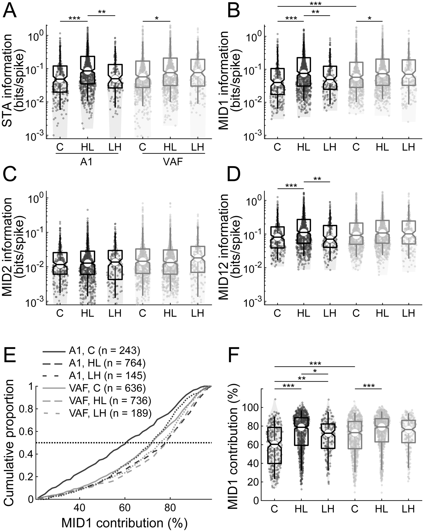
Information captured by single-filter and two-filter models for the noise-exposed and control animals in A1 and VAF.

(A-D) In A1, information values of STA (A), MID1 (B) and MID12 (D) increased with exposure to high-TMF-low-SMF-noise (HL, n = 764 neurons) compared to Control (C, n = 243) and low-TMF-high-SMF-noise-exposed (LH, n = 145) groups. A similar information increase for the HL group (n = 736 neurons) was observed in VAF for STA (A) and MID1 (B) but not for MID12 (D) compared to Control group (n = 636) while the increase did not significantly differ from LH group (n = 189). No significant difference was found among any groups and regions for MID2 (C). (E) Neurons from the Control group in A1 showed the lowest MID1 contribution. (F) MID1 contribution significantly increased for HL and LH animals in A1 and for HL animals in VAF. A1, black; VAF, grey. *, P < 0.05; **, P < 0.01; ***, P < 0.001.

Plasticity of filter interaction

We have shown for the unexposed Control group that the two filters interact more synergistically in A1 compared to VAF (Figure 2C–D). Next, we evaluated the change in information gain in the joint filter processing following noise exposure (Figure 8). In A1, the interaction of the two filters decreased for the HL and LH groups compared to the Control group (Figure 8A), while no difference was observed for VAF (Figure 8B). Statistical differences were found between Control and noise-exposed groups in A1 (KW, X² = 63.32, P < 0.001; post hoc, C vs. HL, P < 0.001; C vs. LH, P = 0.001) (Figure 8C). This observation demonstrates that the interaction between the two filters is affected by exposure-induced plasticity. While plasticity increased MID1 salience in A1, it reduced the interaction with the non-dominant second filter.

Figure 8.

Synergy decreased with noise exposure in A1 but not in VAF.

(A) In A1, neurons of the Control group had larger synergy than neurons of noise-exposed groups (HL and LH). (B) No significant difference was observed among the three groups in VAF. (C) Synergy decreased in A1 of HL and LH animals compared to Control animals. No significant difference was found in VAF. A1, black; VAF, grey. **, P < 0.01; ***, P < 0.001.

Plasticity of MID1 modulation transfer functions

We previously showed that modulation preferences captured by STA shifted away from the modulation parameters contained in the exposure noise statistics (Homma et al., 2020). Therefore, we hypothesized that MID1 would show shifts into the same direction as STA while MID2 may shift differently due to its limited preference overlap with the exposure noises and the independent nature of the two filters. We constructed population ripple transfer functions (pRTFs) for each experimental group and examined the changes in modulation preferences for MID1 and MID2, respectively (Figure 9 or 10). For evaluating the differences between Control and the two exposure groups, spectral and temporal modulation ranges of the pRTFs were divided into nine distinct sectors, which comprised the boundaries of the two exposed noises (Figures 9 and 10, see Methods).

Figure 9.

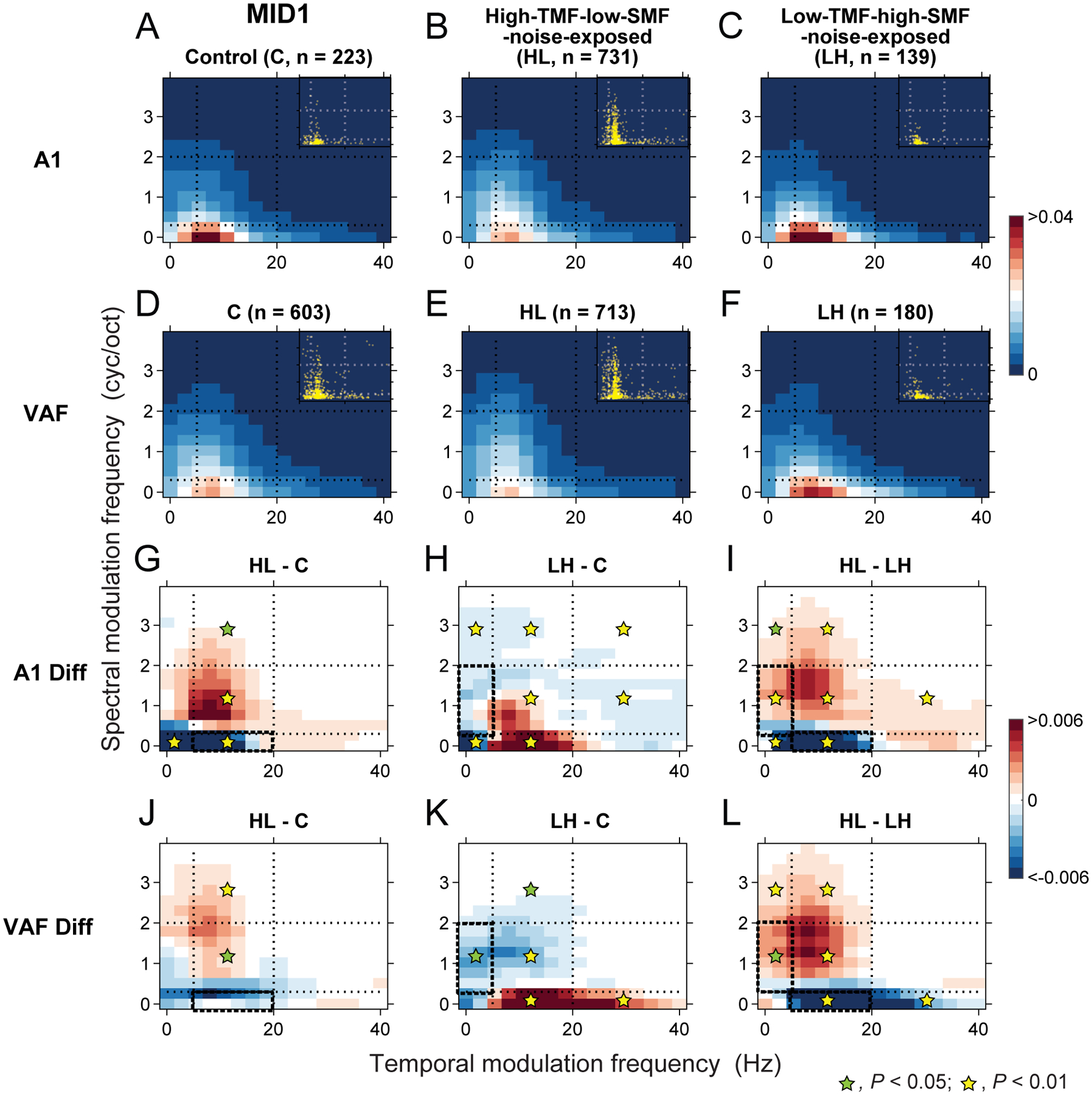
Noise-exposure modified ripple transfer function preferences of MID1.

(A-F) Population ripple transfer functions (pRTFs) of MID1 were obtained from A1 neurons for C (A), HL (B) and LH (C) animals as well as from VAF neurons for C (D), HL (E) and LH (F) animals. Color bar indicates normalized modulation power strength. Dotted lines indicate the boundaries of biased DMR noises. Insets indicate best temporal and spectral modulation frequencies of each neuron. (G-L) Differences of MID1 pRTFs between HL and C (G), between LH and C (H), and between HL and LH (I) groups for A1 and between HL and C (J), between LH and C (K), and between HL and LH (L) groups for VAF. Bold dashed boxes indicate the dominant modulation ranges of the exposure noises. Color bar indicates the values of differences. Noise exposure shifted the modulation preferences of MID1 away from the exposure noise statistics in A1 and VAF.

Figure 10.

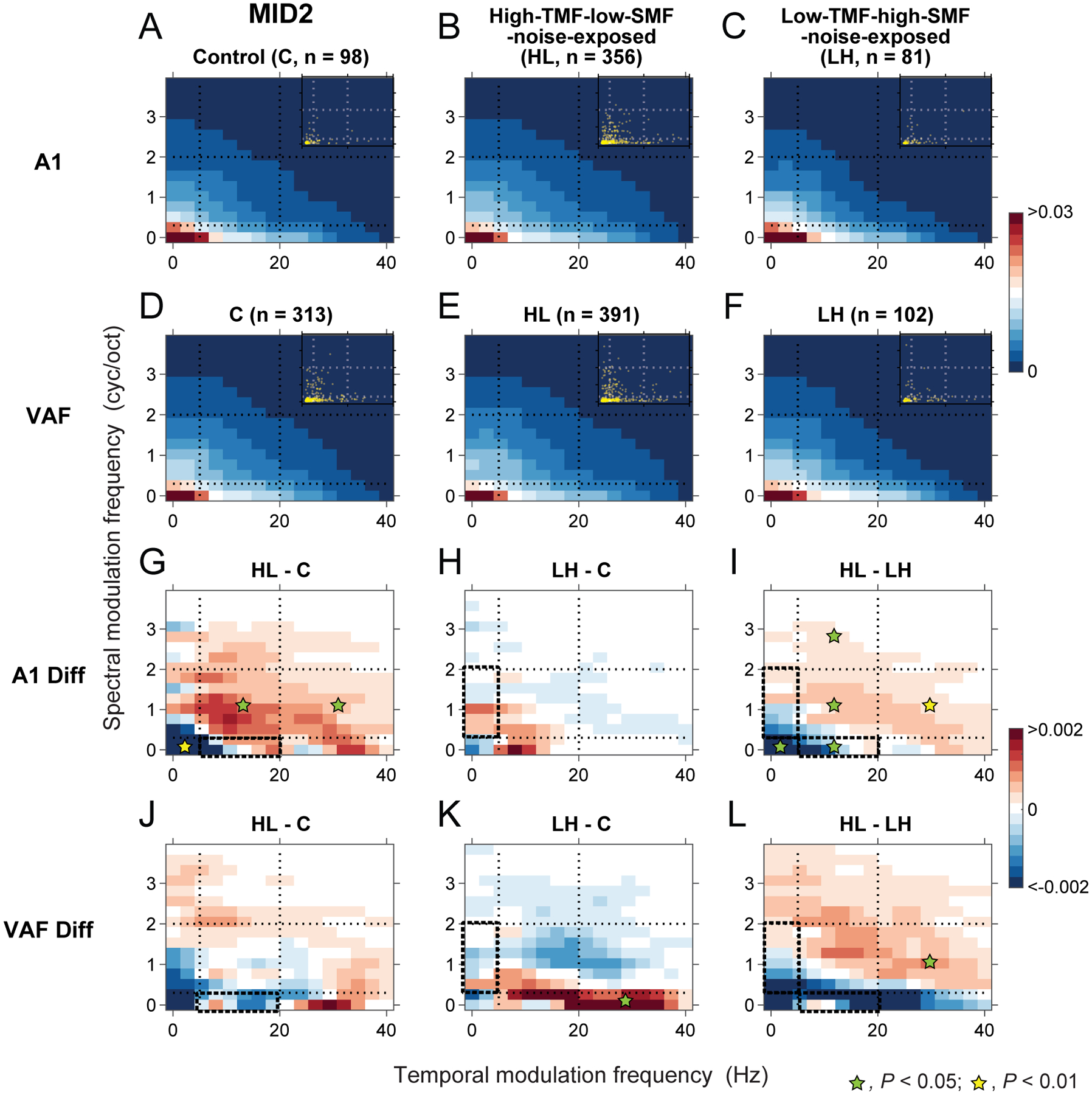
Noise-exposure only weakly modified ripple transfer function preferences of MID2.

The presentation scheme is the same as for Figure 9. (A-F) population ripple transfer functions (pRTFs) of MID2 were obtained for C (A), HL (B) and LH (C) animals of A1 and for C (D), HL (E) and LH (F) animals of VAF. (G-L) Differences of MID2 pRTFs were obtained between HL and C (G), between LH and C (H), and between HL and LH (I) groups for A1 and between HL and C (J), between LH and C (K), and between HL and LH (L) groups for VAF. MID2 modulation frequency preferences were lower than for MID1 both in A1 (A) and VAF (D) (see Figure 5). Modulation preference for MID2 shifted with noise exposure in the same direction as seen for MID1 although more diffusely and at a lower degree of significance.

The modulation preference of MID1 for the Control group in A1 (Figure 9A) showed a typical pattern of low temporal and spectral modulations. As expected, noise exposure induced specific changes for the preferred modulations (Figure 9B–C). Compared to the Control group, HL animals showed a reduced preference for lower spectral modulation frequencies present in the exposure noise and an increased preference for higher spectral modulation frequencies above the range contained in the exposure noise (Figure 9B). The difference of modulation preferences for the HL and Control animals reveals the reduction of modulation power to the exposure noise parameters (yellow asterisk in the bold dashed outline in Figure 9G; Bootstrap, P < 0.001; see Methods) including adjacent lower temporal modulation frequencies region with lower spectral modulation frequencies (yellow asterisk on blue region in Figure 9G; P < 0.001). In contrast, the modulation power associated with higher spectral modulation frequencies, not contained in the exposure noise, showed an increase (yellow or green asterisk on red region in Figure 9G; P < 0.04). Likewise, for the LH group, the difference between LH and Control groups showed a modulation power increase at lower temporal and spectral modulation frequencies outside the exposure range of spectral modulations (yellow asterisk on red region in Figure 9H, P < 0.001) with a decrease at the temporal modulation frequencies corresponding to the exposure noise and its surrounding parameter regions (yellow asterisks on blue region in Figure 9H; P < 0.01). This supports the interpretation that the representation of spectral modulation frequencies in the exposure noise decreased by noise rearing while that of the neighboring joint spectrotemporal modulations increased. The difference of modulation preferences between the two exposure conditions indicated contrasting, noise-specific effects for HL and LH groups (P < 0.03) (Figure 9I).

VAF neurons showed some similar plasticity effects. While the HL group did not significantly reduce the representation of spectral modulation frequencies contained in the exposed noise (blue in the bold dashed outline in Figure 9J; P > 0.05), it did increase power in the surrounding, unexposed spectral modulation ranges (asterisks on red region in Figure 9J; P < 0.03). This is consistent with the shift observed in A1 although the effect in VAF was smaller and toward higher spectral modulation frequencies potentially because the Control pRTF for VAF already had preference for higher spectral modulation frequencies than A1. By contrast, the LH group showed a clear reduction at the exposure noise modulations (green asterisk in the bold dashed outline in Figure 9K; P = 0.02). It also showed positive gain changes at higher temporal modulation frequencies combined with very low spectral modulation frequencies (asterisks on red region in Figure 9K; P < 0.005). The differences of modulation preferences between the HL and LH groups in VAF (Figure 9L) showed a similar pattern as for the contrast in A1 (Figure 9I). Although preferences between A1 and VAF for spectral modulation frequencies slightly differed, the noise-exposure effect for MID1 was consistent for both fields showing reduced representation for the exposed noise modulations and modulation power increases outside the exposed parameter ranges.

Plasticity of MID2 modulation transfer functions

Compared to MID1, the modulation preferences of MID2 were less variable between auditory fields or among groups (Figure 10; also see Figure 5). In particular, they showed preferences to very low temporal and spectral modulation frequencies consistent with the long-latency, broadly-tuned MID2 filter. Noise exposure parameters for the HL and the LH groups had only minor overlaps with the normal preference of MID2s. The exposure effects for MID2 in A1 were much smaller than seen for MID1, however, there was a similar trend. MID2 modulation preference shifts were also dependent on the environmental sound statistics. Similar to MID1, the HL group reduced the modulation power of MID2 at lower spectral modulation frequencies that were included in the exposure noise (yellow asterisk on blue region in Figure 10G; P = 0.007) and increased spectral modulation frequencies above the spectral modulation range of the exposure noise (green asterisks on red region in Figure 10G; P < 0.04). Similarly, as seen for MID1, LH group showed a tendency toward increased MID2 modulation power at lower spectral modulation frequencies, however, the changes did not reach statistical significance (Figure 10H). The contrast pattern seen in the difference of modulation preferences for the HL and LH groups supports the presence of exposure effects that depend on the noise statistics, mirroring those for MID1 (Figures 9I and 10I; P < 0.05).

For VAF, a similar trend was observed showing a decrease in modulation power contained in the exposure noise for the HL animals (Figure 10J, P > 0.05) and an increase at lower spectral modulation frequencies for the LH animals (asterisk on red region at higher temporal modulations in Figure 10K, P = 0.05). The difference of modulation preferences between the HL and LH groups also indicated that shifts in MID2 preferences were consistent with MID1 effects (asterisk on red region in Figure 10L, P = 0.03). We conclude that noise exposure similarly affects the structure of both multidimensional receptive field components but the extent was weak for the second filter, likely because the exposure noises were mostly outside the main modulation preferences of MID2.

Collectively, we showed that exposure plasticity increases the salience of the dominant first filter and decreases the synergy between the two filters in A1. In addition, noise-induced plasticity influences the structure of multidimensional spectrotemporal receptive fields by reducing responsiveness to the exposed background noise statistics similarly for both MIDs in the two core auditory fields although the effect was more limited for the second filter.

DISCUSSION

The goal of this study was to identify the functional organization of multidimensional RFs in rat core auditory cortex and to determine its plasticity in response to the exposure to different background sounds. We first characterized mutual information values and modulation preferences of the two main filters, MID1 and MID2, that emerge when applying an information-based dimensionality reduction technique (Sharpee et al., 2004; Atencio et al., 2008). We then compared the functional properties and the interactions of the two filters between the two major core auditory fields, A1 and VAF. We found that VAF has higher temporal and spectral modulation preferences, higher information values for the first filter (MID1), and a lower interaction strength of the two filters compared to A1. This suggests that VAF likely performs a more linear signal analysis than A1. When expanding the comparison to animals that were exposed to different modulated background noises at young age, we found that the experience altered RF structures of both MID filters in similar ways in both auditory fields, although to a lesser degree for MID2. In addition, plasticity increased the strength of the first filter but reduced the synergy between the two filters in A1. These results highlight that i) the two filters encode distinctly different stimulus domains, both in A1 and VAF, ii) MID1 differs between the two fields functionally and in strength, iii), plastic changes of salience and filter interactions differ between the two fields and iv) congruent plastic changes can affect the functional structure of the two filters in both fields. Taken together, this suggests that core fields not only differ in what they process but also how they weigh the information provided by the two filter components. Furthermore, plasticity effects predominately enhance the ability to process sounds, either by enhancing the representation of meaningful sounds or reducing the representation of meaningless or interfering sounds.

Approach:

MID analysis is a productive approach for estimating multidimensional RFs based on information theory (Sharpee et al., 2004). Although a single spectrotemporal feature can provide important insights for auditory cortical processing (Blake and Merzenich, 2002; Elhilali et al., 2004; Gourevitch et al., 2009), recent studies showed that many auditory cortical neurons can encode more than one stimulus feature (Atencio et al., 2008; Sharpee et al., 2011; Harper et al., 2016; Kozlov and Gentner, 2016; Atencio and Sharpee, 2017; Shih et al., 2020). The MID method is a model that can capture some aspects of nonlinear processing by neurons and is not limited by stimulus structures (Simoncelli et al., 2004; Schwartz et al., 2006). Our rat A1 data paralleled data from cat A1 neurons (Atencio et al., 2008; Shih et al., 2020) with regard to the expression of at least two interacting RFs per neuron. We further showed that environmental manipulation can alter structure, salience, and interactions of the two MID filters. Our results support that MID analysis can, at a minimum, capture biological functional changes of the auditory RFs.

Auditory cortical field differences:

Mammalian auditory cortex has distinct field organizations (Budinger et al., 2000; Wallace et al., 2000; Bendor and Wang, 2008; Lee and Winer, 2008; Hackett, 2011; Bizley et al., 2015). In rat, at least five distinct cortical fields have been identified, and the physiological and anatomical differences suggest parallel processing at A1 and VAF as each receives distinctive thalamocortical inputs (Kimura et al., 2003; Rutkowski et al., 2003; Polley et al., 2007; Storace et al., 2010, 2011; Smith et al., 2012). We observed shorter latencies in A1 and narrower tuning in VAF comparable to previous, single filter studies showing somewhat different temporal and spectral resolutions of each field (Polley et al., 2007; Lee et al., 2016; Osman et al., 2018). In particular, we showed that VAF had higher temporal and spectral modulation preferences and higher information values for the first, dominant filter. In cat, A1 comprises iso-frequency bands receiving non-overlapping thalamic inputs organized in the caudal-to-rostral dimension, with narrowly tuned neurons showing higher spectral modulation preferences and feature selectivity compared to the broadly tuned neurons (Calford, 1983; Rodrigues-Dagaeff et al., 1989; Rouiller et al., 1989; Read et al., 2001, 2011; Atencio and Schreiner, 2012). A similar anatomical organization has been observed in rats with A1 and VAF receiving parallel projections from the lemniscal thalamus (Polley et al., 2007; Storace et al., 2010, 2011) as well as for other species (gerbil: Saldeitis et al. 2014; guinea pig: Redies et al. 1989; marmoset: De La Mothe et al. 2006; mouse: Hackett et al. 2011; rabbit: Cetas et al. 2001; Velenovsky et al. 2003). The observed physiological differences between A1 and VAF suggest that these might be analogous to those observed for the broadly and narrowly tuned iso-frequency regions of cat A1.

Rat A1 neurons exhibited a stronger interaction of the two filters compared to VAF. We previously showed that the contribution of the second filter increased from midbrain and thalamus to cortex in the ascending auditory pathway, suggesting that thalamocortical and corticocortical convergence increases multi-feature sensitivity and synergy (Atencio et al., 2012; Shih et al., 2020). The convergence of parallel thalamic inputs seems to differ between A1 and VAF as broadly tuned neurons receive more variable thalamocortical (Read et al., 2011; Saldeitis et al., 2014) or corticocortical (K. Imaizumi, personnel communication) projections across frequencies. This supports our finding of broader spectral tuning and larger synergy for A1 compared to VAF although synergy is not explained by spectral integration alone (see below).

The systematic difference in the modulation domain captured by the two filters suggests that cortical, but not subcortical, neurons can directly exploit stimulus-specific interactions between different components of the auditory scene. This could reveal relevant aspects for cortical sound processing, e.g., for the analysis of certain foreground sounds, like vocalizations, in the presence of different background conditions. An additional perspective arises from the observation that the filter properties seen for MID2 in these core fields appears to be very similar to the dominant stimulus domain of MID1 in higher auditory fields in humans (Hullett et al., 2016). The interpretation of the potential role of those filter properties in higher areas has focused on the role of suprasegmental influences in speech processing. The potential transformation of these different stimulus aspects and their interactions through the cortical hierarchy, however, requires further attention.

Exposure-induced receptive field plasticity:

We initially had hypothesized that noise exposure may shift spectrotemporal preferences of MID1 and MID2 into different directions since the two filters are independent of each other and may serve different purposes. We found, however, that noise exposure altered the RF structures of the two filters in a similar manner. While sound exposure to specific signals or enriched auditory environments mainly resulted in over-representation of the presented sound features (Zhang et al., 2002; de Villers-Sidani et al., 2007; Grécová et al., 2009; Insanally et al., 2009; Bao et al., 2013; Pysanenko et al., 2018), we showed that continuous broadband noise exposure can suppress the responsiveness to noise parameters leading to a better signal-to-noise ratio at the neuronal and behavioral level (Homma et al., 2020). This shift in sound preference was similar to a suppression of CFs falling within the range of a band-limited exposure noise and an enhancement of CFs at the edges of such a noise (Noreña et al., 2006; Pienkowski and Eggermont, 2009; Pienkowski et al., 2011). Reduced firing rates have also been observed for an exposure stimulus with two correlated features (Lu et al., 2019). In the present study, we found that the first filter, MID1, shifted its modulation preferences to effectively avoid the exposed sound statistics similar to what had been observed for STA. Additionally, although the effect was much weaker than for MID1, we observed that the second filter, MID2, also altered its modulation preferences in the same general direction as the first filter. The plasticity effects were somewhat field-specific. The HL group, exposed to lower spectral modulation frequencies, showed strong preference shifts to higher spectral modulation frequencies in A1. For the LH group, exposed to higher spectral modulation frequencies, an opposite shift to lower spectral modulation frequencies was observed in VAF. These field-specific functional changes suggest that expression of plasticity depends on the relevance attached to the signal, its sound structure, and the original properties of the filters. The particular condition utilized in the present study was the presence of moderately loud background sound, which itself carries no useful information but interferes with the processing of some meaningful foreground sounds without severely preventing the perception of vocalizations from the mother or other pups. The plasticity to this sound exposure resulted in a more favorable processing condition by reducing responses to the background sounds and, therefore, enhancing the signal-in-noise ratio for individual neurons (Homma et al., 2020). Behaviorally-induced plasticity is widely distributed in the auditory cortex (Centanni et al., 2013; Engineer et al., 2015) and can result in enhancement as well as in reduction of certain sound parameter representation (Noreña et al., 2006; de Villers-Sidani and Merzenich, 2011). Our results demonstrate that both auditory cortical fields have the ability of adopting the structure and interaction of the first and second filters that minimize potential adverse noise interference on signal processing.

Synergy:

We examined if noise exposure alters the information conveyed by the two filters and if the changes affect the interaction of the two filters. Our results showed that noise exposure reduced the synergy of the two filters compared to the unexposed animals. Since A1 showed larger synergy values than VAF in the Control group, the exposure effect was stronger in A1. In A1, the information values of MID1 and MID12 increased for the noise-exposed group while the information values of MID2 did not differ from the Control group. The gain of the joint filter processing (the differences between MID1 and MID12) was largest in the Control group (Figure 7E–F). Thus, the decreased synergy for exposed animals reflected an increased feature selectivity of the first filter and a decreased relative MID2 contribution. Exposure to moderately loud modulated noise improved the ability of animals to discriminate rat vocalizations from background noise (Homma et al., 2020). Enhanced selectivity in the first filter, which can be thought of as a detector of dominant foreground features (Atencio et al., 2008, 2009, 2012), appears to have achieved better signal-in-noise processing for the noise-exposed animals. The second filter has been shown to play a role in adapting to sound environments with higher variance (Sharpee et al., 2011). One of the confounds in our exposure paradigm was overtraining of the animals to the exposure noise stimulus. If the role of the second filter is to assist novelty detection or to encode context dependency, the overtraining may have improved feature detection and reduced the ability of the second filter to perform its roles. The second filter may be more important in ecological sound processing, because in real life, the environment comprises a variety of different, changing complex sounds (McDermott and Simoncelli, 2011), in which primary auditory tasks, like signal detection and discrimination, have to take place. Finally, one can speculate that if reduction of synergy is of advantage when challenged with statistically predictable background sounds, increased synergy may be expected when faced with the analysis of statistically unpredictable, complex sound feature constellations or contexts.

Emergence of two-filter RF:

It is noteworthy that the synergy in rat auditory cortex was comparable to cat auditory cortex while subcortical stations had little gain from two-filter models (Atencio et al., 2008, 2012; Shih et al., 2020). Even with a reduced synergy for the exposed animals, it still showed some benefit of the additional second filter compared to that seen in subcortical stations. Thus, these data suggest that the transformation from thalamus to cortex combined with influences of corticocortical processing are key contributors to generate multi-filter RFs. While we do not know the exact hierarchical order of A1 and VAF in rat, VAF has been considered to be hierarchically close but slightly higher than A1 (Lee et al., 2016; Osman et al., 2018). Additionally, these two pathways may be independent with different excitatory and inhibitory balance (Read et al., 2001; Yuan et al., 2011). As discussed above, rat A1 and VAF receive parallel thalamocortical inputs from the ventral division of the medial geniculate body (Polley et al., 2007; Storace et al., 2010, 2011). Since our exposure was likely to include the auditory critical period during which thalamocortical axons mature and develop tonotopy in A1 (Zhao et al., 2009; Barkat et al., 2011; Takesian et al., 2018), we cannot exclude the possibility that fundamental local connectivity may have been altered during noise exposure. Our exposure DMR, however, was broadband noise with coherent temporal and spectral structures (Escabi and Schreiner, 2002) and did not appear to alter cortical tonotopic organization like seen for pure tone exposure (Zhang et al., 2001; de Villers-Sidani et al., 2007; Han et al., 2007; Insanally et al., 2009). Therefore, we postulate that changes in synaptic strength of converging inputs altered synergy as well as modulation preferences for the exposed animals (Wehr and Zador, 2003; Froemke et al., 2007; Speechley et al., 2007; Dorrn et al., 2010; Sun et al., 2010; Cai et al., 2018). Furthermore, we expect that synergy may be larger in the awake condition since top-down modulation and/or attentional effects are lacking under anesthesia. It will be essential to examine multidimensional RFs in the un-anesthetized preparation and in animals engaged in a behavioral task.

In the present study, we first characterized the functional organization of rat A1 and VAF based on the multidimensional RFs revealing distinct functional properties of the two filters. Then, we showed that exposure-induced plasticity reduced the interaction between the two filters in A1. Early noise exposure similarly affected the structure of the first and second RF dimension for both fields dependent on the environmental noise statistics. These findings highlight field differences among core cortical fields and showed that plasticity can affect both the content of the multidimensional RFs as well as their potential for cooperative processing.

ABBREVIATIONS

A1

primary auditory cortex

BW

bandwidth

CF

characteristic frequency

DMR

dynamic moving ripple

HL

high-TMF-low-SMF-noise-exposed

KS

Kolmogorov-Smirnov

KW

Kruskal-Wallis

LH

low-TMF-high-SMF-noise-exposed

MID

maximally informative dimension

pRTF

population ripple transfer function

Q

quality factor (CF/BW)

RF

receptive field

r_s

Spearman’s rho

RTF

ripple transfer function

SMF

spectral modulation frequency

STA

spike-triggered average

STRF

spectrotemporal receptive field

TMF

temporal modulation frequency

VAF

ventral auditory field

REFERENCES

- Aertsen AM, Johannesma PI (1981) The spectro-temporal receptive field. A functional characteristic of auditory neurons. Biol Cybern 42:133–143 Available at: http://www.ncbi.nlm.nih.gov/pubmed/7326288. [DOI] [PubMed] [Google Scholar]
- Agüera y Arcas B, Fairhall AL, Bialek W (2003) Computation in a single neuron: Hodgkin and Huxley revisited. Neural Comput 15:1715–1749 Available at: https://www.princeton.edu/~wbialek/our_papers/aguerayarcas+al_03.pdf. [DOI] [PubMed] [Google Scholar]
- Atencio CA, Schreiner CE (2010) Laminar diversity of dynamic sound processing in cat primary auditory cortex. J Neurophysiol 103:192–205 Available at: http://www.ncbi.nlm.nih.gov/pubmed/19864440. [DOI] [PMC free article] [PubMed] [Google Scholar]
- Atencio CA, Schreiner CE (2012) Spectrotemporal processing in spectral tuning modules of cat primary auditory cortex. PLoS One 7:e31537 Available at: http://www.ncbi.nlm.nih.gov/pubmed/22384036. [DOI] [PMC free article] [PubMed] [Google Scholar]
- Atencio CA, Schreiner CE (2016) Functional congruity in local auditory cortical microcircuits. Neuroscience 316:402–419 Available at: http://linkinghub.elsevier.com/retrieve/pii/S0306452216000063. [DOI] [PMC free article] [PubMed] [Google Scholar]
- Atencio CA, Sharpee TO (2017) Multidimensional receptive field processing by cat primary auditory cortical neurons. Neuroscience 359:130–141 Available at: 10.1016/j.neuroscience.2017.07.003. [DOI] [PMC free article] [PubMed] [Google Scholar]
- Atencio CA, Sharpee TO, Schreiner CE (2008) Cooperative nonlinearities in auditory cortical neurons. Neuron 58:956–966 Available at: http://www.ncbi.nlm.nih.gov/pubmed/18579084. [DOI] [PMC free article] [PubMed] [Google Scholar]
- Atencio CA, Sharpee TO, Schreiner CE (2009) Hierarchical computation in the canonical auditory cortical circuit. Proc Natl Acad Sci U S A 106:21894–21899 Available at: http://eutils.ncbi.nlm.nih.gov/entrez/eutils/elink.fcgi?dbfrom=pubmed&id=19918079&retmode=ref&cmd=prlinks%5Cnpapers3://publication/doi/10.1073/pnas.0908383106. [DOI] [PMC free article] [PubMed] [Google Scholar]
- Atencio CA, Sharpee TO, Schreiner CE (2012) Receptive field dimensionality increases from the auditory midbrain to cortex. J Neurophysiol 107:2594–2603 Available at: http://www.ncbi.nlm.nih.gov/entrez/query.fcgi?cmd=Retrieve&db=pubmed&dopt=AbstractPlus&list_uids=22323634. [DOI] [PMC free article] [PubMed] [Google Scholar]
- Bao S, Chang EF, Teng C-L, Heiser MA, Merzenich MM (2013) Emergent categorical representation of natural, complex sounds resulting from the early post-natal sound environment. Neuroscience 248:30–42 Available at: http://www.ncbi.nlm.nih.gov/pubmed/11264676. [DOI] [PMC free article] [PubMed] [Google Scholar]
- Barkat TR, Polley DB, Hensch TK (2011) A critical period for auditory thalamocortical connectivity. Nat Neurosci 14:1189–1194 Available at: http://www.pubmedcentral.nih.gov/articlerender.fcgi?artid=3419581&tool=pmcentrez&rendertype=abstract [Accessed May 28, 2013]. [DOI] [PMC free article] [PubMed] [Google Scholar]
- Bendor D, Wang X (2008) Neural response properties of primary, rostral, and rostrotemporal core fields in the auditory cortex of marmoset monkeys. J Neurophysiol 100:888–906. [DOI] [PMC free article] [PubMed] [Google Scholar]
- Bizley JK, Bajo VM, Nodal FR, King AJ (2015) Cortico-cortical connectivity within ferret auditory cortex. J Comp Neurol 000:000–000 Available at: http://doi.wiley.com/10.1002/cne.23784. [DOI] [PMC free article] [PubMed] [Google Scholar]
- Blake DT, Merzenich MM (2002) Changes of AI receptive fields with sound density. J Neurophysiol 88:3409–3420 Available at: http://jn.physiology.org/cgi/doi/10.1152/jn.00233.2002. [DOI] [PubMed] [Google Scholar]
- Budinger E, Heil P, Scheich H (2000) Functional organization of auditory cortex in the Mongolian gerbil (Meriones unguiculatus). III. Anatomical subdivisions and corticocortical connections. Eur J Neurosci 12:2425–2451. [DOI] [PubMed] [Google Scholar]
- Cai D, Han R, Liu M, Xie F, You L, Zheng Y, Zhao L, Yao J, Wang Y, Yue Y, Schreiner CE, Yuan K (2018) A Critical Role of Inhibition in Temporal Processing Maturation in the Primary Auditory Cortex. Cereb Cortex 28:1610–1624 Available at: http://www.ncbi.nlm.nih.gov/pubmed/28334383. [DOI] [PMC free article] [PubMed] [Google Scholar]
- Calford MB (1983) The parcellation of the medial geniculate body of the cat defined by the auditory response properties of single units. J Neurosci 3:2350–2364. [DOI] [PMC free article] [PubMed] [Google Scholar]
- Centanni TM, Engineer CT, Kilgard MP (2013) Cortical speech-evoked response patterns in multiple auditory fields are correlated with behavioral discrimination ability. J Neurophysiol 110:177–189 Available at: http://www.physiology.org/doi/10.1152/jn.00092.2013. [DOI] [PMC free article] [PubMed] [Google Scholar]
- Cetas JS, Price RO, Velenovsky DS, Sinex DG, McMullen NT (2001) Frequency organization and cellular lamination in the medial geniculate body of the rabbit. Hear Res 155:113–123 Available at: http://www.ncbi.nlm.nih.gov/pubmed/11335081. [DOI] [PubMed] [Google Scholar]
- Chang EF, Merzenich MM (2003) Environmental noise retards auditory cortical development. Science 300:498–502 Available at: http://www.ncbi.nlm.nih.gov/pubmed/12702879. [DOI] [PubMed] [Google Scholar]
- Chung JE, Magland JF, Barnett AH, Tolosa VM, Tooker AC, Lee KY, Shah KG, Felix SH, Frank LM, Greengard LF (2017) A Fully Automated Approach to Spike Sorting. Neuron 95:1381–1394.e6 Available at: 10.1016/j.neuron.2017.08.030. [DOI] [PMC free article] [PubMed] [Google Scholar]
- de Boer R, Kuyper P (1968) Triggered correlation. IEEE Trans Biomed Eng 15:169–179 Available at: http://www.ncbi.nlm.nih.gov/pubmed/5667803. [DOI] [PubMed] [Google Scholar]
- De La Mothe LA, Blumell S, Kajikawa Y, Hackett TA (2006) Thalamic connections of the auditory cortex in marmoset monkeys: Core and medial belt regions. J Comp Neurol 496:72–96 Available at: http://doi.wiley.com/10.1002/cne.20924. [DOI] [PMC free article] [PubMed] [Google Scholar]
- de Ruyter van Steveninck R, Bialek W (1988) Real-time performance of a movement-sensitive neuron in the blowfly visual system: coding and information transfer in short spike sequences. Proc R Soc London Ser B Biol Sci 234:379–414 Available at: http://www.royalsocietypublishing.org/doi/10.1098/rspb.1988.0055. [Google Scholar]
- de Villers-Sidani E, Chang EF, Bao S, Merzenich MM (2007) Critical period window for spectral tuning defined in the primary auditory cortex (A1) in the rat. J Neurosci 27:180–189 Available at: http://www.jneurosci.org/cgi/doi/10.1523/JNEUROSCI.3227-06.2007. [DOI] [PMC free article] [PubMed] [Google Scholar]
- de Villers-Sidani E, Merzenich MM (2011) Lifelong plasticity in the rat auditory cortex: basic mechanisms and role of sensory experience. Prog Brain Res 191:119–131 Available at: 10.1016/B978-0-444-53752-2.00009-6. [DOI] [PubMed] [Google Scholar]
- DeCharms RC, Blake DT, Merzenich MM (1998) Optimizing sound features for cortical neurons. Science 280:1439–1443 Available at: http://www.ncbi.nlm.nih.gov/pubmed/9603734. [DOI] [PubMed] [Google Scholar]
- Depireux DA, Simon JZ, Klein DJ, Shamma SA (2001) Spectro-temporal response field characterization with dynamic ripples in ferret primary auditory cortex. J Neurophysiol 85:1220–1234 Available at: http://www.ncbi.nlm.nih.gov/pubmed/11247991. [DOI] [PubMed] [Google Scholar]
- Dorrn AL, Yuan K, Barker AJ, Schreiner CE, Froemke RC (2010) Developmental sensory experience balances cortical excitation and inhibition. Nature 465:932–936 Available at: 10.1038/nature09119. [DOI] [PMC free article] [PubMed] [Google Scholar]
- Elhilali M, Fritz JB, Klein DJ, Simon JZ, Shamma SA (2004) Dynamics of precise spike timing in primary auditory cortex. J Neurosci 24:1159–1172 Available at: http://www.jneurosci.org/cgi/doi/10.1523/JNEUROSCI.3825-03.2004. [DOI] [PMC free article] [PubMed] [Google Scholar]
- Engineer CT, Rahebi KC, Buell EP, Fink MK, Kilgard MP (2015) Speech training alters consonant and vowel responses in multiple auditory cortex fields. Behav Brain Res 287:256–264 Available at: 10.1016/j.bbr.2015.03.044. [DOI] [PMC free article] [PubMed] [Google Scholar]
- Escabí MA, Read HL, Viventi J, Kim D-H, Higgins NC, Storace DA, Liu ASK, Gifford AM, Burke JF, Campisi M, Kim Y-S, Avrin AE, Spiegel Jan V der, Huang Y, Li M, Wu J, Rogers JA, Litt B, Cohen YE (2014) A high-density, high-channel count, multiplexed μECoG array for auditory-cortex recordings. J Neurophysiol 112:1566–1583 Available at: http://www.ncbi.nlm.nih.gov/pubmed/24920021. [DOI] [PMC free article] [PubMed] [Google Scholar]
- Escabi MA, Schreiner CE (2002) Nonlinear spectrotemporal sound analysis by neurons in the auditory midbrain. J Neurosci 22:4114–4131. [DOI] [PMC free article] [PubMed] [Google Scholar]
- Fritz JB, Elhilali M, David SV., Shamma SA (2007) Does attention play a role in dynamic receptive field adaptation to changing acoustic salience in A1? Hear Res 229:186–203. [DOI] [PMC free article] [PubMed] [Google Scholar]
- Froemke RC, Merzenich MM, Schreiner CE (2007) A synaptic memory trace for cortical receptive field plasticity. Nature 450:425–429 Available at: 10.1038/nature06289. [DOI] [PubMed] [Google Scholar]
- Froemke RC, Schreiner CE (2015) Synaptic plasticity as a cortical coding scheme. Curr Opin Neurobiol 35:185–199 Available at: 10.1016/j.conb.2015.10.003. [DOI] [PMC free article] [PubMed] [Google Scholar]
- Gourévitch B, Noreña A, Shaw G, Eggermont JJ (2009) Spectrotemporal receptive fields in anesthetized cat primary auditory cortex are context dependent. Cereb Cortex 19:1448–1461 Available at: http://www.ncbi.nlm.nih.gov/pubmed/18854580. [DOI] [PubMed] [Google Scholar]
- Grécová J, Bures Z, Popelár J, Suta D, Syka J (2009) Brief exposure of juvenile rats to noise impairs the development of the response properties of inferior colliculus neurons. Eur J Neurosci 29:1921–1930 Available at: http://www.ncbi.nlm.nih.gov/pubmed/19473244. [DOI] [PubMed] [Google Scholar]
- Hackett TA (2011) Information flow in the auditory cortical network. Hear Res 271:133–146. [DOI] [PMC free article] [PubMed] [Google Scholar]
- Hackett TA, Barkat TR, O’Brien BMJ, Hensch TK, Polley DB (2011) Linking topography to tonotopy in the mouse auditory thalamocortical circuit. J Neurosci 31:2983–2995 Available at: http://www.pubmedcentral.nih.gov/articlerender.fcgi?artid=3073837&tool=pmcentrez&rendertype=abstract [Accessed May 24, 2013]. [DOI] [PMC free article] [PubMed] [Google Scholar]
- Han YK, Köver H, Insanally MN, Semerdjian JH, Bao S (2007) Early experience impairs perceptual discrimination. Nat Neurosci 10:1191–1197 Available at: http://www.ncbi.nlm.nih.gov/pubmed/17660815. [DOI] [PubMed] [Google Scholar]
- Harper NS, Schoppe O, Willmore BDB, Cui Z, Schnupp JWH, King AJ (2016) Network Receptive Field Modeling Reveals Extensive Integration and Multi-feature Selectivity in Auditory Cortical Neurons. PLoS Comput Biol 12:e1005113 Available at: http://dx.plos.org/10.1371/journal.pcbi.1005113. [DOI] [PMC free article] [PubMed] [Google Scholar]
- Homma NY, Hullett PW, Atencio CA, Schreiner CE (2020) Auditory Cortical Plasticity Dependent on Environmental Noise Statistics. Cell Rep 30:4445–4458.e5 Available at: 10.1016/j.celrep.2020.03.014. [DOI] [PMC free article] [PubMed] [Google Scholar]
- Hullett PW, Hamilton LS, Mesgarani N, Schreiner CE, Chang EF (2016) Human Superior Temporal Gyrus Organization of Spectrotemporal Modulation Tuning Derived from Speech Stimuli. J Neurosci 36:2014–2026 Available at: http://www.ncbi.nlm.nih.gov/pubmed/26865624%5Cnhttp://www.pubmedcentral.nih.gov/articlerender.fcgi?artid=PMC4748082. [DOI] [PMC free article] [PubMed] [Google Scholar]
- Insanally MN, Köver H, Kim H, Bao S (2009) Feature-dependent sensitive periods in the development of complex sound representation. J Neurosci 29:5456–5462 Available at: http://www.pubmedcentral.nih.gov/articlerender.fcgi?artid=2717948&tool=pmcentrez&rendertype=abstract. [DOI] [PMC free article] [PubMed] [Google Scholar]
- Kimura A, Donishi T, Sakoda T, Hazama M, Tamai Y (2003) Auditory thalamic nuclei projections to the temporal cortex in the rat. Neuroscience 117:1003–1016 Available at: http://www.ncbi.nlm.nih.gov/pubmed/12654352. [DOI] [PubMed] [Google Scholar]
- Kozlov AS, Gentner TQ (2016) Central auditory neurons have composite receptive fields. Proc Natl Acad Sci U S A 113:1441–1446 Available at: http://www.ncbi.nlm.nih.gov/pubmed/26787894. [DOI] [PMC free article] [PubMed] [Google Scholar]
- Lee CC, Winer JA (2008) Connections of cat auditory cortex: II. Commissural system. J Comp Neurol 507:1901–1919 Available at: http://www.pubmedcentral.nih.gov/articlerender.fcgi?artid=2678022&tool=pmcentrez&rendertype=abstract. [DOI] [PMC free article] [PubMed] [Google Scholar]
- Lee CM, Osman AF, Volgushev M, Escabí MA, Read HL (2016) Neural spike-timing patterns vary with sound shape and periodicity in three auditory cortical fields. J Neurophysiol 115:1886–1904 Available at: http://www.physiology.org/doi/10.1152/jn.00784.2015. [DOI] [PMC free article] [PubMed] [Google Scholar]
- Lu K, Liu W, Dutta K, Zan P, Fritz JB, Shamma SA (2019) Adaptive Efficient Coding of Correlated Acoustic Properties. J Neurosci 39:8664–8678 Available at: http://www.jneurosci.org/lookup/doi/10.1523/JNEUROSCI.0141-19.2019. [DOI] [PMC free article] [PubMed] [Google Scholar]
- Machens CK, Wehr MS, Zador AM (2004) Linearity of cortical receptive fields measured with natural sounds. J Neurosci 24:1089–1100 Available at: http://www.ncbi.nlm.nih.gov/pubmed/14762127. [DOI] [PMC free article] [PubMed] [Google Scholar]
- Marmarelis VZ (1997) Modeling methodology for nonlinear physiological systems. Ann Biomed Eng 25:239–251 Available at: http://www.ncbi.nlm.nih.gov/pubmed/9084829. [DOI] [PubMed] [Google Scholar]
- McDermott JH, Simoncelli EP (2011) Sound texture perception via statistics of the auditory periphery: evidence from sound synthesis. Neuron 71:926–940 Available at: 10.1016/j.neuron.2011.06.032. [DOI] [PMC free article] [PubMed] [Google Scholar]
- Meyer AF, Williamson RS, Linden JF, Sahani M (2016) Models of Neuronal Stimulus-Response Functions: Elaboration, Estimation, and Evaluation. Front Syst Neurosci 10:109 Available at: http://www.ncbi.nlm.nih.gov/pubmed/28127278. [DOI] [PMC free article] [PubMed] [Google Scholar]
- Nieto-Diego J, Malmierca MS (2016) Topographic Distribution of Stimulus-Specific Adaptation across Auditory Cortical Fields in the Anesthetized Rat. PLoS Biol 14:1–30. [DOI] [PMC free article] [PubMed] [Google Scholar]
- Noreña AJ, Gourévitch B, Aizawa N, Eggermont JJ (2006) Spectrally enhanced acoustic environment disrupts frequency representation in cat auditory cortex. Nat Neurosci 9:932–939 Available at: http://www.ncbi.nlm.nih.gov/pubmed/16783369. [DOI] [PubMed] [Google Scholar]
- Oliver DL, Izquierdo MA, Malmierca MS (2011) Persistent effects of early augmented acoustic environment on the auditory brainstem. Neuroscience 184:75–87 Available at: http://www.ncbi.nlm.nih.gov/pubmed/21496479. [DOI] [PMC free article] [PubMed] [Google Scholar]
- Osman AF, Lee CM, Escabí MA, Read HL (2018) A Hierarchy of Time Scales for Discriminating and Classifying the Temporal Shape of Sound in Three Auditory Cortical Fields. J Neurosci 38:6967–6982 Available at: http://www.jneurosci.org/lookup/doi/10.1523/JNEUROSCI.2871-17.2018. [DOI] [PMC free article] [PubMed] [Google Scholar]
- Osmanski MS, Wang X (2015) Behavioral dependence of auditory cortical responses. Brain Topogr 28:365–378 Available at: http://www.ncbi.nlm.nih.gov/pubmed/25690831. [DOI] [PMC free article] [PubMed] [Google Scholar]
- Pienkowski M, Eggermont JJ (2009) Long-term, partially-reversible reorganization of frequency tuning in mature cat primary auditory cortex can be induced by passive exposure to moderate-level sounds. Hear Res 257:24–40 Available at: 10.1016/j.heares.2009.07.011. [DOI] [PubMed] [Google Scholar]
- Pienkowski M, Munguia R, Eggermont JJ (2011) Passive exposure of adult cats to bandlimited tone pip ensembles or noise leads to long-term response suppression in auditory cortex. Hear Res 277:117–126 Available at: 10.1016/j.heares.2011.02.002. [DOI] [PubMed] [Google Scholar]
- Polley DB, Read HL, Storace DA, Merzenich MM (2007) Multiparametric auditory receptive field organization across five cortical fields in the albino rat. J Neurophysiol 97:3621–3638 Available at: http://www.ncbi.nlm.nih.gov/pubmed/17376842. [DOI] [PubMed] [Google Scholar]
- Pysanenko K, Bureš Z, Lindovský J, Syka J (2018) The Effect of Complex Acoustic Environment during Early Development on the Responses of Auditory Cortex Neurons in Rats. Neuroscience 371:221–228 Available at: https://linkinghub.elsevier.com/retrieve/pii/S0306452217308667. [DOI] [PubMed] [Google Scholar]
- Rahman M, Willmore BDB, King AJ, Harper NS (2019) A dynamic network model of temporal receptive fields in primary auditory cortex. PLoS Comput Biol 15:e1006618 Available at: http://www.ncbi.nlm.nih.gov/pubmed/31059503. [DOI] [PMC free article] [PubMed] [Google Scholar]
- Read HL, Nauen DW, Escabi MA, Miller LM, Schreiner CE, Winer JA (2011) Distinct core thalamocortical pathways to central and dorsal primary auditory cortex. Hear Res 274:95–104 Available at: http://eutils.ncbi.nlm.nih.gov/entrez/eutils/elink.fcgi?dbfrom=pubmed&id=21145383&retmode=ref&cmd=prlinks%5Cnpapers3://publication/doi/10.1016/j.heares.2010.11.010. [DOI] [PMC free article] [PubMed] [Google Scholar]
- Read HL, Winer JA, Schreiner CE (2001) Modular organization of intrinsic connections associated with spectral tuning in cat auditory cortex. Proc Natl Acad Sci U S A 98:8042–8047 Available at: http://www.ncbi.nlm.nih.gov/pubmed/11438747. [DOI] [PMC free article] [PubMed] [Google Scholar]
- Redies H, Sieben U, Creutzfeldt OD (1989) Functional subdivisions in the auditory cortex of the guinea pig. J Comp Neurol 282:473–488 Available at: http://doi.wiley.com/10.1002/cne.902820402. [DOI] [PubMed] [Google Scholar]
- Ringach DL (2004) Mapping receptive fields in primary visual cortex. J Physiol 558:717–728 Available at: http://www.ncbi.nlm.nih.gov/pubmed/15155794. [DOI] [PMC free article] [PubMed] [Google Scholar]
- Rodrigues-Dagaeff C, Simm G, De Ribaupierre Y, Villa A, De Ribaupierre F, Rouiller EM (1989) Functional organization of the ventral division of the medial geniculate body of the cat: evidence for a rostro-caudal gradient of response properties and cortical projections. Hear Res 39:103–125. [DOI] [PubMed] [Google Scholar]
- Rouiller EM, Rodrigues-Dagaeff C, Simm G, De Ribaupierre Y, Villa A, De Ribaupierre F (1989) Functional organization of the medial division of the medial geniculate body of the cat: tonotopic organization, spatial distribution of response properties and cortical connections. Hear Res 39:127–142 Available at: http://www.ncbi.nlm.nih.gov/pubmed/2737960. [DOI] [PubMed] [Google Scholar]
- Rutkowski RG, Miasnikov AA, Weinberger NM (2003) Characterisation of multiple physiological fields within the anatomical core of rat auditory cortex. Hear Res 181:116–130 Available at: http://www.ncbi.nlm.nih.gov/pubmed/12855370. [DOI] [PubMed] [Google Scholar]
- Sahani M, Linden M (2003) How linear are auditory cortical responses? Adv Neural Inf Process Syst 15:109–116 Available at: http://books.google.com/books?hl=en&lr=&id=AAVSDw4Rw9UC&oi=fnd&pg=PA125&dq=How+Linear+are+Auditory+Cortical+Responses+?&ots=U5sfvDovuW&sig=jWDdamuI63UHcshFNToE9U3rcC4%5Cnhttp://books.google.com/books?hl=en&lr=&id=AAVSDw4Rw9UC&oi=fnd&pg=PA125&dq=How+linear+a. [Google Scholar]
- Saldeitis K, Happel MFK, Ohl FW, Scheich H, Budinger E (2014) Anatomy of the auditory thalamocortical system in the mongolian gerbil: Nuclear origins and cortical field-, layer-, and frequency-specificities. J Comp Neurol 522:2397–2430 Available at: http://www.ncbi.nlm.nih.gov/pubmed/24435884. [DOI] [PubMed] [Google Scholar]
- Schwartz O, Pillow JW, Rust NC, Simoncelli EP (2006) Spike-triggered neural characterization. J Vis 6:484–507 Available at: http://www.ncbi.nlm.nih.gov/pubmed/16889482. [DOI] [PubMed] [Google Scholar]
- Sharpee T, Rust NC, Bialek W (2004) Analyzing neural responses to natural signals: maximally informative dimensions. Neural Comput 16:223–250 Available at: http://www.ncbi.nlm.nih.gov/pubmed/15006095. [DOI] [PubMed] [Google Scholar]
- Sharpee TO (2013) Computational Identification of Receptive Fields. Annu Rev Neurosci 36:103–120 Available at: http://www.annualreviews.org/doi/10.1146/annurev-neuro-062012-170253. [DOI] [PMC free article] [PubMed] [Google Scholar]
- Sharpee TO, Nagel KI, Doupe AJ (2011) Two-dimensional adaptation in the auditory forebrain. J Neurophysiol 106:1841–1861 Available at: http://www.ncbi.nlm.nih.gov/pubmed/21753019. [DOI] [PMC free article] [PubMed] [Google Scholar]
- Sharpee TO, Sugihara H, Kurgansky AV., Rebrik SP, Stryker MP, Miller KD (2006) Adaptive filtering enhances information transmission in visual cortex. Nature 439:936–942 Available at: http://www.nature.com/articles/nature04519. [DOI] [PMC free article] [PubMed] [Google Scholar]
- Shih JY, Yuan K, Atencio CA, Schreiner CE (2020) Distinct Manifestations of Cooperative, Multidimensional Stimulus Representations in Different Auditory Forebrain Stations. Cereb Cortex 30:3130–3147 Available at: http://www.ncbi.nlm.nih.gov/pubmed/32047882. [DOI] [PMC free article] [PubMed] [Google Scholar]
- Simoncelli EP, Paninski L, Pillow J, Schwartz O (2004) Characterization of Neural Responses with Stochastic Stimuli. Cogn Neurosci 3 Available at: https://drive.google.com/file/d/0ByyHda4VFRPZdVFaazlBYzltSDg/view. [Google Scholar]
- Smith PH, Uhlrich DJ, Manning KA, Banks MI (2012) Thalamocortical projections to rat auditory cortex from the ventral and dorsal divisions of the medial geniculate nucleus. J Comp Neurol 520:34–51 Available at: http://www.ncbi.nlm.nih.gov/pubmed/21618239. [DOI] [PMC free article] [PubMed] [Google Scholar]
- Speechley WJ, Hogsden JL, Dringenberg HC (2007) Continuous white noise exposure during and after auditory critical period differentially alters bidirectional thalamocortical plasticity in rat auditory cortex in vivo. Eur J Neurosci 26:2576–2584 Available at: http://www.ncbi.nlm.nih.gov/pubmed/17970743. [DOI] [PubMed] [Google Scholar]
- Storace DA, Higgins NC, Read HL (2010) Thalamic label patterns suggest primary and ventral auditory fields are distinct core regions. J Comp Neurol 518:1630–1646 Available at: http://www.ncbi.nlm.nih.gov/pubmed/20232478. [DOI] [PubMed] [Google Scholar]
- Storace DA, Higgins NC, Read HL (2011) Thalamocortical pathway specialization for sound frequency resolution. J Comp Neurol 519:177–193 Available at: http://doi.wiley.com/10.1002/cne.22501. [DOI] [PubMed] [Google Scholar]
- Sun YJ, Wu GK, Liu B-H, Li P, Zhou M, Xiao Z, Tao HW, Zhang LI (2010) Fine-tuning of pre-balanced excitation and inhibition during auditory cortical development. Nature 465:927–931 Available at: http://www.ncbi.nlm.nih.gov/pubmed/20559386. [DOI] [PMC free article] [PubMed] [Google Scholar]
- Takesian AE, Bogart LJ, Lichtman JW, Hensch TK (2018) Inhibitory circuit gating of auditory critical-period plasticity. Nat Neurosci 21:218–227 Available at: 10.1038/s41593-017-0064-2. [DOI] [PMC free article] [PubMed] [Google Scholar]
- Theunissen FE, Sen K, Doupe AJ (2000) Spectral-temporal receptive fields of nonlinear auditory neurons obtained using natural sounds. J Neurosci 20:2315–2331 Available at: http://www.ncbi.nlm.nih.gov/pubmed/10704507. [DOI] [PMC free article] [PubMed] [Google Scholar]
- Velenovsky DS, Cetas JS, Price RO, Sinex DG, McMullen NT (2003) Functional subregions in primary auditory cortex defined by thalamocortical terminal arbors: an electrophysiological and anterograde labeling study. J Neurosci 23:308–316 Available at: http://www.ncbi.nlm.nih.gov/pubmed/12514229. [DOI] [PMC free article] [PubMed] [Google Scholar]
- Wallace MN, Rutkowski RG, Palmer AR (2000) Identification and localisation of auditory areas in guinea pig cortex. Exp Brain Res 132:445–456. [DOI] [PubMed] [Google Scholar]
- Wehr M, Zador AM (2003) Balanced inhibition underlies tuning and sharpens spike timing in auditory cortex. Nature 426:442–446 Available at: http://www.ncbi.nlm.nih.gov/pubmed/14647382. [DOI] [PubMed] [Google Scholar]
- Woolley SMN, Fremouw TE, Hsu A, Theunissen FE (2005) Tuning for spectro-temporal modulations as a mechanism for auditory discrimination of natural sounds. Nat Neurosci 8:1371–1379 Available at: http://www.ncbi.nlm.nih.gov/pubmed/16136039. [DOI] [PubMed] [Google Scholar]
- Yuan K, Shih JY, Winer JA, Schreiner CE (2011) Functional networks of parvalbumin-immunoreactive neurons in cat auditory cortex. J Neurosci 31:13333–13342 Available at: http://www.ncbi.nlm.nih.gov/pubmed/21917816. [DOI] [PMC free article] [PubMed] [Google Scholar]
- Zhang LI, Bao S, Merzenich MM (2001) Persistent and specific influences of early acoustic environments on primary auditory cortex. Nat Neurosci 4:1123–1130 Available at: http://www.ncbi.nlm.nih.gov/pubmed/11687817. [DOI] [PubMed] [Google Scholar]
- Zhang LI, Bao S, Merzenich MM (2002) Disruption of primary auditory cortex by synchronous auditory inputs during a critical period. Proc Natl Acad Sci U S A 99:2309–2314 Available at: http://www.ncbi.nlm.nih.gov/pubmed/21490203. [DOI] [PMC free article] [PubMed] [Google Scholar]
- Zhao C, Kao JPY, Kanold PO (2009) Functional excitatory microcircuits in neonatal cortex connect thalamus and layer 4. J Neurosci 29:15479–15488 Available at: http://www.pubmedcentral.nih.gov/articlerender.fcgi?artid=3539415&tool=pmcentrez&rendertype=abstract [Accessed June 6, 2013]. [DOI] [PMC free article] [PubMed] [Google Scholar]