

Abstract
The larval stage of invasive Dreissena spp. mussels (i.e., veligers) are understudied despite their seasonal numerical dominance among plankton. We report the spring and summer veliger densities and size structure across the main basin, North Channel, and Georgian Bay of Lake Huron, and seek to explain spatiotemporal variation. Monthly sampling was conducted at 9 transects and up to 3 sites per transect from spring through summer 2017. Veliger densities peaked in June and July, and we found comparable densities and biomasses of veligers between basins, despite differences in density of juvenile and adult mussels across these regions. Using a generalized additive model to explain variations in veliger density, we found that temperature, chlorophyll a, and nitrates/nitrites were most important. We generated an index of veliger attrition based on size distributions that revealed a higher rate of attrition in the North Channel than the rest of the lake. A logistic model indicated a threshold calcium concentration of around 22 mg/L was necessary for veligers to survive to larger sizes and recruit to their juvenile and benthic adult life stages. Improved understanding of factors that regulate the production and survival of Dreissena veligers will improve the ability of managers to assess future invasion threats as well as explore potential control options.
Keywords: Zooplankton, Aquatic ecology, Invasive species, Quagga mussel, Lake Huron, Attrition
Introduction
Zebra (Dreissena polymorpha) and quagga mussels (Dreissena rostriformis bugensis, collectively referred to as dreissenid mussels) are commonly considered to be one of the most aggressive freshwater invaders in the northern hemisphere (Karatayev et al., 2015). Originally from the Black and Caspian seas and their tributaries in southern Russia and Ukraine, zebra mussels were first documented in North America in Lake Erie in 1986 (Carlton, 2008), and the first suspected quagga mussel sighting was in September 1989 near Port Colborne, Lake Erie (Mills et al., 1993). Since then, Dreissena have been spreading throughout waterways in the United States and Canada (Benson et al., 2020a,b).
Both zebra and quagga mussels are characterized as ecosystem engineers (Karatayev et al., 2002) in the Laurentian Great Lakes and have had severe and wide-reaching ecological impacts (Hebert et al., 1991; Karatayev et al., 2002; Vanderploeg et al., 2002). One important example is their ability to shift nutrients from the pelagic to benthic habitat, both through filtration of phytoplankton and microzooplankton in the water column, as well as the direct ingestion of nutrients (Holland et al., 1995; Pothoven and Elgin, 2019; Whitten et al., 2018). For example, phytoplankton abundance in Saginaw Bay decreased by at least 60% by 1992, six years after zebra mussels were established (Holland, 1993). Likewise, Dreissena are hypothesized to have contributed to the oligotrophication of the pelagic offshore region of Lakes Huron and Michigan (Evans et al., 2011), including a significant reduction in the spring diatom bloom (Reavie et al., 2014; Barbiero et al., 2018). In more productive lakes, such as Lake Erie, Dreissena can enhance the frequency of harmful algal blooms due to selective filtration and rejection of toxic phytoplankton species (Vanderploeg et al., 2014, 2001). Finally, Dreissena can influence other components of the food web including reducing zooplankton abundance and changing community composition both through the direct ingestion of small-bodied zooplankton (MacIsaac et al., 1991) as well as by the sequestration of phosphorus and other nutrients (Hecky et al., 2004).
To date, the vast majority of Dreissena research has focused on understanding the distribution and impacts of juvenile and adult mussels that occupy the lake bottom and are sampled by benthic gear such as ponar grabs. In contrast, very few studies have examined the dynamics and ecological impacts of the planktonic larval veliger stage of Dreissena even though they can be an important (and sometimes dominant) part of the zooplankton (Bowen et al. 2018). Veligers are filter feeders, like the benthic life stages, and laboratory experiments indicate that peak densities of veligers in western Lake Erie (roughly 628,000 individuals/m3) may filter up to 20% of the entire water column each day (Klerks et al., 1996; MacIsaac et al., 1992). While adult filtering impacts can be more significant volumetrically during periods of lake mixing, adults commonly have limited access to phytoplankton and nutrients in the epilimnion during periods of thermal stratification. By contrast, veligers commonly occur in the epilimnion (Bowen et al., 2018; MacIsaac et al., 1992). Further research on veligers is vital in understanding the invasive ecology of Dreissena, given that veliger dispersal and survival likely plays a key role underlying the spread of these ecosystem engineers.
Although zebra and quagga mussels are closely related, they do have several important differences in their benthic stage that should be considered when studying the distribution and impacts of either species. Zebra mussels require a hard substrate for attachment and are better adapted to life in the littoral zone (Karatayev et al., 2015). Quagga mussels have a greater energetic efficiency, can reproduce in colder temperatures, have greater filtration rates during warmer months, and are able to colonize softer sediments (Karatayev et al., 2015). Because softer sediments are often found in the profundal zone (Karatayev et al., 2015; Nalepa et al., 2010) this is an important distinction in larger bodies of water, such as the Great Lakes, that allows for a much greater area for colonization. Consequently, quagga mussels can access a greater volume of water to filter, as well as the nutrients in the deep chlorophyll layer, than zebra mussels during periods of thermal stratification. Perhaps as a result of these differences, quagga mussels have largely replaced zebra mussels throughout the Great Lakes (Karatayev et al., 2015; Nalepa et al., 2010).
Given the limited basic data on the distribution and dynamics of veligers in the Laurentian Great Lakes, our study capitalized on veliger data from the monthly sampling of zooplankton during spring and summer throughout three basins of Lake Huron during the 2017 year of the Cooperative Science and Monitoring Initiative (CSMI, see https://www.epa.gov/great-lakes-monitoring/cooperative-science-and-monitoring-initiative-csmi) to answer some of those questions. This effort involved multiple federal agencies conducting spatially and temporally coordinated sampling for a suite of physical and biological parameters. These basins differed by orders of magnitude with respect to the mean densities of benthic quagga mussels sampled by ponar during the 2017 CSMI: main basin- 1497.7/m2, Georgian Bay- 178.1/m2, North Channel- 7.4/m2 (Karatayev et al., 2020). Zebra mussels were collected only in North Channel (0.5/m2, Karatayev et al., 2020). Our first objective was to describe the monthly distribution and size structure of veligers in each basin of Lake Huron. Given the low density of benthic mussels in the North Channel, we hypothesized it would have the lowest density of veligers. Our second objective was to develop a model to explain variation in the density of veligers using environmental variables that were measured at the same time as zooplankton sampling. We expected that calcium concentrations would play the largest role in explaining variations in veliger density. Our results will provide improved understanding of the linkages between benthic Dreissena densities and their larval reproduction as well as insights into what limits Dreissena survival at the larval life stage.
Methods
Field Survey Design
Sampling occurred four times (i.e., monthly) in 2017: April 19 – May 11 (herein referred to as May), June 10 – 17, July 6 – 26, and August 8 – 26. The U.S. Geological Survey (USGS) and Environmental Protection Agency (EPA) collaborated in the sampling. For each month, sampling was conducted along nine transects located near rivers with varying nutrient inputs throughout the main basin of Lake Huron, the North Channel, and Georgian Bay (Fig. 1). Sites sampled in North Channel extended out from the Thessalon River and Spanish River. In Georgian Bay, transects extended out from French River, Parry Sound, and Nottawasaga River. The main basin of Lake Huron was separated into north and south portions based on Barbiero et al. (2009), who noted differences in bathymetry. Hence, we classified transects off the Ocqueoc River and Saugeen River as north Main Basin and transects off the Maitland River and Harbor Beach as South Main Basin. Each transect was sampled at up to three locations: a nearshore 18 m site, an intermediate 46 m site, and an offshore site whose station depth ranged between 68–82 m depending on local bathymetry.
Fig. 1.

Sites sampled during the 2017 Lake Huron CSMI by USGS and EPA, with transect names in the text boxes. Dashed line represents the division between the north (NMB) and South Main Basin (SMB). Other abbreviations are for North Channel (NC) and Georgian Bay (GB). Shades of blue represent local bathymetry; darker shades indicate deeper water.
Zooplankton were sampled using a 0.5-m diameter, 64-μm mesh zooplankton net with a General Oceanics flowmeter attached. Although smaller mesh sizes would sample the smallest veligers with less bias, a 64-μm mesh still provides a larger spectrum of veliger sizes than the standard 153-μm zooplankton net (Bowen et al., 2018; Pothoven and Elgin, 2019). The depths at which zooplankton were sampled depended on the bottom depth of the lake. At the 18 m sites, zooplankton were sampled from 0–10 m. At sites where the bottom depth exceeded 18 meters, zooplankton sampling was separated into 2 vertical layers to prevent clogging of the net. At the intermediate depth sites, the layers sampled were 0–20 m (shallow) and 20–35 m (deep). At the offshore sites, the shallow layer sampled was also 0–20 m, while the deep layer was 20–40 m. For the deeper layers, the net was closed by deploying a messenger once it reached 20 m (see Nowicki et al., 2017). After the net was brought to the surface it was rinsed so all contents were concentrated in the cod end. The contents of cod end were narcoticized with half of an antacid tablet and then preserved in 5% sugar buffered formalin.
Before collecting the zooplankton samples, temperature and chlorophyll fluorescence profiles were first measured at each site with a Seabird bathythermograph, to guide where water samples would be collected for water quality analysis. Water was collected with a 1-L Niskin bottle from three layers: top, middle, and near-bottom. When the lake was unstratified, the top sample was 5 m below surface except for May and June on USGS vessels where water was sometimes collected at 2 m below surface at the 18 m sites. The bottom sample was 2 m above the lakebed, and the middle sample was halfway between the top and bottom samples. When the lake was stratified, the top and bottom collection depths remained the same, but the middle layer was either the depth where maximum fluorescence (i.e., >2 times the baseline fluorescence, termed “Fmax”) occurred or the midpoint of the metalimnion if no Fmax was observed.
To measure chlorophyll a concentration, 1-L of water was immediately filtered through a 47-mm diameter Whatman GF/F filter under low vacuum pressure. The filter was placed in a vial wrapped in foil, and frozen at −80°C. To measure nitrates/nitrites (herein NOx) and cations (calcium), 500 ml of water was filtered through a 0.45-μm nylon membrane filter. The filtered water was then divided into separate sterile bottles and the NOx bottle was frozen at −80°C. The filtered cations bottle was preserved with 50 μl of Ultrex nitric acid then placed in a refrigerator. Finally, to measure total phosphorus (TP), unfiltered water was placed into a sterile bottle and frozen at −80°C.
Laboratory processing
In the laboratory, zooplankton samples were stained with Phloxine B for ease of organism identification. The samples were strained to remove formalin preservative and then diluted with reverse osmosis water in a beaker to a known volume. The sample was mixed in a figure-eight pattern using a stirring rod and a 1-ml aliquot was taken out using a Hensen-Stempel pipette and carefully placed on a Sedgewick-Rafter cell with cover slip. Using a compound microscope, microzooplankton (i.e., veligers, rotifers, copepod nauplii) in the 1-ml sample were identified and enumerated, with the first 20 individuals of each taxon (to the species level when possible) measured using SPOT image processing software version 5.1. If needed, multiple aliquots of 1-ml sub-samples were processed until a combined count of at least 200 rotifers or copepod nauplii was reached. All zooplankton samples were analyzed at USGS Great Lakes Science Center.
All water chemistry samples were analyzed at the EPA Great Lakes Toxicology and Ecology laboratory. NOx and TP were measured on a Lachat 8000 flow-injection analyzer (APHA, 1998; Lachat QuikChem methods, Lachat Instruments, Loveland, CO, USA). For TP, unfiltered subsamples were first digested by persulfate digestion (APHA, 1998), and then measured using the molybdate-ascorbic acid method (APHA, 1998; Lachat QuikChem method 10-115-01-1-B). Dissolved NOx (0.45-μm membrane filtered) was analyzed by the cadmium reduction method (APHA, 1998; Lachat QuikChem method 10-107-04-1-O). Cations (i.e., calcium) were analyzed by Atomic Absorption Spectrophotometry, Standard Methods 3111B (Varian SpectrAA 240FS). Chlorophyll a was analyzed by fluorometry (TD-700 Turner Designs, Sunnyvale, CA, USA) after extraction with magnesium-saturated acetone (Welschmeyer, 1994).
Data Analysis
Data analysis was conducted in R version 3.6.1 (R Core Team, 2019) and figures were produced using the package “ggplot2” version 3.2.1 (Wickham, 2016). Data were tested for normality prior to statistical testing; non-parametric tests were used for non-normal data sets. Numeric density (number/m3) and biomass (μg/m3) of veligers were calculated for each sampling site, and those values were then averaged by basin for each month. To find the density of veligers in each sample, the number of individuals counted was first divided by the aliquot volume (in mL) from the sample. The resulting value was then multiplied by the total volume of the sample (in mL), and then divided by the total estimated volume of water (m3) sampled by the zooplankton net. Total volume of water sampled was calculated by multiplying the area of the mouth of the zooplankton net by the distance the net traveled, which was estimated using a calibrated flowmeter. For sites where two vertical layers were sampled (i.e., sites 46 m and deeper), numeric density for the site in a given month equaled the average density for the two layers. However, we also evaluated whether the density differed between these vertical layers using a Wilcoxon Rank Sum test (α = 0.05, for this and all analyses). Dry mass biomass of individual veligers was calculated based on their length (L, in mm) using the regression weight(μg) = 0.025e17.5L (SOP LG403, Revision 07, July 2016). For a given sample, individual biomass values were calculated for each measured veliger and then averaged and multiplied by the numeric density to calculate μg/m3 of veliger biomass. Similar to numeric density, biomass density for a site equaled the average of the two layers, when relevant. We also compared densities between months (across basins) and within months (between basins) using Wilcoxon Rank Sum test, using alpha = 0.05 as a significance threshold.
To calculate attrition (an index of mortality), we combined the length distribution of veligers in each basin over June and July, the two months when veligers were most abundant. For each sampling site in each month, veliger length distributions were density-corrected to more accurately represent the distribution sampled in the environment. We first multiplied the density (number/m3) by the length value for each measured individual. We then binned the length data every 2 μm and assumed that each bin was a surrogate for veliger age (i.e., larger bins were older veligers). Similar to a catch-curve mortality analysis for fish populations (Chapman and Robson, 1960), the count values of each bin in the density-corrected distributions were natural-log transformed and a regression line was fit to the right of the distribution from the maximum count value, or the “descending limb” of data, because we assumed these represented the sizes of veligers that were fully recruited to the mesh size of the net. The descending limb and minimum size for recruitment was identified using data from all basins in June and July. The negative of the slope of this regression line equaled the attrition rate, which was calculated for Lake Huron as a whole, as well as for each basin individually. Given the assumptions made in calculating the attrition rate, we opted not to attach units and use these values to simply compare the scale of the decline in size among sampling regions.
Density-corrected length data were also used to calculate the median length of veligers in each basin, as well as the median length of veligers with a length greater than 170 μm, which are called “competent” because their densities are highly correlated with daily settlement rates of juvenile mussels (Martel et al., 1994). Median length was calculated instead of average length due to the non-normal distribution of the veliger lengths. Non-parametric Wilcoxon rank sum tests were performed to test for differences in length and numeric density across basins for each month. These tests were performed for all sizes of veligers sampled as well as for competent veligers exclusively.
To explore how veliger densities varied across all four sampling months and basins, we used generalized additive models (GAM) using the R package “mgcv” version 1.8–29 (Wood, 2008, 2006). The response variable was natural-log transformed veliger density and predictor variables included one categorical (i.e., basin) and two continuous variables (i.e., site bottom depth and month) that could be smoothed to account for a non-linear relationship. A gaussian error distribution was used.
We also developed a set of candidate GAMs to explain variation in veliger density using environmental and water chemistry data that was sampled at the same time at most sites for June and July when veliger density was highest. Predictor variables were selected based upon their hypothesized physiological or ecological importance to veligers. Calcium was included because calcium is critical to shell development for later life history stages (Ackerman et al., 1994). Temperature is vital in determining Dreissena growth rates as well as determining the beginning and length of the reproductive window (Bowen et al., 2018). Chlorophyll a was assumed to represent the amount of phytoplankton available for consumption by veligers. Phosphorus is a limiting nutrient for phytoplankton reproduction (Garton et al., 2014). We also included nitrate levels that have been previously found to be negatively related to adult Dreissena density and that suggest that eutrophic lakes are less suitable environments (Ramcharan et al., 1992). We did not include the remaining available water chemistry parameters, magnesium and potassium, for two reasons. First, we are unaware of previous research documenting their importance to Dreissena production or survival. Second, Pearson correlation coefficients revealed them to be significantly correlated to other water chemistry variables: magnesium to calcium, potassium, and NOx; potassium to calcium, magnesium, and phosphorus. When summarizing these predictor variables, we averaged the values down to the lowest depth the zooplankton net sampled at a given location (i.e. mean of 0–10 m at 18 m sites, 0–35 m at 46 m sites, and 0–40 m at 82 m sites). Some sites were excluded from analysis because water samples were lost during shipping. Predictor variables were natural-log transformed to improve normality. The most parsimonious model(s) were identified using the Akaike Information Criterion (AICc) corrected for small sample sizes from the R package “MuMIn” version 1.43.6 (Barton, 2019) and included those with ΔAICc ≤ 2, where ΔAICc for model i equaled its AICc value minus the smallest AICc value among all the models that were compared (Burnham and Anderson, 2002). A total of 19 candidate models were considered (Appendix A).
In addition to GAMs to explain total veliger density, we also developed logistic regression models to explain the presence or absence of competent veligers (i.e., > 170 μm) in July, when veligers of this size were most common. We developed this post-hoc model because the most parsimonious (ΔAICc < 2) results for the GAM to explain veliger density did not include calcium as a predictor, and we realized that calcium could affect survival of veliger to later stages rather than simply the production of veligers alone. We followed the same model selection procedure as was used for the GAM models, and a total of 19 candidate logistic models were considered (Appendix B).
Results
Density and Biomass of Veligers
Veligers were identified in zooplankton samples spanning April 19, 2017 through August 26, 2017. Average densities in all basins were relatively low (< 5,000 individuals/m3) until June when density more than doubled, with the lowest average (~13,000 individuals/m3) in Georgian Bay and higher values observed in all other basins. In August, densities dropped dramatically in all basins of the lake, returning to average densities below 8,500 individuals/m3. It is important to note that there was substantial variation between transects within a basin (Table 1).
Table 1.
Whole water column dreissenid veliger density (individuals/m3) and biomass (μg/m3) values at each transect, bottom depth (m) and month rounded to the nearest whole number.
| Transect | Bottom Depth | Basin | May | June | July | August | ||||
|---|---|---|---|---|---|---|---|---|---|---|
| Density | Biomass | Density | Biomass | Density | Biomass | Density | Biomass | |||
| Thessalon | 18 m | NC | 0 | 0 | 2,773 | 377 | 1,402 | 195 | 5,574 | 815 |
| Thessalon | 46 m | NC | 43 | 6 | 5,490 | 737 | 4,819 | 730 | 4,349 | 703 |
| Spanish | 18 m | NC | 0 | 0 | 64,725 | 10,877 | 61,916 | 11,934 | 18,696 | 2,637 |
| Spanish | 46 m | NC | 0 | 0 | 9,358 | 1,396 | 17,005 | 3,357 | 6,144 | 1,017 |
| Basin-wide Average | NC | 11 | 2 | 20,587 | 3,347 | 21,285 | 4,054 | 8,691 | 1,293 | |
| French | 18 m | GB | 0 | 0 | 20,142 | 3,165 | 9,962 | 3,477 | 571 | 115 |
| French | 46 m | GB | 0 | 0 | 1,317 | 192 | 14,691 | 5,280 | 4,286 | 728 |
| French | 82 m | GB | 0 | 0 | 394 | 55 | 10,364 | 3,473 | 674 | 146 |
| Parry | 18 m | GB | 0 | 0 | 12,167 | 1,860 | 3,128 | 627 | 2,317 | 429 |
| Parry | 46 m | GB | 0 | 0 | 1,398 | 183 | 17,398 | 9,061 | 3,471 | 955 |
| Parry | 82 m | GB | 0 | 0 | 843 | 119 | 14,309 | 5,367 | 4,549 | 1,289 |
| Nottawasaga | 18 m | GB | 0 | 0 | 71,108 | 10,549 | 14,530 | 2,701 | 4,477 | 1,279 |
| Nottawasaga | 46 m | GB | 0 | 0 | 13,421 | 1,944 | 10,512 | 2,596 | 22,047 | 4,532 |
| Nottawasaga | 82 m | GB | 0 | 0 | 7,366 | 1,234 | 3,521 | 1,157 | 6,632 | 1,274 |
| Basin-wide Average | GB | 0 | 0 | 14,239 | 2,144 | 10,935 | 3,749 | 5,447 | 1,194 | |
| Saugeen | 18 m | NMB | 215 | 30 | 18,940 | 3,525 | 32,049 | 6,865 | 1,831 | 297 |
| Saugeen | 46 m | NMB | 27 | 4 | 20,057 | 3,663 | 21,148 | 11,153 | 3,194 | 570 |
| Saugeen | 82 m | NMB | 0 | 0 | 6,100 | 957 | 7,685 | 6,165 | 11,804 | 2,000 |
| Ocqueoc | 18 m | NMB | 87 | 11 | 35,909 | 5,815 | 20,790 | 4,919 | 1,225 | 198 |
| Ocqueoc | 46 m | NMB | 0 | 0 | 15,070 | 2,878 | 11,219 | 2,888 | 4,072 | 685 |
| Ocqueoc | 68 m | NMB | 0 | 0 | 31,476 | 5,268 | 9,563 | 3,224 | 1,720 | 304 |
| Basin-wide Average | NMB | 55 | 8 | 21,258 | 3,684 | 17,075 | 5,869 | 3,974 | 676 | |
| Maitland | 18 m | SMB | 270 | 33 | 2,884 | 521 | 16,387 | 21,121 | 1,270 | 437 |
| Maitland | 46 m | SMB | 0 | 0 | 25,486 | 4,455 | 7,348 | 2,757 | 6,504 | 1,205 |
| Maitland | 73 m | SMB | 35 | 5 | 39,756 | 7,187 | 5,402 | 1,932 | 676 | 192 |
| Harbor | 18 m | SMB | 3,658 | 515 | 19,461 | 3,804 | 94,636 | 29,551 | 4,740 | 951 |
| Harbor | 46 m | SMB | 0 | 0 | 8,629 | 1,701 | 4,271 | 2,189 | 3,976 | 1,028 |
| Harbor | 68 m | SMB | 0 | 0 | 3,266 | 454 | 6,254 | 3,154 | 4,020 | 927 |
| Basin-wide Average | SMB | 660 | 92 | 16,580 | 3,020 | 22,383 | 10,117 | 3,531 | 790 | |
Abbreviations for basin were NC = North Channel, GB = Georgian Bay, NMB = North Main Basin, SMB = South Main Basin.
Examining spatial and temporal variation in veliger density, the GAMs revealed significant differences only across months (a smoothed term, F2.91 = 33.12, p < 0.001) and no differences between basins (F3 = 0.77, p = 0.51, Fig. 2a) or bottom depth (F2 = 3.1, p = 0.051), although bottom depth was very close to our threshold of significance. The relationship between veliger density and month was a unimodal curve with the peak occurring between June and July and a Wilcoxon rank sum test revealed no differences in densities between June and July (W = 305, p = 0.89), but that densities in June and July were higher than densities in the other months (W < 507, p < 0.005). Densities in May and August were also different from each other (W = 8, p < 0.001). The biomass of veligers followed a somewhat similar pattern to that of their density, but with a key difference (Table 1, Fig. 2b). Biomasses in July were higher than in June (W = 206, p = 0.039, Fig. 2b) as well as in the other months, and all other comparisons of biomass between months were different as well (W < 552, p < 0.021 for all comparisons).
Fig. 2.

Box plots of density (panel a, individuals/m3) and biomass (panel b, μg/m3) of veligers estimated within each basin in each month. Horizontal line = median, box = 25 and 75th percentile, whiskers = largest or smallest value no further than 1.5 * interquartile range from the box, solid points = outlier values.
The density and biomass of veligers in the shallow and deep vertical sampling layers were compared only in June and July when they were most abundant. In June, the average density of veligers in the shallow layer was 19,093 individuals/m3 which was significantly greater than the average in the deep layer of 3,686 individuals/m3 (W = 49, p = 0.002). Likewise, the average biomass of veligers in the shallow layer was 3,298 μg/m3 which was significantly greater than the average in the deep layer of 592 μg/m3 (W = 50, p = 0.003). Similar results were found in July, with the average density in the shallow layer of 14,010 individuals/m3 significantly greater than the deep layer average of 1,997 individuals/m3 (W = 15, p < 2.27e-6). The average biomass of veligers in the shallow layer in July was 5,615 μg/m3 which was significantly greater than the average in the deep layer of 713 μg/m3 (W = 14, p = 1.69e-6)
Length Distributions
The length distribution of veligers was non-normal for each basin in both June and July, as well as for all the months pooled (Fig. 3). For the pooled data, the median length ranged from 106 to 110 μm across basins, which was a relatively small difference. However, a right skew (i.e., long tail) was present in the distribution for all basins except North Channel (Fig. 3). However, when limiting the data to July when veligers were largest, the median values exhibited the greatest variability across basins, 109 μm in the South Main Basin, 111 μm in the North Channel, 121 μm in the Northern Main Basin, and 142 μm in Georgian Bay (data not shown).
Fig. 3.
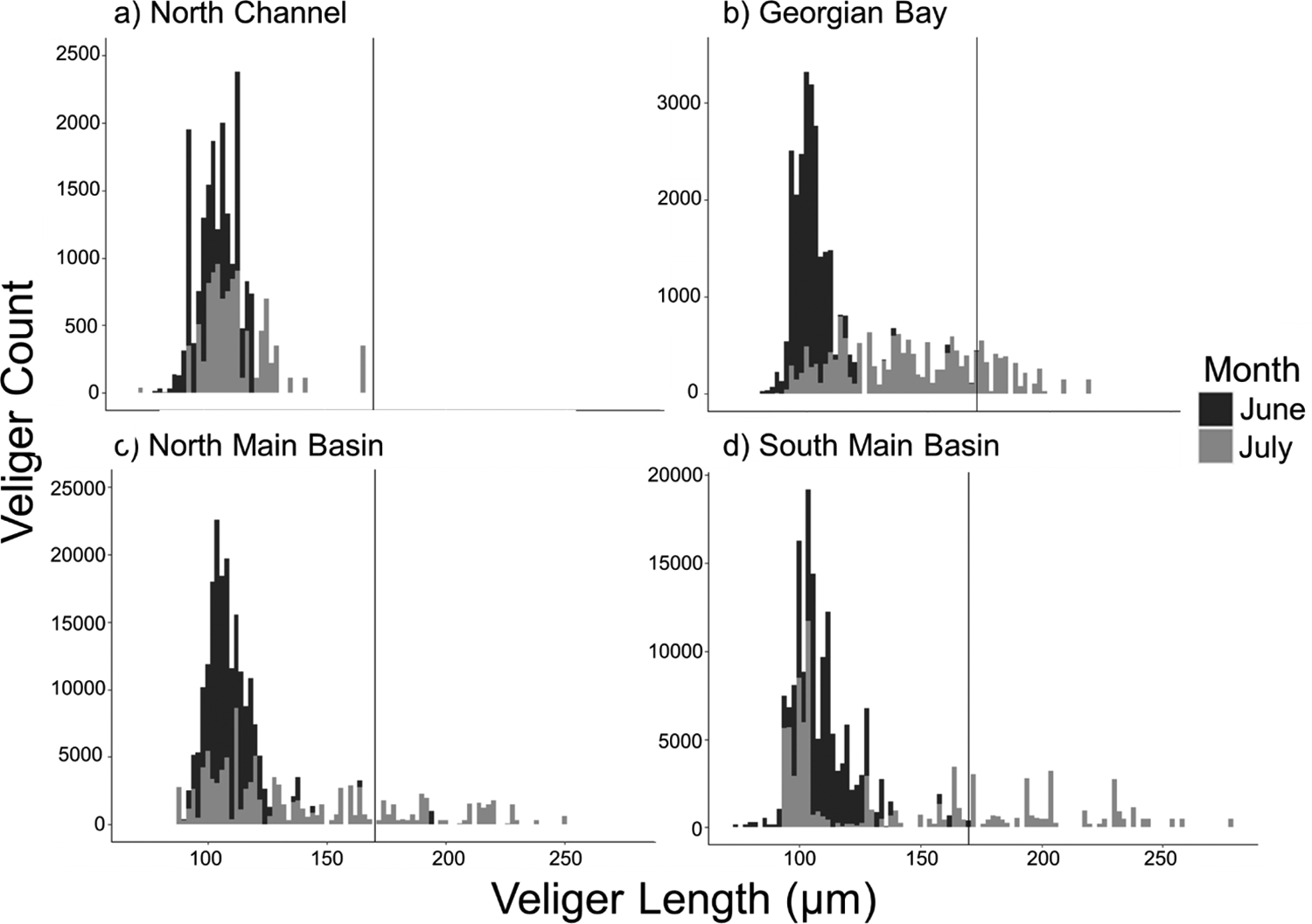
Histogram of pooled veliger length distributions (June – July) in each region. Bin width is 2 μm. A vertical line at 170 μm indicates “competent” veliger length.
The pooled length distributions of competent veligers in each basin were also non-normal. There was only one measurement (i.e., 171 μm in August) of a veliger large enough to be classified as “competent” in the North Channel, which limited our ability to compare this basin to the other basins. The median length of competent veligers was 180 μm in Georgian Bay, 195 μm in the North Main Basin, and 204 μm in the South Main Basin. Competent veligers comprised 8.28% of all veligers measured in this study. The percentages of competent veligers in each basin were relatively close to this proportion, except for the North Channel where it was 0.0005%. By contrast, the percentage of competent veligers measured in the other basins was closer to the lake-wide average: 9.02% in Georgian Bay, 8.55% in the North Main Basin, and 12.55% in the South Main Basin. Notably, these percentages increased dramatically from June to July within each basin: 0.03% to 23% in Georgian Bay, 0.73% to 21% in the North Main Basin, and 0.4% to 29.2 in the South Main Basin.
Index of Attrition
Our attrition rate estimate, calculated from the slope of the length distribution of veligers 104 μm and larger, was 0.032 for Lake Huron as a whole. However, attrition varied widely among basins (Fig. 4), with the North Channel estimated to be 0.071±0.0029, at least twice that of every other basin in the lake (i.e., 0.029±0.0026 in Georgian Bay, 0.025±0.0028 in the North Main Basin, 0.018±0.003 in the South Main Basin).
Fig. 4.

Attrition plots for veligers in each region of Lake Huron in June and July, excluding lengths less than 104 μm. Regression line plotted with shaded area representing the 95% confidence interval. The slope of those regression lines, reported in the equation, estimates the attrition rate. Negative count values indicate length bins with zero counts.
Explaining veliger density with environmental variables
Among the candidate GAMs (see Appendix A), the two most parsimonious ones (i.e., ΔAICc<2) included temperature, NOx, and chlorophyll a (Table 2). The top ranked model included temperature (F1 = 4.81, p = 0.035) and NOx (F3.1 = 3.04, p = 0.04). The second ranked model included temperature (F1 = 4.43, p = 0.04), NOx (F3.03 = 3.31, p = 0.03), and chlorophyll a (F1 = 1.82, p = 0.19). Veliger density was positively related to both temperature (Fig. 5a) and chlorophyll a (Fig. 5c), and the linear fit was better than a non-linear one. NOx was estimated to have non-linear, concave-up, unimodal curve relationship with veliger density, with peaks in veliger density occurring at both the minimum (193.7 μg/L) and maximum (363 μg/L) concentrations sampled (Fig. 5b). Calcium did not appear among the top ranked models.
Table 2.
Summary of model selection criteria (AICc = Akaike’s information criterion corrected for small samples sizes) for the two most parsimonious models (i.e., ΔAICc ≤2) among generalized additive models that sought to explain variation in veliger density using concentration of chlorophyll a, concentration of nitrates/nitrates (NOx), calcium, phosphorus and temperature (°C) as predictor variables (for a list of all candidate models see Appendix A). Fit statistics indicate that the variable was included in the model. An asterisk indicates that the variable was smoothed or non-linear. LogL indicates the log(likelihood) of the model. Weight is scaled from 0–1 and estimates the probability that a given model is actually the best among those considered.
| Version # | Chlorophyll α | NOx | Temperature | df | LogL | adj r2 | AICc | ΔAICc | Weight |
|---|---|---|---|---|---|---|---|---|---|
| 9 | F = 3.04, p = 0.04* | F = 4.81, p = 0.035 | 6.1 | −54.4 | 0.28 | 123.79 | 0 | 0.63 | |
| 7 | F = 1.82, p = 0.19 | F = 3.31, p = 0.03* | F = 4.43, p = 0.04 | 7 | −53.6 | 0.29 | 124.86 | 1.07 | 0.37 |
Fig. 5.

Relationship plots for the variables included among the top ranked models. Temperature (panel a) and NOx (panel b) are shown from the top-ranked model (see Table 2), whereas Chlorophyll a (panel c) is shown from the model with the 2nd lowest AICc value. For all panels, 95% confidence intervals are shown in the shaded area.
To explain the presence of competent veligers in July, the most parsimonious logistic model (ΔAICc<2; Appendix B) included only calcium as a predictor variable (F1 = 10.42, p = 0.001). The logistic model estimated the 50% probability of occurrence and identified a possible threshold value of calcium concentration required to promote maturation to competent veligers, as 21.84 mg/L (Fig. 6). Calcium concentrations in the North Channel in July averaged 20.99 mg/L, 22.58 mg/L in Georgian Bay and 24.12 mg/L in the North Main Basin. Unfortunately, we do not have data on the calcium concentration in the South Main Basin in July. In June and August, however, calcium concentrations in the South Main Basin averaged 26.59 mg/L and 24.94 mg/L, respectively, suggesting that calcium concentrations in July exceeded 21.84 mg/L.
Fig. 6.

Logistic regression plot showing the effect of calcium concentration (mg/L) on the presence probability of “competent” veligers in July 2017 within Lake Huron. The inflection point between the upper and lower levels is interpreted as the threshold value and is represented by the vertical line.
Discussion
To our knowledge, we are the first to report on the spring and summer Dreissena veliger densities and size structure across Lake Huron. Densities and biomasses of veligers were comparable between basins despite differences in density of benthic mussels across these regions (Karatayev et al., 2020). We found some variation between basins when looking at veliger length distributions and their respective attrition rates that may be due to differences in calcium concentration or other micro-nutrients. Using calcium concentrations and length data we also calculated a threshold calcium concentration of around 22 mg/L for veligers to survive and recruit to their juvenile and benthic adult life stages.
Given the low calcium levels, the high density and biomass of veligers in the North Channel indicates either a greater density of adult mussels in the North Channel than previously measured, or possibly an input of veligers from another source. Examining veliger densities by individual transects, it appears that the Spanish River transect is driving the high densities (e.g., exceeding 60,000 individuals/m3 in June and July) at the nearshore 18 m site. Comparatively, densities at Thessalon River (the only other transect in the North Channel) were much lower, never exceeding 3,000 individuals/m3 at the 18 m site. While the origin of these veligers is currently unknown, a possible explanation for the unexpectedly high density in North Channel is that there is a higher density of adult mussels than were reported in the 2017 CSMI benthos ponar survey (Karatayev et al., 2020) or in the benthos imaging survey (T. Angradi, personal communication), likely from regions with a hard substrate that were not accessed during sampling. One such local source could be regions within and around Manitoulin Island, which has a carbonate and sandstone bedrock compared to the granite and gneiss bedrock along the northern Ontario shore (Grannemann et al. 2000). Another possible explanation for unexpectedly high veliger densities in North Channel is movement of water containing veligers from another region. The main basin, however, is an unlikely source given that mean circulation patterns tend to be cyclonic and do not generally enter the North Channel but tend to remain in the main basin (Beletsky et al., 1999). Movement of water from Georgian Bay is more possible given that there is some outflow to the North Channel but the primary water exchange with Georgian Bay is with the main basin (Schertzer et al., 2008). Future research will be required to verify where the veligers in North Channel originate.
In addition to the variation among the North Channel transects, we also detected variation between transects within Georgian Bay. The Nottawasaga River 18 m site had a starkly greater density and biomass in June than in other months or stations in Georgian Bay: 71,107 individuals/m3 and a biomass of 10,548 μg/m3. Interestingly, the Nottawasaga watershed also has a carbonate and sandstone bedrock, whereas the French River watershed and Parry Sound region have granite and gneiss bedrock (Granneman et al. 2000). Unlike the North Channel, however, adult Dreissena are more abundant in Georgian Bay based on ponar sampling (Karatayev et al., 2020). This unusually high density and biomass at 18 m Nottawasaga could indicate that we sampled a pulse in Dreissena reproduction (Pothoven and Elgin, 2019).
The peak summer densities we observed in Lake Huron in 2017 are supported by some research, but inconsistencies with other studies suggest sporadic spawning conditions across the Great Lakes basin. The peaks in veliger density we observed in June and July are consistent with a study in the Saginaw River (tributary to Lake Huron) and in the Detroit River (flows from Lake St. Clair to Lake Erie) that collected mussels weekly or bi-weekly using an 80-μm mesh net (Ram et al., 2011). They identified a peak of veliger density in early June that was more than 5 times their previously sampled density in May; by August estimated densities were more similar to what was seen in May (Ram et al., 2011). Another study at three sites offshore of Muskegon, Michigan in Lake Michigan also found similar timing in peaks of veliger density, with different depth zones peaking in different times of the year based on bi-weekly sampling with a 64-μm mesh net (Pothoven and Elgin, 2019). Similar to our study, Pothoven and Elgin (2019) reported maximum densities occurring beginning in June/July, they also reported smaller local maxima in veliger density that occurred into October or even December, depending on the depths or years sampled. We did not sample into the fall, but our August sampling revealed a steeper decline in veliger densities in Lake Huron relative to early summer than what was measured in southern Lake Michigan. This may indicate that Dreissena in Lake Huron are more temporally synchronized in their spawning, or that the conditions in southern Lake Michigan create a longer window for spawning than they do in Lake Huron, or perhaps we would have seen similar local maxima had sampling continued into the fall. Another Lake Michigan study reported that spawning at 25-m sites occurred in mid-August and finished by November, while spawning at 45-m sites began in early June and finished by early August based on examination of the gonads of adult quagga mussels (Nalepa et al. 2010). If this pattern of nearshore Dreissena not spawning until later in the year also occurs in Lake Huron, it would suggest that the veligers we found in early summer were a result of spawning by Dreissena at the intermediate and offshore sites, and not the nearshore sites where the highest densities of veligers were found. This seems plausible because Nalepa et al. (2010) noted that spawning at one depth led to an increased density at the other depth, suggesting substantial horizontal mixing across depth regions.
The significantly greater density and biomass of veligers in the shallow (< 20 m) vertical depth layer than the deep (> 20 m) layer supports the EPA Great Lakes National Program Office standard operating practice of sampling only the top 20 m of the water column for small-mesh zooplankton surveys (a decision driven more by net clogging than presumed veliger spatial patterns). These results also align with a previous study by Bowen et al. (2018) that showed mean values of veligers in the meta- and hypolimnion were two to four times lower than in the epilimnion. Even though sampling in the shallow layer may accurately represent veliger density, sampling deeper water layers would be beneficial for more comprehensive studies of veliger dynamics and improved understanding of veliger maturation and settlement. For example, it is possible that later in the season length distributions may differ at different vertical layers as more mature individuals move towards the benthos to settle.
The concentration of competent veligers is strongly correlated (r = 0.93–0.98) with the daily settlement rate of zebra mussels (Martel et al., 1994). Because competent veligers were only sampled in North Channel at one site in one month, it is likely that daily settlement rates there are very low. While the South Main Basin had the largest proportion of veligers above the competent threshold size, the North Main Basin had the greatest mean density of competent veligers, suggesting that the daily settlement rate of veligers in the North Main Basin may be greater than in the other basins of the lake. However, it is important to note that the period of post-settlement may be a time of high mortality (Martel et al., 1994) and that settlement rates may not reflect future densities of adult mussels. Additionally, because we found that the greatest densities of competent veligers occurred almost entirely in July with very few in August, we can assume that the period of greatest daily settlement during our sampling period was also during July.
We hypothesize that our observations of lower median veliger length in the North Channel, only sampling one competent-sized veliger, and the highest rate of attrition were the result of insufficient calcium concentrations to sustain further development of veligers into juvenile mussels. Indeed, we found that the North Channel had lower average levels of calcium (19.1 mg/L) than the other basins (22.5 – 26 mg/L), perhaps reflective of the differences in bedrock composition (Granneman et al. 2000). In a meta-analysis of more than 3,000 stream and rivers sites across the U.S., Whittier et al. (2008) classified calcium concentrations less than 20 mg/L to be “low risk” for invasion by Dreissena (Whittier et al., 2008). Calcium concentrations ranging from 20–28 mg/L were considered “moderate” risk which encompasses the other Lake Huron basins that we sampled. We only found one experiment that evaluated survival of different life stages of quagga mussels as a function of calcium limitation, and it was supportive of our hypothesis. Veliger survival for the first 30 days gradually increased with increasing calcium concentrations, from 30% survival at 12 mg/L, 40% at 21 mg/L, to 95% at 72 mg/L (Davis et al., 2015). Interestingly, these results did not necessarily conform to the threshold survival response to calcium concentrations at around 22 mg/L that our logistic model predicted. Furthermore, Davis et al. (2015) reported adult survival to exceed 75% at calcium concentrations of 12 mg/L and higher. Hence these experimental results suggest that adults in North Channel have enough calcium to survive and our veliger sampling suggests that those few surviving there are producing veligers. This could explain why calcium concentrations were not a predictor of veliger density in our GAM results. Given that densities and biomass of veligers in the North Channel were comparable with every other basin in each month despite a lower concentration of calcium, we propose that calcium in the North Channel is not preventing survival of adults or their reproductive success or production of veligers, but maturation and survival from the larval to juvenile settlement stage. We encourage additional research to test our hypothesis, and to explore other micronutrients that could be affecting survival of different life stages of Dreissena in North Channel.
Variation in veliger density was explained by several environmental variables other than calcium. Temperature and NOx were the most frequently selected predictor variables among the top ranked GAMs. Temperature is vital in determining the growth rate of veligers, the filtration efficiency of veligers and adults, and the length of the reproductive window (Bowen et al., 2018; Nalepa et al., 2007). Our finding that veliger density increases with higher concentrations of chlorophyll (a proxy for their phytoplankton prey) is consistent with our original hypothesis. The role of NOx and its influence in determining veliger density is less clear. Previous studies have found that increasing concentrations of NOx result in lower densities of Dreissena (Ramcharan et al., 1992) and our finding of a non-linear relationship, negative until roughly 275 μg/L then positive, was unexpected and more investigation is required to determine whether the mechanism is causative or not.
A number of systemic changes are underway in the Great Lakes that may impact the attrition rates and survivorship of veligers in the future. One of these changes is a general decrease in phytoplankton abundance (commonly attributed to benthic Dreissena sequestering phosphorus and other nutrients) as well as changes in the phytoplankton community composition (Reavie et al., 2014). Veligers have been found to feed on bacteria, blue-green algae, and small green algae from 1–4 μm in diameter (Sprung, 1992). In neighboring Lake Michigan, Carrick et. al (2015) investigated the relative abundance of several size classes of phytoplankton and found that while total abundance of phytoplankton in the lake has decreased, the relative abundance of phytoplankton in the picoplankton class (particles <2 μm) increased twofold. If a similar increase in picoplankton has occurred in Lake Huron, the positive relationship we observed between veliger density and chlorophyll a may have been indicative of more available prey for veligers. An additional factor that could enhance veliger density is the long-term warming of the Great Lakes (Mason et al., 2016; Zhong et al., 2016). Given that most veligers occur in the epilimnetic waters which may also be the most sensitive to increasing air temperatures, it is likely that the growth rate, filtration efficiency, and length of the reproductive window will all increase for quagga mussels in Lake Huron (Bowen et al., 2018; Karatayev et al., 2015).
In this study, we provided new knowledge on an understudied life stage of Dreissena, its larval and planktonic veligers. We increased understanding of spatial and temporal patterns in Dreissena veligers throughout Lake Huron, highlighted mismatches with spatial patterns for settled mussels, and sought to explain why veligers might not survive to competence in the North Channel. We put forward new information regarding the environmental tolerances of Dreissena veligers in Lake Huron and illustrated how calcium concentrations below 20 mg/L do not limit production and survival of young veligers, but instead may limit survival of larger and older veligers, thus preventing settlement. Further understanding of the environmental tolerances of quagga mussels and life-stage based population dynamics of Dreissena could provide more accurate assessments of the health of invaded bodies of water, better judgements of invasion threat in as-yet untouched systems and could inform the development of new methods of control.
Supplementary Material
Acknowledgements
We acknowledge the efforts of multiple individuals that assisted in different aspects of this study. We appreciate the vessel crews of multiple federal research vessels: R/V Arcticus, R/V Sturgeon, R/V Lake Guardian, and R/V Lake Explorer II. Many scientists contributed to the field sampling efforts on these vessels, especially Amelia Runco, Matt Welc, and Dave Warner from USGS, Paris Collingsworth and Joel Hoffman from EPA. Ann Cotter deserves additional credit not only for field work but also for organizing water quality sampling on USGS vessels and for processing all of the water quality samples in Duluth. We thank Yu-Chun Kao and Lindsie Egedy for statistical advice. We appreciate the helpful insights from Todd Howell and Erin Dunlop on interpreting calcium concentrations across Lake Huron. This manuscript was improved from helpful comments from Clay Kirkendall and Andrea Negele. Funding was provided from the EPA Great Lakes Restoration Initiative. Preliminary analyses of these data by Darren Kirkendall was supported by the ESA/USGS Cooperative Summer Field Training Program in 2019. Any use of trade, firm, or product names is for descriptive purposes only and does not imply endorsement by the US Government.
Appendices
Appendix A. Summary of model selection criteria in order of AICc score (AICc = Akaike’s information criterion corrected for small samples sizes) among generalized additive models that sought to explain variation in veliger density using concentration of calcium, chlorophyll a, nitrates/nitrates (NOx), temperature, and phosphorus as predictor variables. LogL indicates the log(likelihood) of the model. Fit statistics indicate that the variable was included in the model. An asterisk indicates that the variable was smoothed or non-linear.
| Version # | Calcium | Chlorophyll α | NOx | Temperature | Phosphorus | df | LogL | adj r2 |
|---|---|---|---|---|---|---|---|---|
| 9 | F = 3.04, p = 0.04* | F = 4.81, p = 0.035 | 6.1 | −54.44 | 0.28 | |||
| 7 | F = 1.82, p = 0.19 | F = 3.31, p = 0.03* | F = 4.43, p = 0.04 | 7 | −53.58 | 0.29 | ||
| 12 | F = 2.79, p = 0.04* | 4.95 | −57.34 | 0.19 | ||||
| 2 | F = 4.26, p = 0.046 | F = 8.03, p = 0.008 | 4 | −58.65 | 0.16 | |||
| 6 | F = 2.93, p = 0.04* | F = 4.73, p = 0.04 | F = 0.08, p = 0.77 | 7.1 | −54.37 | 0.26 | ||
| 11 | F = 2.07, p = 0.16 | F = 2.91, p = 0.04* | 5.93 | −56.28 | 0.21 | |||
| 5 | F = 1.7, p = 0.2 | F = 3.11, p = 0.03* | F = 4.11, p = 0.051 | F = 0.003, p = 0.96 | 8 | −53.59 | 0.27 | |
| 19 | F = 4.42, p = 0.04 | 3 | −60.83 | 0.08 | ||||
| 1 | F = 4.06, p = 0.052 | F = 6.31, p = 0.02 | F = 0.05, p = 0.83 | 5 | −58.63 | 0.13 | ||
| 10 | F = 2.34, p = 0.08* | F = 0.05, p = 0.83 | 5.91 | −57.36 | 0.17 | |||
| 8 | F = 2.16, p = 0.15 | F = 2.42, p = 0.07* | F = 0.19, p = 0.67 | 6.87 | −56.27 | 0.19 | ||
| 15 | F = 0.68, p = 0.42 | F = 3.56, p = 0.07 | 4 | −60.47 | 0.07 | |||
| 14 | F = 3.22, p = 0.08 | F = 0.12, p = 0.73 | 4 | −60.77 | 0.06 | |||
| 18 | F = 1.4, p 0.24 | 3 | −62.31 | 0.01 | ||||
| 17 | F = 1.15, p = 0.29 | 3 | −62.44 | 0.004 | ||||
| 4 | F = 0.87, p = 0.36 | 3 | −62.58 | 0.003 | ||||
| 16 | F = 1.63, p = 0.21 | F = 1.38, p = 0.25 | 4 | −61.57 | 0.02 | |||
| 13 | F = 0.78, p = 0.38 | F = 2.29, p = 0.14 | F = 0.24, p = 0.63 | 5 | −60.34 | 0.05 | ||
| 3 | F = 1.08, p = 0.31 | F = 1.36, p = 0.25 | 4 | −61.86 | 0.006 |
Appendix B. Summary of model selection criteria in order of AICc score (AICc = Akaike’s information criterion corrected for small samples sizes) among logistic models that sought to explain the presence probability of competent veligers using concentration of calcium, chlorophyll a, nitrates/nitrates (NOx), temperature, and phosphorus as predictor variables. LogL indicates the log(likelihood) of the model. Fit statistics indicate that the variable was included in the model.
| Version # | Calcium | Chlorophyll α | NOx | Temperature | Phosphorus | df | LogL | AICc | ΔAICc |
|---|---|---|---|---|---|---|---|---|---|
| 4 | F = 10.42, p = 0.001 | 2 | −4.88 | 14.77 | 0 | ||||
| 2 | F = 10.42, p = 0.001 | F = 0.46, p = 0.5 | 3 | −4.65 | 17.49 | 2.72 | |||
| 3 | F = 10.42, p = 0.001 | F = 0.35, p = 0.6 | 3 | −4.71 | 17.59 | 2.82 | |||
| 1 | F = 10.42, p = 0.001 | F = 0.45, p = 0.5 | F = 0.56, p = 0.45 | 4 | −4.37 | 20.75 | 5.98 | ||
| 17 | F = 4.3, p = 0.03 | 2 | −7.95 | 20.89 | 6.12 | ||||
| 11 | F = 4.55, p = 0.03 | F = 2.25, p = 0.13 | 3 | −6.7 | 21.58 | 6.81 | |||
| 12 | F = 2.25, p = 0.13 | 2 | −8.97 | 22.94 | 8.17 | ||||
| 16 | F = 3.82, p = 0.05 | F = 0.61, p = 0.43 | 3 | −7.88 | 23.94 | 9.17 | |||
| 14 | F = 4.3, p = 0.04 | F = 0.004, p = 0.95 | 3 | −7.94 | 24.07 | 9.3 | |||
| 9 | F = 2.25, p = 0.13 | F = 1.64, p = 0.2 | 3 | −8.15 | 24.49 | 9.72 | |||
| 18 | F = 0.61, p = 0.43 | 2 | −9.79 | 24.58 | 9.81 | ||||
| 19 | F = 0.09, p = 0.76 | 2 | −10.05 | 25.1 | 10.33 | ||||
| 7 | F = 3.04, p = 0.08 | F = 2.25, p = 0.13 | F = 1.64, p = 0.2 | 4 | −6.63 | 25.27 | 10.5 | ||
| 8 | F = 4.55, p = 0.03 | F = 2.25, p = 0.13 | F = 0.009, p = 0.92 | 4 | −6.69 | 25.39 | 10.62 | ||
| 10 | F = 2.25, p = 0.13 | F = 0.003, p = 0.96 | 3 | −8.97 | 26.12 | 11.35 | |||
| 15 | F = 0.61, p = 0.43 | F = 0.07, p = 0.8 | 3 | −9.75 | 27.69 | 12.92 | |||
| 13 | F = 3.82, p = 0.05 | F = 0.61, p = 0.43 | F = 0.0004, p = 0.98 | 4 | −7.88 | 27.76 | 12.99 | ||
| 6 | F = 2.25, p = 0.13 | F = 1.64, p = 0.2 | F = 0.03, p = 0.9 | 4 | −8.14 | 28.28 | 13.51 | ||
| 5 | F = 3.04, p = 0.08 | F = 2.25, p = 0.13 | F = 1.64, p = 0.2 | F = 0.03, p = 0.9 | 5 | −6.62 | 29.9 | 15.13 |
References
- Ackerman JD, Sim B, Nichols SJ, Claudi R, 1994. A review of the early life history of zebra mussels (Dreissena polymorpha): comparisons with marine bivalves. Can. J. of Zool 72, 1169–1179. 10.1139/z94-157 [DOI] [Google Scholar]
- American Public Health Association, American Water Works Association, Water Pollution Control Federation and Water Environment Federation, 1998. Standard methods for the examination of water and wastewater. 20th ed. American Public Health Association. [Google Scholar]
- Barbiero RP, Balcer M, Rockwell DC, Tuckman ML, 2009. Recent shifts in the crustacean zooplankton community of Lake Huron. Can. J. Fish. Aquat. Sci 66, 816–828. 10.1139/F09-036 [DOI] [Google Scholar]
- Barbiero RP, Lesht BM, Warren GJ, Rudstam LG, Watkins JM, Reavie ED, Kovalenko KE, Karatayev AY, 2018. A comparative examination of recent changes in nutrients and lower food web structure in Lake Michigan and Lake Huron. J. Gt. Lakes Res 44, 573–589. 10.1016/j.jglr.2018.05.012 [DOI] [PMC free article] [PubMed] [Google Scholar]
- Barton Kamil., 2019. MuMIn: Multi-Model Inference. R package version 1.43.6. https://CRAN.R-project.org/package=MuMIn. [Google Scholar]
- Beletsky D, Saylor JH, Schwab DJ, 1999. Mean Circulation in the Great Lakes. J. Gt. Lakes Res 25, 78–93. 10.1016/S0380-1330(99)70718-5 [DOI] [Google Scholar]
- Benson AJ, Richerson MM, Maynard E, Larson J, Fusaro A, Bogdanoff AK, Neilson ME, and Elgin Ashley, 2020a, Dreissena rostriformis bugensis (Andrusov, 1897): U.S. Geological Survey, Nonindigenous Aquatic Species Database, Gainesville, FL, and NOAA Great Lakes Aquatic Nonindigenous Species Information System, Ann Arbor, MI, https://nas.er.usgs.gov/queries/greatLakes/FactSheet.aspx?SpeciesID=95&Potential=N&Type=0&HUCNumber=DGreatLakes, Revision Date: 9/13/2019, Access Date: 6/4/2020 [Google Scholar]
- Benson AJ, Raikow D, Larson J, Fusaro A, Bogdanoff AK, and Elgin A, 2020b, Dreissena polymorpha (Pallas, 1771): U.S. Geological Survey, Nonindigenous Aquatic Species Database, Gainesville, FL, and NOAA Great Lakes Aquatic Nonindigenous Species Information System, Ann Arbor, MI, https://nas.er.usgs.gov/queries/greatLakes/FactSheet.aspx?SpeciesID=5&Potential=N&Type=0&HUCNumber=DGreatLakes, Revision Date: 6/2/2020, Access Date: 6/4/2020
- Bowen KL, Conway AJ, Currie WJS, 2018. Could dreissenid veligers be the lost biomass of invaded lakes? Freshw. Sci 37, 315–329. 10.1086/697896 [DOI] [Google Scholar]
- Burnham KP, Anderson DR, 2002. Model selection and multimodel inference. Springer-Verlag, New York. [Google Scholar]
- Carlton JT, 2008. The Zebra Mussel Dreissena polymorpha Found in North America in 1986 and 1987. J. Gt. Lakes Res 34, 770–773. 10.1016/S0380-1330(08)71617-4 [DOI] [Google Scholar]
- Carrick HJ, Butts E, Daniels D, Fehringer M, Frazier C, Fahnenstiel GL, Pothoven S, Vanderploeg HA, 2015. Variation in the abundance of pico, nano, and microplankton in Lake Michigan: Historic and basin-wide comparisons. J. Gt. Lakes Res 41, 66–74. 10.1016/j.jglr.2015.09.009 [DOI] [Google Scholar]
- Chapman DG, Robson DS, 1960. The Analysis of a Catch Curve. Biometrics 16, 354. 10.2307/2527687 [DOI] [Google Scholar]
- Davis CJ, Ruhmann EK, Acharya K, Chandra S, Jerde CL, 2015. Successful survival, growth, and reproductive potential of quagga mussels in low calcium lake water: is there uncertainty of establishment risk? PeerJ; San Diego. 10.7717/peerj.1276 [DOI] [PMC free article] [PubMed] [Google Scholar]
- Evans MA, Fahnenstiel G, and Scavia D. 2011. Incidental oligotrophication of North American Great Lakes. Environ. Sci. Technol 45, 3297–3303. [DOI] [PubMed] [Google Scholar]
- Garton D, McMahon R, Stoeckmann N, 2014. Limiting Environmental Factors and Competetive Interactions between Zebra and Quagga Mussels in North America, in: Nalepa TF, Schloesser DW, Quagga and Zebra Mussels: Biology, Impacts, and Control. CRC Press, Taylor & Francis Group, Boca Raton, pp. 383–398. [Google Scholar]
- Grannemann NG, Hunt RJ, Nicholas JR, Reilly TE, Winter TC, 2000. The Importance of Ground Water in the Great Lakes Region (Water-Resources Investigations Report No. 00-4008). U.S. Geological Survey. [Google Scholar]
- Hebert PDN, Wilson CC, Murdoch MH, Lazar R, 1991. Demography and ecological impacts of the invading mollusc Dreissena polymorpha. Can. J. Zool 69, 405–409. 10.1139/z91-063 [DOI] [Google Scholar]
- Hecky RE, Smith RE, Barton DR, Guildford SJ, Taylor WD, Charlton MN, Howell T, 2004. The nearshore phosphorus shunt: a consequence of ecosystem engineering by dreissenids in the Laurentian Great Lakes. Can. J. Fish. Aquat. Sci 61, 1285–1293. 10.1139/f04-065 [DOI] [Google Scholar]
- Holland RE, 1993. Changes in Planktonic Diatoms and Water Transparency in Hatchery Bay, Bass Island Area, Western Lake Erie Since the Establishment of the Zebra Mussel. J. Gt. Lakes Res 19, 617–624. 10.1016/S0380-1330(93)71245-9 [DOI] [Google Scholar]
- Holland RE, Johengen TH, Beeton AM, 1995. Trends in nutrient concentrations in Hatchery Bay, western Lake Erie, before and after Dreissena polymorpha. Can. J. Fish. Aquat. Sci 52, 1202–1209. 10.1139/f95-117 [DOI] [Google Scholar]
- Karatayev AY, Burlakova LE, Padilla DK, 2002. Impacts of Zebra Mussels on Aquatic Communities and their Role as Ecosystem Engineers, in: Leppäkoski E, Gollasch S, Olenin S (Eds.), Invasive Aquatic Species of Europe. Distribution, Impacts and Management. Springer; Netherlands, Dordrecht, pp. 433–446. 10.1007/978-94-015-9956-6_43 [DOI] [Google Scholar]
- Karatayev AY, Burlakova LE, Padilla DK, 2015. Zebra versus quagga mussels: a review of their spread, population dynamics, and ecosystem impacts. Hydrobiologia; Dordrecht 746, 97–112. http://dx.doi.org.mutex.gmu.edu/10.1007/s10750-014-1901-x [Google Scholar]
- Karatayev AY, Burlakova LE, Mehler K, Daniel SE, Elgin AK, Nalepa TF, 2020. Lake Huron Benthos Survey, Cooperative Science and Monitoring Initiative 2017, Technical Report 48.
- Klerks PL, Fraleigh PC, Lawniczak JE, 1996. Effects of zebra mussels (Dreissena polymorpha) on seston levels and sediment deposition in western Lake Erie 53, 11. [Google Scholar]
- MacIsaac HJ, Sprules WG, Leach JH, 1991. Ingestion of Small-Bodied Zooplankton by Zebra Mussels (Dreissena polymorpha): Can Cannibalism on Larvae Influence Population Dynamics? Can. J. Fish. Aquat. Sci 48, 2051–2060. 10.1139/f91-244 [DOI] [Google Scholar]
- MacIsaac HJ, Sprules WG, Johannsson OE, Leach JH, 1992. Filtering Impacts of Larval f30–39. [DOI] [PubMed]
- Martel A, Mathieu AF, Findlay CS, Nepszy SJ, Leach JH, 1994. Daily Settlement Rates of the Zebra Mussel, Dreissena polymorpha, on an Artificial Substrate Correlate with Veliger Abundance. Can. J. Fish. Aquat. Sci 51, 856–861. 10.1139/f94-084 [DOI] [Google Scholar]
- Mason LA, Riseng CM, Gronewold AD, Rutherford ES, Wang J, Clites A, Smith SDP, McIntyre PB, 2016. Fine-scale spatial variation in ice cover and surface temperature trends across the surface of the Laurentian Great Lakes. Climatic Change 138, 71–83. 10.1007/s10584-016-1721-2 [DOI] [Google Scholar]
- Mills EL, Dermott RM, Roseman EF, Dustin D, Mellina E, Conn DB, Spidle AP, 1993. Colonization, Ecology, and Population Structure of the “Quagga” Mussel (Bivalvia: Dreissenidae) in the Lower Great Lakes. Can. J. Fish. Aquat. Sci 50, 2305–2314. 10.1139/f93-255 [DOI] [Google Scholar]
- Nalepa TF, Fanslow DL, Pothoven SA, Foley AJ, Lang GA, 2007. Long-term Trends in Benthic Macroinvertebrate Populations in Lake Huron over the Past Four Decades. J. Gt. Lakes Res 33, 421–436. 10.3394/0380-1330(2007)33[421:LTIBMP]2.0.CO;2 [DOI] [Google Scholar]
- Nalepa TF, Fanslow DL, Pothoven SA, 2010. Recent changes in density, biomass, recruitment, size structure, and nutritional state of Dreissena populations in southern Lake Michigan. J. Gt. Lakes Res 36, 5–19. 10.1016/j.jglr.2010.03.013 [DOI] [Google Scholar]
- Nowicki C, Bunnell DB, Armenio PM, Warner DM, Vanderploeg HA, Cavaletto J, Mayer C, Adams JV, 2017. Biotic and Abiotic Factors Influencing Zooplankton Vertical Distribution in Lake Huron. J. Gt. Lakes Res 43, 1044–1054. [Google Scholar]
- Pothoven SA, Elgin AK, 2019. Dreissenid veliger dynamics along a nearshore to offshore transect in Lake Michigan. J. Gt. Lakes Res 45, 300–306. 10.1016/j.jglr.2019.01.001 [DOI] [Google Scholar]
- R Core Team (2019). R: A language and environment for statistical computing. R Foundation for Statistical Computing, Vienna, Austria. https://www.R-project.org/. [Google Scholar]
- Ram J, Karim A, Acharya P, Jagtap P, Purohit S, Kashian D, 2011. Reproduction and Genetic Detection of Veligers in Changing Dreissena Populations in the Great Lakes. Ecosphere 2, 1–16. [Google Scholar]
- Ramcharan CW, Padilla DK, Dodson SI, 1992. Models to Predict Potential Occurrence and Density of the Zebra Mussel, Dreissena polymorpha. Can. J. Fish. Aquat. Sci 49, 2611–2620. 10.1139/f92-289 [DOI] [Google Scholar]
- Reavie ED, Barbiero RP, Allinger LE, Warren GJ, 2014. Phytoplankton trends in the Great Lakes, 2001–2011. J. Gt. Lakes Res 40, 618–639. 10.1016/j.jglr.2014.04.013 [DOI] [Google Scholar]
- Schertzer WM, Assel RA, Beletsky D, Croley TE, Lofgren BM, Saylor JH, Schwab DJ, 2008. Lake Huron climatology, inter-lake exchange and mean circulation. Aquat. Ecosyst. Health Manag 11, 144–152. 10.1080/14634980802098705 [DOI] [Google Scholar]
- SOP LG403. 2016. Standard Operating Procedure for Zooplankton Analysis. Revision 07, July 2016. Great Lakes National Program Office, U.S. Environmental Protection Agency., Chicago, IL. [Google Scholar]
- Sprung M, 1992. The Other Life: An Account of Present Knowledge of the Larval Phase of Dreissena polymorpha, in: Zebra Mussels Biology, Impacts, and Control. pp. 39–53. [Google Scholar]
- Vanderploeg HA, Liebig JR, Carmichael WW, Agy MA, Johengen TH, Fahnenstiel GL, Nalepa TF, 2001. Zebra mussel (Dreissena polymorpha) selective filtration promoted toxic Microcystis blooms in Saginaw Bay (Lake Huron) and Lake Erie. Can. J. Fish. Aquat. Sci 58, 1208–1221. 10.1139/f01-066 [DOI] [Google Scholar]
- Vanderploeg HA, Nalepa TF, Jude DJ, Mills EL, Holeck KT, Liebig JR, Grigorovich IA, Ojaveer H, 2002. Dispersal and emerging ecological impacts of Ponto-Caspian species in the Laurentian Great Lakes. Can. J. Fish. Aquat. Sci 59, 1209–1228. 10.1139/f02-087 [DOI] [Google Scholar]
- Vanderploeg HA, Wilson A, Johengen TH, Bressie J, Sarnelle O, Liebig JR, Robinson S, Horst Geoffrey, 2014. Role of Selective Grazing by Dreissenid Mussels in Promoting Toxic Microcystis Blooms and Other Changes in Phytoplankton Composition in the Great Lakes, in: Quagga and Zebra Mussels: Biology, Impacts, and Control. [Google Scholar]
- Welschmeyer NA, 1994. Fluorometric analysis of chlorophyll a in the presence of chlorophyll b and pheopigments. Limnol. Oceanogr, 39(8), pp.1985–1992. [Google Scholar]
- Whitten AL, Marin Jarrin JR, McNaught AS, 2018. A mesocosm investigation of the effects of quagga mussels (Dreissena rostriformis bugensis) on Lake Michigan zooplankton assemblages. J. Gt. Lakes Res 44, 105–113. 10.1016/j.jglr.2017.11.005 [DOI] [Google Scholar]
- Whittier TR, Ringold PL, Herlihy AT, Pierson SM, 2008. A calcium-based invasion risk assessment for zebra and quagga mussels (Dreissena spp). Frontiers in Ecology and the Environment 6, 180–184. 10.1890/070073 [DOI] [Google Scholar]
- Wickham H, 2016. ggplot2: Elegant Graphics for Data Analysis. Springer-Verlag, New York. [Google Scholar]
- Wood SN, 2006. Generalized additive models: an introduction with R. CRC Press, Boca Raton, Florida. [Google Scholar]
- Wood SN, 2008. Fast stable direct fitting and smoothness selection for generalized additive models. J. R. Statistical Society Series B: Statistical Methodology 70, 495–518. [Google Scholar]
- Zhong Y, Notaro M, Vavrus SJ, Foster MJ, 2016. Recent accelerated warming of the Laurentian Great Lakes: Physical drivers. Limnol. Oceanogr 61, 1762–1786. 10.1002/lno.10331 [DOI] [Google Scholar]
Associated Data
This section collects any data citations, data availability statements, or supplementary materials included in this article.