Evaluation of the risks for animal health related to the presence of hydroxymethylfurfural (HMF) in feed for honey bees

Abstract

The European Commission has asked the EFSA to evaluate the risk for animal health related to the presence of hydroxymethylfurfural (HMF) in honey bee feed. HMF is a degradation product of particular sugars and can be present in bee feed. HMF is of low acute toxicity in bees but causes increased mortality upon chronic exposure. A benchmark dose lower limit 10% (BMDL₁₀) of 1.16 μg HMF per bee per day has been calculated from mortalities observed in a 20‐day study and established as a Reference Point covering also mortality in larvae, drones and queens for which no or insufficient toxicity data were available. Winter bees have a much longer lifespan than summer bees and HMF shows clear time reinforced toxicity (TRT) characteristics. Therefore, additional Reference Point intervals of 0.21–3.1, 0.091–1.1 and 0.019–0.35 µg HMF/bee per day were calculated based on extrapolation to exposure durations of 50, 90 and 180 days, respectively. A total of 219 analytical data of HMF concentrations in bee feed from EU Member States and 88 from Industry were available. Exposure estimates of worker bees and larvae ranged between 0.1 and 0.48, and between 0.1 and 0.51 μg HMF/per day, respectively. They were well below the BMDL₁₀ of 1.16 μg HMF/bee per day, and thus, no concern was identified. However, when accounting for TRT, the probability that exposures were below established reference point intervals was assessed to be extremely unlikely to almost certain depending on exposure duration. A concern for bee health was identified when bees are exposed to HMF contaminated bee feed for several months.

Summary

Following a request from the European Commission, the European Food Safety Authority (EFSA) Panel on Contaminants in the Food Chain (CONTAM Panel) evaluated the risks for animal health related to the presence of hydroxymethylfurfural (HMF) in feed for honey bees. Relevant general EFSA guidance and specific guidance for honey bees were applied for the risk assessment conducted in this opinion. The draft Opinion underwent a public consultation from 3 December 2021 to 10 February 2022. The comments received and how they were taken into account when finalising the scientific Opinion are available in Annex A to this scientific Opinion.

5‐Hydroxymethylfurfural (HMF) is a degradation product of hexoses and is present in honey and various bee feeds. Commercially available bee feeds contain either sucrose or mixtures of glucose and fructose and may contain varying levels of HMF depending on the conditions of production and use. The most important parameters for HMF formation in bee feeds are the type of sugar used, pH, temperature, water activity and concentration of divalent cations of the media. HMF is determined by spectrometric and chromatographic methods.

While the toxicokinetics of HMF are well investigated in mammals, no information on the toxicokinetics of HMF in honey bees could be identified. Several experimental studies have been carried out in which the effect of oral uptake of HMF in bees on mortality/survival was investigated and the concentrations of HMF causing mortality in experimental studies varied between 150 and 750 mg/kg bee feed. It was observed that HMF induced mortality in bees strongly aggravates with exposure time. However, field studies with bees ingesting HMF containing bee feed suggest that feeding with concentrations between 40 and 150 mg HMF/kg bee feed is not detrimental to bee colonies.

The mode of action by which HMF induces bee mortality has not been elucidated but it has been shown that HMF causes histopathological effects in the midgut of bees which were paralleled by increased mortality.

Based on the absence of acute toxicity even at high doses, HMF is considered to be of low acute toxicity. Increased mortality (decreased survival) rate has been identified as the critical chronic effect of HMF in bees. Three experimental studies have been identified as suitable for assessing the chronic concentration/dose response in worker bees. A benchmark response (BMR) of 10% was identified as appropriate for the critical endpoint. Benchmark doses lower limit 10% (BMDL₁₀) of 32.7 μg/bee per day, 1.16 μg/bee per day and of 18.0 μg/bee per day were calculated from each of the three studies. A reference point (RP) of 1.16 μg HMF/bee per day was derived based on the lowest BMDL₁₀ seen in the three suitable studies. This was considered as the primary BMDL₁₀ for risk characterisation, even though it was substantially lower than the BMDL₁₀ obtained from the other two studies suitable for risk assessment. The RP of 1.16 μg HMF/bee per day also covers HMF‐induced mortality in larvae, drones and queens for which no or only insufficient data are available.

Since analyses indicated that HMF has clear time reinforced toxicity (TRT) characteristics, additional RPs were established. Based on extrapolation factors calculated from results associated with the TRT assessment adjusted RP intervals, reflecting uncertainty across the two studies used for the TRT assessment, of 0.21–3.1, 0.091–1.1, 0.019–0.35 µg/bee per day were derived for exposure durations of 50, 90 and 180 days, respectively.

A total of 219 analytical samples of bee feed from three different European Member States and 88 analytical results with bee feed from a European company were available. Data on consumption of bee feed were not available. Therefore, the default consumption value of 8.8 mg sugar/bee for thermoregulation of worker bees from the respective EFSA opinion on risk assessment for pesticides in bees was used for the exposure assessment. For larvae, a consumption value of 9.3 mg sugar per day reported in the public literature was used for exposure assessments. To calculate the feed intakes for the exposure assessment, a 72% dry matter content was used.

Exposure scenarios for worker bees have been calculated with the HMF levels reported in the data sets from Member States (data set A) and Industry (data set B) assuming exclusive consumption of bee feed and using consumption values as described above. For worker bees, using average HMF concentrations, the highest exposure estimates at lower bound/upper bound (LB/UB) were 0.47/0.48 μg/bee per day for the subset of complementary feed (n = 95) from European Member States (data set A). When combining the data on complementary feed, complete feed and sugar syrup (n = 216), an exposure of 0.32/0.33 μg HMF/bee per day was obtained. Using the data from Industry (data set B), exposures, depending on storage time of bee feed, varied between 0.29 and 0.34 μg/bee per day. For larvae, exposure estimates at LB/UB were 0.50/0.51 μg/larva per day for complementary feed. With the complete data set from European Member States, an exposure of 0.34 μg/larva per day was derived. Using Industry data, exposures, depending on storage time of bee feed, ranged between 0.31 and 0.44 μg HMF/larva per day.

Considering a brand loyalty exposure scenario using the P95 concentrations from data set A driven by a few exceptionally high occurrence values which are about an order of magnitude higher than those usually observed in bee feed and which are likely the result of inappropriate production/storage conditions of the feed, P95 exposures of worker bees/larvae of up to 4.40 and 4.65 μg HMF per day could result.

The range of mean exposure scenarios for worker bees across data sets A and B in was 0.1–0.48 μg/bee per day, are all below the RP of 1.16 μg HMF/bee per day. Based on the uncertainty analysis, it is regarded almost impossible (probability < 1%) that the reference point for 20 days of exposure is exceeded. Considering the mortality rates that would trigger a concern for bee health as laid down in the protection goals defined for honey bees (i.e. a 10% reduction in colony size), the CONTAM Panel did not identify a concern for the health of worker bees due to exposure to HMF via bee feed. For larvae, where exposure scenarios ranged from 0.1 to 0.51 μg/larva per day, also no health concern was identified, even more so since larvae are not directly exposed to bee feed but only via the feeding nurses, and thus, actual exposures of larvae to HMF are likely to be much lower. No data on toxicity or exposure for queen and drones are available, but it can be confidently assumed that the assessment for worker bees is sufficiently conservative to also cover these bee casts.

Accounting for TRT, the range of exposure scenarios for adult bees (i.e. 0.1–0.48 μg/bee per day) is not fully below the reference point intervals established for prolonged exposures. Based on the uncertainty analysis, it is regarded extremely unlikely to unlikely (probability in the range of 2–16%) that the adjusted RP for 50 days of exposure is exceeded. It is regarded unlikely, to about as likely as not (probability of about 20–50%) that the adjusted reference point for 90‐day exposure is exceeded. It is considered about as likely as not, to almost certain (probability about 60–100%) that the adjusted reference point for 180 days of exposure is exceeded. Therefore, the CONTAM Panel identified a potential concern for the health of bees when exposed to HMF in bee feed for several months.

A brand loyalty exposure scenario using the P95 concentrations from data set A driven by a few exceptionally high HMF levels in bee feed which are likely the result of inappropriate production/storage conditions of the feed would lead to exposures greatly exceeding the primary and the TRT reference points.

A concentration of 95 mg HMF/kg bee feed would lead to a calculated daily exposure of 1.16 μg HMF per day and thus not of concern for worker bees. For larvae, the corresponding figure is 91 HMF/kg bee feed. In the absence of data, the concentration that is safe for worker bees also applies for drones and queens. Considering adjusted reference point intervals derived on the basis of the TRT assessment concentrations of 131, 49 and 15 mg HMF/kg bee feed were calculated for daily exposures of 1.59, 0.59 and 0.18 μg HMF, respectively, at feeding days 50, 90 and 180 (the daily exposures correspond to the arithmetic averages of adjusted reference point intervals for the three time points).

The CONTAM Panel identified a need to establish sensitive indicators for HMF‐induced adverse effects in bees and to collect and provide open access consumption data of bee feed. They also identified the need for studies on toxicokinetics of HMF in honey bees, preferably using radiolabelled HMF. The CONTAM Panel recommended further investigations on the effect of pH on the toxicity of HMF and HMF containing bee feed and on the identification of the potential presence of other toxic constituents in bee feed. A concentration of HMF in bee feed should be established considering brand loyalty feeding practices.

1. Introduction

1.1. Background and Terms of Reference as provided by the requestor

1.1.1. Background

Sugar feeding can be used as a supplement in several beekeeping activities such as providing food for bee colonies during shortages of honey or nectar in winter. Hydroxymethylfurfural (HMF) is a compound formed by the degradation of simple sugars, especially fructose. HMF occurs in food and feed containing carbohydrates e.g. in feed sugars used to feed honey bees during winter.

In the Rapid Alert System for Food and Feed (RASFF) there are several notifications reporting high levels of HMF in feed for honey bees. Various studies suggest that high levels of HMF feed sugars used to feed honey bees could be implicated in bee mortality. Therefore, it might be necessary to regulate the presence of HMF in feed for honey bees in the frame of Directive 2002/32/EC1 ¹ to protect bee health.

Hence, it is appropriate to provide a scientific opinion on the risks posed to animal health related to the presence of HMF in feed for honey bees.

1.1.2. Terms of Reference

In accordance with Art. 29 (1) of Regulation (EC) No 178/2002, the European Commission asks the European Food Safety Authority to provide an opinion on the risks for animal health related to the presence of HMF in feed for honey bees.

1.1.3. Interpretation of the Terms of Reference

In the present assessment, risks for animal health related to the presence of HMF in both commercial and home‐made bee feed were assessed in managed honey bees (Apis mellifera sp.). As honey bee colonies can receive supplementary feed throughout the year, all individual bees (larvae and adults comprising workers, queens and drones) that potentially can be exposed were considered, and associated exposure and risk characterization scenarios were developed. The risks related to the presence of HMF in bee feed were assessed both on an individual level (i.e., considering different types of bees) and on a colony level (where relevant for populations). The effects of HMF in conjunction with other possible stressors for bee health (e.g. exposure to pesticides, parasitic infection) were not covered in the present assessment.

When considering the exposure of bees to HMF, it is important to include temporal considerations (i.e. time when the colony rear brood, from spring to autumn, versus the wintering period which is energetically costly when bees consume carbohydrates to thermoregulate and maintain a viable nest temperature).

1.1.4. Additional information

1.1.4.1. Life cycle and biology of honey bees

The honey bee (Apis mellifera sp.) lives in a colony of thousands of individuals depending on the season and their health. A colony includes one queen (fertile female), thousands of workers (unfertile females) and hundreds of drones (fertile males). Honey bee larvae hatch from eggs within three to four days. They are then fed by worker bees (nurses) and reach pupal stage (which do not feed) in around10 (queen) 11 (worker) and 14 (drone) days after hatching. Mature queens emerge after 16, worker bees after 21 and drones after 24 days. Honey bees feed on pollen and nectar, processed by worker bees in bee bread ² and honey, respectively. They also feed on royal or worker jellies, ³ which are produced by worker bees. Once reaching maturity, the queen remains inside the colony for all her life, except for the days she mates and during swarming (biological reproduction). The drones leave the colony mainly to reproduce. Worker bees leave the hive only occasionally, however, once becoming forager bees, they leave the hive each day to collect food. A honey bee colony is perennial, because the honey bee queen lives multiple years until she is substituted by a new queen. Queens have an average lifespan of 1–2 years although a maximum lifespan of 8 years has been reported (see Remolina and Hughes, 2008). The data underpinning a recent EFSA review on background mortality rates (EFSA et al. (2020) suggest that the lifespan of a worker during the active season (spring to autumn) is between 15 and 45 days, while a slower metabolism during winter allows bees to live 100 days in areas with short winters and more than 200 days in areas with longer winters. EFSA (2020) suggests that the lifespan of drones ranges between 18 and 30 days in spring, 10 and 15 days in summer and 32 and 42 days in autumn. Drones are not produced during winter and therefore, they are not present in the hive during this period of the year.

1.1.4.2. Chemistry and formation of HMF from carbohydrates

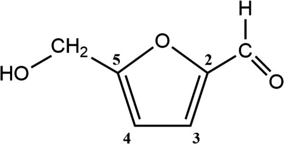
The chemical structure of HMF (5‐hydroxymethyl‐2‐furaldehyde, also named 5‐hydroxymethyl‐2‐furfural, 5‐hydroxymethylfurfural, hydroxymethylfurfural, or 5‐hydroxymethylfurane‐2‐carbaldehyde) is depicted in Figure 1.

Figure 1.

Chemical structure of HMF

HMF has the CAS number 67‐47‐0, the molecular formula C₆H₆O₃, and the molar mass 126.11 g· mol⁻¹. It is a colourless solid with a melting point of 32–35°C and a density of 1.21 g·cm⁻³.

HMF is a degradation product of hexoses and is present in numerous food items containing carbohydrates, e.g. milk, fruit juices, dried fruits, bread, and honey. There are two chemical mechanisms through which HMF can be formed from hexoses: (1) through acid‐catalyzed cyclisation with subsequent loss of water, and (2) through formation of a Schiff base with an amino acid, followed by tautomerisation to an 1,2‐enaminol with subsequent hydrolysis to a 3‐deoxyosone and cyclisation. Disaccharides and higher sugars containing hexoses can be hydrolysed to monosaccharides and therefore also lead to the formation of HMF.

The acid‐catalyzed formation of HMF from mono‐ and disaccharides has first been shown by Düll (1895). It is believed to start from fructose as depicted in Figure 2. Glucose and other hexoses can also feed into this pathway leading to HMF, because they can isomerize to fructose.

Figure 2.

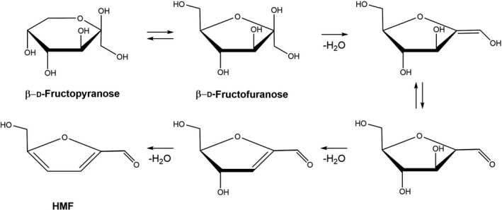
Proposed mechanism of dehydration of fructose to HMF (simplified scheme taken from Yang et al., 2019)

• Carbohydrates are depicted using the Haworth projection.

With respect to mechanism (2), Maillard (1912) first reported that HMF was a product of the reaction of glucose with the amino acid lysin (Maillard, 1912). For a depiction of the detailed mechanism, see Capuano and Fogliano (2011).

Honey is particularly rich in carbohydrates: depending on the source of the nectar, it contains 31–44% fructose, 23–41% glucose, 0.2–7.6% sucrose, 3–16% other disaccharides, and 0.1–4% higher sugars (Ball, 2007). The very low content of amino acids in honey of about 0.1% of the dry matter (Ball, 2007), the acidic pH values of 3.4–6.1 and recent studies by Yang et al. (2019) suggest that HMF is formed in honey primarily through the acid‐catalyzed successive dehydration of fructose according to the scheme depicted in Figure 2. The concentration of HMF in fresh honey is very low to undetectable (Bogdanov et al., 1999) but increases markedly during processing such as heating or long‐term storage (see Section 1.1.4.3). HMF is therefore used as a marker for fresh and unprocessed honey.

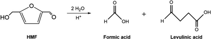
HMF is a stable compound under normal conditions and has been reported to decompose to formic acid and levulinic acid (see Figure 3) only at high temperature and very low pH. Therefore, decomposition of HMF is considered unlikely to take place to a significant extent in honey or bee feeds (Bailey, 1966).

Figure 3.

Decomposition of HMF

HMF can chemically react with amino and thiol groups of proteins due to its aldehyde group and is prone to biotransformation. The aspects of chemical reactivity and metabolism of HMF are considered in Section 3.1.1.

1.1.4.3. Concentration of HMF in honey and various bee feeds

Honey is the natural feed for honey bees when no nectar from flowering plants is available. When stored under natural conditions within the hive, concentrations of HMF in honey are very low (Bogdanov et al., 1999; Krainer et al., 2016). For example, HMF contents of fresh honey from Italy, Turkey, and India were 1.23–5.95, 0–11.5, and 0.15–1.70 mg/kg, respectively (reviewed by Shapla et al., 2018). Heating or improper storage can lead to considerably higher HMF levels. For example, when different honey samples were heated to 100°C for 1 min, the HMF concentration increased from 3.9 to 10.1 mg/kg (Tosi et al., 2001). Karabournioti and Zervalaki (2001) found that the increased levels of HMF in honeys of several botanical origins kept at various temperatures for 24 h were correlated with the temperatures Shapla et al. (2018) reviewed HMF concentrations of honey samples from 29 countries after storage for up to three years at temperatures up to 30°C; there was a clear trend for increasing HMF levels with longer storage times and higher storage temperatures, the highest value being 1,132 mg/kg in a Malaysian honey kept at 30°C for more than 2 years. The importance of time and temperature for the level of HMF was confirmed in a controlled study with coriander honey (Kamboj et al., 2019), but the authors emphasize that other factors such as pH, water content, sugar profile, presence of organic acids and floral source of the honey may also have an effect. The multifactorial reasons for HMF formation may explain the highly variable HMF levels reported in the review by Shapla et al. (2018).

In order to facilitate winter feeding of bee colonies from which honey has been removed, bee feed is given. For example, a concentrated solution of the disaccharide sucrose is a suitable bee feed, because sucrose does not lead to digestive problems and is less likely to crystallise than honey. Moreover, HMF is not formed from unhydrolyzed sucrose (Simpson et al., 1968). To further reduce the problem of crystallization at low temperatures, the presence of fructose is beneficial for bee feeds, such as in high fructose corn syrup (HFCS) and inverted sugar syrup. HFCS is produced from corn starch, which consists of amylose and amylopectin that are polysaccharides containing only glucose moieties. After acid‐catalyzed or enzymatic degradation part of the glucose is transformed to fructose. A complex fractionation and combination process can be used to obtain mixtures with various amounts of fructose, e.g. HFCS‐42 (42% of fructose) and HFCS‐90 (90% of fructose).

Inverted sugar syrup is a mixture containing glucose and fructose. It is obtained from sucrose through acid‐ or enzyme‐catalyzed hydrolysis. Additional fructose can be added to further hinder crystallization. Sometimes inverted sugar syrup is acidified with organic acids (i.e. citric, oxalic, acetic or lactic acid) which are supposed to improve its suitability as bee feed for the winter (Ceksteryte and Racys, 2006).

All commercially available bee feeds contain either sucrose or mixtures of glucose and fructose at different proportions. Some other sugars, such as mannose, galactose and lactose have been found to be harmful to honey bees (Barker and Lehner, 1974; Brodschneider and Crailsheim, 2010) and are therefore not used as supplemental feeding. The physicochemical properties of suitable feeds are mostly determined by the water content. Basically, there are four types of commercial bee feeds: Syrup, fondant, candy, and dry sugar. The water content of syrup may vary from 50% down to a few percent, and its consistency accordingly from a solution to a liquid gel or paste. Sugar syrup is commonly used from spring to autumn. When temperatures fall below 10°C, syrups may freeze and must be replaced by bee fondant or candy or granular sugar, all three of which can be consumed by honey bees throughout the winter. During the freezing of syrup HMF is concentrated in the liquid portion, which is the only one accessible to the bees (Wilmart et al., 2011). Thus, syrup crystallization may lead to higher HMF exposure.

Fondants and candies are prepared from an aqueous sucrose solution by gently evaporating most of the water and letting the sugar solidify with stirring to avoid crystallization; the temperature of cooking determines the consistency of the final product. Fondant is softer than candy, it is squeezable and pliable like dough because it contains more residual water. Sometimes, fondants are referred to as ‘soft candy’. With respect to dry sugar, pure granular sucrose (‘white sugar’) from sugar beets or sugar cane appears to provide the least risk to bees for digestive problems, whereas raw, brown, and waste sugars may contain other carbohydrates or contaminants and are not suitable (Somerville, 2014).

In conclusion, commercial bee feeds may contain varying levels of HMF, depending on the conditions during their production and use. Several parameters are known to influence the rate of HMF formation during preparation of bee feeds, the most important being the type of sugar and the pH, the temperature, the water activity, and the concentration of divalent cations of the media (Capuano and Fogliano, 2011).

1.1.4.4. Analytical methods for detection and quantification of HMF

The International Honey Commission (IHC, Bogdanov, 2009) recommends three analytical methods for the determination of HMF. These comprise two spectrophotometric methods, named after Winkler (1955) and White (1979), and one chromatographic method, using HPLC.

In the Winkler method, the HMF is reacted with p‐toluidine and barbituric acid to form a dye the absorbance of which is measured at 550 nm. Reaction only with p‐toluidine but not barbituric acid serves as reference. The major drawback of the Winkler method is the use of p‐toluidine, which is a carcinogenic compound.

The White method measures the absorbance of HMF at 284 nm directly, using as reference another aliquot to which sodium bisulfite has been added in order to convert HMF to a derivative which no longer exhibits absorbance at 284 nm. Refinements of this method account for UV‐absorbing matrix constituents (Kozianowski, 2016).

The HPLC method is based on the report by Jeuring and Kuppers (1980). Briefly, the diluted and filtered honey sample is analysed on a reverse phase HPLC column using isocratic elution and UV detection at 285 nm. Quantitative determination is carried out using external standardization.

The three methods were tested by the IHC with three honey samples covering the HMF concentration range of 4 to 40 mg/kg (Bogdanov, 2009). All three methods yielded comparable results for the samples with 40 and 20 mg/kg, and only small differences between the methods were observed at the lowest HMF levels. The reproducibility of the HPLC method and the White method were better than that of the Winkler method. Likewise, Zappalà et al. (2005) reported that the HPLC and the White methods give similar results for the HMF content of various unifloral honeys, whereas the Winkler method gave higher values. Truzzi et al. (2012) compared the HPLC and the White method for the determination of HMF in unifloral honey and honeydew samples with a HMF content of less than 4 mg/kg. For honey samples with an HMF content in the range of 1–4 mg/kg, both methods were suitable but the HPLC method was superior to the White method with respect to precision.

In general, the HPLC method appears to be more suitable for the determination of HMF than the spectrophotometric methods, in particular for samples containing matrix constituents which may interfere with the photometric measurement of HMF but are separated from HMF in the HPLC method (Kozianowski, 2016).

Various modifications of the HPLC method have been reported, including sample preparations using liquid‐liquid extractions (Chen et al., 2019). In addition, methods using high‐performance thin layer chromatography, gas chromatography, and micellar electrokinetic capillary chromatography have been developed for analysing HMF in honey (cited in Chen et al., 2019), but these methods are not commonly used. For a complete list of all methods for the determination of HMF in food see Morales (2009).

1.1.4.5. Legislation

HMF is currently not regulated under Directive 2002/32/EC ⁴ on undesirable substances in animal feed and also not listed in the Annex to Commission Regulation 68/2013 ⁵ on the requirements for feed hygiene.

Article 15 of Regulation 178/2002 ⁶ stipulates that feed shall not be placed on the market or fed to any food‐producing animal if it is unsafe e.g. if it has adverse effects on human or animal health.

2. Data and methodologies

The draft Opinion underwent a public consultation from 3 December 2021 to 10 February 2022. The comments received and how they were taken into account when finalising the scientific Opinion are available in Annex A to this scientific Opinion.

2.1. Collection and appraisal of data from public literature

In preparation of the present mandate, a call for a procurement for a literature search and review was launched with the aim to identify, collect and evaluate literature related to the effects on HMF in bee feed. A final project report was delivered in July 2020, and was published on 7 August 2020 (NFI‐DTU, 2020). Briefly, in the outsourced work four search strings related to (1) chemical identification, characterisation and formation, (2) occurrence in bee feed and honey, (3) toxicokinetics and (4) toxicity were designed to identify and collect potentially relevant studies in several databases. Results from the search was then evaluated regarding the potential relevance for the present opinion applying inclusion/exclusion criteria for the studies (for details see NFI‐DTU, 2020). No time limit was applied for this search. The total number of publications identified per research field and those identified as potentially relevant by the contractor were as follows (total number/potentially relevant): Chemical identification, characterisation and formation (3,862/55), occurrence in bee feed and honey (37/14), toxicokinetics (221/15), toxicity (500/8). The report contains summary tables (as annexes) containing all abstracts that were screened together with an evaluation of their relevance and listing the key points of the individual publications. The abstracts proposed as potentially relevant in the report were then screened by the WG members, and by applying expert judgement, the associated studies were considered as part of the assessment if relevant. In addition to the systematic search for retrieval of relevant literature, a ‘forward snowballing’ approach was applied by all WG members (see Jalali and Wohlin, 2012) to obtain further any relevant information.

2.2. Methodology – Occurrence data submitted to EFSA

Following the European Commission mandate to EFSA, a call for annual collection of chemical contaminant occurrence data in food and feed, including HMF, was issued by the former EFSA Dietary and Chemical Monitoring Unit (now Evidence Management Unit) in December 2010 with a closing date of 1 October of each year. European national authorities and similar bodies, research institutions, academia, food business operators and other stakeholders were invited to submit analytical data on HMF in feed. The data submission to EFSA followed the requirements of the EFSA Guidance on Standard Sample Description (SSD) for Food and Feed (EFSA, 2010). Occurrence data were managed following the EFSA standard operational procedures (SOPs) on ‘Data collection and validation’ and on ‘Data analysis of food consumption and occurrence data’.

The raw data on occurrence from EU MS are available at the EFSA Knowledge Junction community on Zenodo. ⁷

2.3. Feed consumption in honey bees

Honey bees consume nectar and honey to cover their carbohydrate requirements, during their development as larvae and later for their daily activities as adults. Food consumptions in honey bees have been extensively reviewed by EFSA through a systematic and narrative reviews (EFSA, in preparation).

As adults, bees consume nectar/honey during their entire life to achieve their various tasks in the hive and, thereafter, outside the hive, as forager bees. The activities that are the most expensive in terms of energetic costs are those related to foraging and thermoregulation for the brood (during the development of the colony from spring to autumn) and the nest (in winter). Indeed, bees consume nectar/honey to maintain the temperature (via thermoregulation) of the brood at about 34°C and the nest/bee nucleus at 5–8°C in the periphery and 15–20°C in the centre. Those activities require 32–128 mg sugar per day (foraging), 34–50 mg sugar per day (brood thermoregulation) and 8.8 mg sugar/bee per day (nest thermoregulation) (Rortais et al., 2005; EFSA PPR Panel, 2012). The estimate of an uptake of 8.8 mg sugar/bee per day is an average value obtained from a scenario that assumes the consumption of 20 kg of honey by 20,000 bees located in temperate EU regions during a 3‐month winter period (Rortais et al., 2005) and is therefore used for the exposure assessment in the present opinion. Notably, this consumption estimate does not take into account any natural variations (periods of low consumption alternated with periods of high consumption in relation to external temperature variations) that might occur during this long period across the various climatic regions found in EU. As bee feed is mainly given during the cold season, a default consumption value of 8.8 mg sugar/bee per day (nest thermoregulation) has been chosen as most appropriate for the exposure assessment. On a gram basis, which is used throughout this opinion, the caloric equivalents of the carbohydrates sucrose, glucose and fructose are virtually identical (about 4.0 kcal or 16 kJ per gram).

Standard feed consumption levels (i.e. doses and concentrations) in laboratory settings were established by Tosi et al. (2021), thus allowing to set up a toxicological reference point. They performed a ring‐test involving seven different laboratories in Europe and USA that investigated the feed consumption of worker bees in laboratory conditions and found that that the mean consumption of sucrose (consumed as a 50% aqueous solution) was 13 (day 1–10), 14 (day 21–30) and 12 (day 31–40) mg sucrose/bee per day, respectively. An average value of 13.5 mg/sugar per bee per day has been identified as most appropriate default consumption value for establishing exposures in toxicity tests to be able to derive doses from the concentrations given.

2.4. Methodology for exposure assessment

The exposure of workers to HMF for the different scenarios was estimated by using the concentration data provided by the data provider from MS (Data set A) and industry (Data set B). The CONTAM Panel considered that only chronic dietary exposure had to be assessed. In the absence of measured consumption data for worker bees default values have been used (see Section 3.3).

2.5. Methodology for risk characterisation

The risk characterisation was carried out by comparing the exposure estimates from the different scenarios with the reference point for bee toxicity. All the principles in the EFSA guidance on risk assessment for bees and pollinators (EFSA, 2013a,b) were followed.

3. Assessment

3.1. Hazard identification and characterisation

3.1.1. Toxicokinetics

No information is available on the toxicokinetics, i.e. the absorption, distribution, metabolism and excretion of HMF, in honey bees or other insects. However, a few toxicokinetic studies of HMF in rodents and humans have been conducted (reviewed in Abraham et al., 2011; Farag et al., 2020). For example, Godfrey et al. (1999) reported that the urine of rats and mice collected for 48 h after oral administration of ¹⁴C‐labelled HMF at doses ranging from 5 to 500 mg/kg body weight (bw) contained 60–80% of the administered dose, while 10–25% were excreted with the faeces. The studies on the tissue distribution as well as on the excretion suggest that HMF is rapidly and completely absorbed, metabolised and excreted after oral ingestion by rodents.

The major metabolic pathways of HMF in mammals are depicted in Figure 4.

Figure 4.

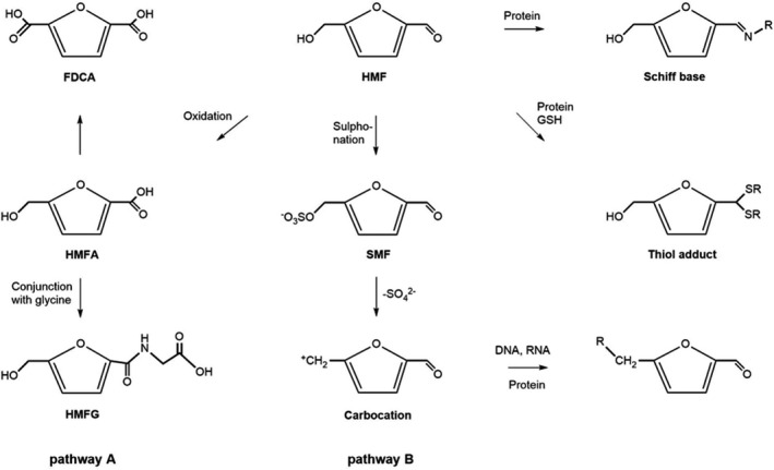
Major metabolic pathways and reactivity of HMF and its metabolites. R represents biomolecules capable of covalent binding through their amino or thiol groups

Pathway A involves oxidation of the aldehyde group to yield 5‐hydroxymethyl‐2‐furoic acid (HMFA), followed by conjugation of HMFA with the amino acid glycine to give 5‐hydroxymethyl‐2‐furoyl glycine (HMFG), or further oxidation to 2,5‐furane dicarboxylic acid (FDCA, Figure 4). HMFA, HMFG, FDCA and traces of other metabolites were also detected in human urine after consumption of HMF‐containing fruit juices (Pryor et al., 2006; Abraham et al., 2011 and literature cited therein).

Another metabolic pathway of HMF (pathway B in Figure 4) comprises the conversion of HMF to 5‐sulfoxymethylfurfural (SMF) via sulfonation of the hydroxymethyl group. SMF represents an allylic sulfuric acid ester which readily splits into a sulfate ion and an electrophilic carbocation capable of covalent binding to nucleophilic sites of proteins and nucleic acids and thereby eliciting cytotoxic and mutagenic effects. The formation of SMF has been demonstrated in mice and humans.

Finally, the aldehyde group of HMF has been shown to react directly, i.e. without metabolism, with free amino groups and/or thiol groups of proteins, thereby forming Schiff bases or thiol adducts, respectively (Figure 4). This may contribute to the covalent binding of radioactivity observed in the kidney, bladder and liver of rodents after oral ingestion of ¹⁴C‐labelled HMF (Godfrey et al., 1999).

Although no studies on the metabolism of HMF in honey bees or in other insects have been conducted, it is of interest to note that the genome of honey bees has a smaller number of genes for the metabolism of xenobiotics relative to other insect genomes (Berenbaum and Calla, 2021, and literature cited therein).

In addition to the lack of information on the metabolism of HMF in honey bees, it is unknown if HMF can interact with their gut microbiota. Effects of HMF on the human gut microbiome have been reported (Aljahdali and Carbonero, 2019). Because the gut microbiota is important for the health of honey bees, exposure to HMF might change their composition with a negative health impact. The issues of HMF toxicokinetics in honey bees and effects on their gut microbiome require investigation.

3.1.2. Toxicity

The available laboratory toxicity and field studies with HMF are presented in the following Sections 3.1.2.1 and 3.1.2.2.

3.1.2.1. Experimental studies in honey bees

Bailey (1966) gave groups of 30 caged honey bees (Apis mellifera) taken from the same colony various sugar products dissolved in 60% sucrose syrup and measured the time until half the bees in a cage had died. The sugar products comprised sucrose hydrolysed with acids under various conditions, or with the enzyme, invertase. Honeys of different age and the degradation products HMF, levulinic acid and formic acid were also tested. Whereas sucrose hydrolysed with invertase was found to be nontoxic, bees fed carbohydrates hydrolysed with mineral or organic acids developed severe dysentery and died within a few days. Likewise, bees receiving unrefined sugar, heated honey, HMF, levulinic acid or formic acid died early. At the tested concentration of ca. 80 mM (corresponding to 1% HMF), the three degradation products were equally toxic to bees. HMF became harmless when diluted to 10 mM. Testing a mixture of HMF, levulinic acid and formic acid did not suggest that these compounds have a combined effect. Bees fed 8‐year‐old honey became more dysenteric compared with those fed fresh honey or syrup. The CONTAM Panel concluded that this study could not be considered for the present assessment as a concentration/dose response curve could not be established from this paper.

In two independent experiments carried out in 1973 and 1974, Jachimowicz and El Sherbiny (1975) fed groups of 500 (100 animals per test group in five replicates) newly emerged (0–3 days old) Carniolan worker bees (Apis mellifera carnica) for 20 days with ‘synthetic’ solutions made of glucose, fructose and sucrose (7:7:1 by weight) and 50% water to which HMF was added at concentrations of 0, 30, 150 and 750 mg/kg. The pH of the feeding solutions was adjusted to 3.9 by adding citric acid. In a separate experiment, it was shown that the addition of citric acid did not have an effect of the toxicity of the solution. A commercial invert sugar solution with identical sugar composition and 30 mg HMF/kg was also tested. Mortality rates reported here are the mean values from the two independent experiments which differed only marginally. A concentration of 30 mg HMF/kg did not lead to a significantly increased mean mortality rate (15%) as compared to the control (12.5%) after 20 days. In contrast, mean 20‐day mortality rates were clearly increased with concentrations of 150 mg/kg (58.7%) and 750 mg/kg (98.8%). The commercial solution exhibited the same mortality rate as the synthetic solution with the same HMF level.

Leblanc et al. (2009) fed triplicate groups of 100 caged freshly emerged worker bees (Apis mellifera ligustica) with either commercially available HFCS‐55 containing 57 mg/kg HMF or with HFCS‐55 spiked with pure HMF to produce final concentrations of 100, 150, 200 and 250 mg/kg HMF. The caged trials were recorded in multiples of four. Syrup consumption during the first 3 days was found to range between 50 and 70 mg per bee. Drinking water was supplied ad libitum. However, when the water supply expired without being replenished, more syrup was consumed, and the mortality increased dramatically. A mortality of 50% was reached in the 150 mg/kg group after 19 days. A comparison of 26‐day mortality showed that mortality did not differ significantly between the 57, 100, 150 and 200 mg HMF/kg groups while it was significantly higher in the 250 mg/kg group (more than 90% mortality at mean). The CONTAM Panel noted that in this study, no negative control (i.e. HMF‐free bee feed) was tested. Feed consumption was only measured on days 1–3 and days 5–26 and figures for consumption have not been reported. Bees have consumed more syrup because of lack of water occurring in some cages (where water supply expired without being replenished) leading to high consumption of HMF containing syrup and dramatically increased mortality in these cages. Actual figures (mean and standard deviation) for survival rates at day 26 were not reported. The percentage survival rates (numerical figures were not reported but only presented in a column chart) were clearly below 25% at all concentrations. Taking all these uncertainties with regard to the results and their presentation into account, the CONTAM Panel decided not to consider these results further in this assessment.

Smodiš Škerl and Gregorc (2014) fed caged worker bees (approximately 50 animals per cage, in five replicates), kept at 28°C and a relative humidity of 60%) with commercial sugar candies for 27 days purchased in Slovenia and a home‐made candy in order to investigate effects on bee longevity. Some of the candies contained high amounts of HMF. The candies were ‘MedoPip Standard’ (914.6 mg HMF/kg), ‘Medopip Plus’ (437.0 mg HMF/kg); ‘Apimel’ (58.3 mg HMF/kg), the ‘home‐made sugar candy’ (< 10.0 mg HMF/kg) and ‘Stimulans’ candy (< 10.0 mg HMF/kg). HMF concentrations were determined by HPLC. The longest worker survival (27 days) was found with the candies with lowest HMF levels namely ‘Apimel’, ‘home‐made sugar candy’ and ‘Stimulans candy’ while feeding with ‘Medopip Standard’ and ‘Medopip Plus’, the candies with the highest HMF, resulted in shorter life spans (24 and 20 days, respectively). Since the study only provides information on longevity but not on comparative survival of bees at the different doses at the same time points which would allow establishment of a concentration/dose response, the CONTAM Panel decided that it cannot be used for characterising the risk of HMF to bee health.

In order to assess the effect of HMF of mortality of larvae, Krainer et al. (2016) fed groups of artificially reared larvae with diets containing 50% royal jelly and 50% aqueous sugar solutions with varying fructose, glucose and yeast extract concentrations to fulfil the different demands of young and old larvae. HMF was added at nominal concentrations of 0, 5, 50, 750, 5,000, 7,500 and 10,000 mg/kg and the spiked diet fed for 6 days. For the control group, 12 replicates and for the test groups seven replicates with one plate containing 48 larvae each were tested. Larvae were kept at 34.5°C and 96% humidity. Mortality was assessed on day 7 and 22 of the observation period. On day 7, mortality of groups receiving 0, 5, 50, 750, 5,000, 7,500 and 10,000 mg/kg HMF was 9% (standard error (SE) ±1.19), 6.9% (±1.5), 10.1% (±1.77), 6.8% (±1.38), 52.4% (±2.72), 100% and 100%, respectively. The corresponding figures for the mortalities measured on day 22 were 28.1% (±0.019) at 0 mg/kg, 26.4% (±2.60) at 5 mg/kg, 30.2% (±0.027) at 50 mg/kg, 32.1% (±0.026) at 750 mg/kg and 87.5% (±0.018) at 5,000 mg/kg, respectively. The authors concluded that increased mortality was only reported in groups fed diets containing HMF concentrations higher than 750 mg/kg and that a concentration of 7,500 mg/kg caused a mortality of 100%. Experimental of LC₅₀ values HMF for larvae of 4,280 mg/larva (day 7) and 2424 mg/kg (day 22) were determined. Using a total uptake of 170 µl feed, the calculated LD₅₀s for larva were 778 µg HMF/larva (day 7) and (day 22) 441 µg HMF/larva.

In a second experiment, aimed at comparing HMF toxicity in larvae with adult animals, triplicate groups of 48 freshly hatched adult worker bees were feed sucrose solutions (50% w/v) containing either 0, 2,000, 4,000 and 8,000 mg HMF/kg. On day 7, mortalities in the different test groups were 0.7% (SE ± 0.470) each for the control group and the 2,000 mg/kg group, and 3% (± 0.985) and 5% (± 1.26) in the 4,000 and 8,000 mg/kg group, respectively. On day 22, the mortality of the control group was 6.7% (±1.44) and that of the 2,000 mg/kg group was 67% (±2.71). A 100% mortality was already reached at day 20 in the 4,000 mg/kg group and at day 15 in the 8,000 mg/kg group. For adult worker bees, an LC₅₀ values of 82,778 mg HMF/kg (day 7) and 1,843 mg HMF/kg (day 22) were derived applying regression analyses. An LD₅₀ was not calculated because feed consumption of worker bees was unknown. The authors concluded that on day 7 (after 6 days of treatment), larvae are much more sensitive towards HMF compared to adult worker bees; however, on day 22, adults show a lower LC₅₀ (1,843 mg HMF/kg) as compared to larvae (2,424 mg HMF/kg), indicating a higher sensitivity of adult animals towards HMF.

Gregorc et al. (2020) fed groups of 70 caged newly emerged (0–24 h) Carniolan worker bees (Apis mellifera carnica) in five replicates for 50 days with commercial bee candy (Apifonda, Südzucker, Mannheim, Germany, 83% sucrose, 5.5% dextrose, 3.0 fructose, 2,5% maltose and 8.0% higher saccharides, approx. 90% dry matter) to which nominal concentrations of 0, 100, 500, 1,000 and 1,500 mg HMF/kg were added to assess HMF‐induced mortality rates. The bees were kept in incubators at 28°C and 65% relative humidity. Daily food consumption was recorded. For immunohistochemical analyses (in situ cell death detection kit (ISCDDK)), groups of 50 animals were given the same test concentrations as in the mortality study, and three animals were randomly sampled from each group at days 5, 10, 15 and 20 and their midguts removed. For the analysis of cell death, about 300 cells from each of the three bees were counted.

After 15–30 days of exposure, an increased mortality rate was observed that was clearly time and HMF concentration dependent. In Table 1, the % survival rates with standard deviations of the control and substance groups at the different time points in this experiment are presented in detail.

Table 1.

Effects of intake of HMF on survival rates in worker bees^(a)

Days	Apifonda		Apifonda + 100 mg/kg HMF		Apifonda + 500 mg/kg HMF		Apifonda + 1,000 mg/kg HMF		Apifonda + 1,500 mg/kg HMF
	% survival	SD	% survival	SD	% survival	SD	% survival	SD	% survival	SD
5	99.7	0.3	99.2	0.5	99.6	0.5	99.4	0.6	99.5	0.4
10	98.8	0.2	97.5	0.7	98.3	0.4	97.5	0.2	97.8	1.2
15	97.6	0.4	95.5	0.9	96.9	1.0	96.1	1.1	91.9	2.3
20	91.7	6.2	88.6	6.0	87.7	7.4	87.7	6.2	75.0	11.6
25	70.9	6.6	65.7	8.3	57.6	9.9	49.6	18.1	37.8	13.6
30	42.4	10.7	33.0	11.1	27.7	10.4	18.0	6.0	11.9	4.3
35	21.9	4.5	10.5	0.9	9.0	1.0	4.4	1.1	3.4	2.3
40	11.9	3.8	2.6	0.7	5.4	0.8	0.9	1.2	0.9	0.4
45	4.5	1.8	1.1	0.5	3.2	0.5	0.0	0.0	0.0	0.0
50	0.8	0.7	0.0	0.0	1.0	0.8	0.0	0.0	0.0	0.0

HMF: Hydroxymethylfurfural; SD: standard deviation.

^aData were kindly provided by Ales Gregorc.

During the first 2 weeks of treatment, sublethal effects on midgut cells were observed i.e. ISDDK‐positive midgut epithelial cells indicative of apoptosis. A hypertrophic enlargement of the digestive cells was seen with the first 5 days in HMF‐fed bees. After 10 days of HMF treatment, numerous affected cells were shed into the midgut lumen, as evidenced by observable apoptotic cell death in the apical region of midgut. Between day 10 and 15, increased cell death rates were observed in the 1,000 and 1,500 mg/kg treatment groups, resulting in the shedding of dead cells from the epithelium into the midgut lumen, followed by typical necrotic deletions. Notably some variations in pathological cell death were also observed in the 500 mg/kg group.

The authors concluded that the bees were sensitive to changes found in the midgut tissue already at sublethal HMF concentrations. HMF feeding and its potential detrimental effect can result in higher bee mortality which was monitored 14 days after caged bees were exposed to HMF. It was found that HMF has a dosage‐dependent cytotoxic effect on honey bee digestion; both sublethal and subclinical changes to the midgut occur at the cellular level before bees eventually die from high doses.

The CONTAM Panel noted that the concentration‐related increase seen in ISCDDK positive cells observed in particular at high doses after 5 days was not seen anymore at later time points, likely because of the progressing severity of cell lesions in the midgut which cannot be detected with such a rather sensitive method.

Frizzera et al. (2020) fed groups of 25 bees with sugar syrup (glucose 61%, fructose 39%) to which different concentrations of HMF were added (0, 50, 100, 200 and 400 mg/kg). At these concentrations, no effect of HMF on bee health was found, even in the presence of the mite Varroa destructor, a common stressor in honey bees. In another experiment, the survival of bees fed with sugar syrup (2:1) alone and with syrup containing 100,00 mg HMF/kg was compared, using 30 bees per group and three replicates. The high concentration of HMF was used because previous experiments had shown that 6,000–14,000 mg HMF/kg are formed in home‐made sugar syrups at a pH of 2 after 30–40 min of boiling, which is standard practice in when preparing bee syrups. A 100% mortality rate was reached after 14 days in the HMF group, while more than 85% of control bees were still alive. The CONTAM Panel noted that the survival rates of bees fed with various HMF concentrations in the first experiment were not different from control. In the second experiment only one very high dose was tested and no dose response curve can be derived. Therefore, this study could not be used for the risk characterisation.

A non‐peer‐reviewed study (Lüken and Ohe, 2016) aimed at investigating the effects on HMF on bee mortality. In a first trial carried out in summer, groups of bees (Apis mellifera carnica) received sugar solutions via a syringe containing nominal concentrations of 0, 40, 120, 240, 480, 960, 1,920 and 3,840 mg HMF/kg, respectively, for 30 days. The number of bees in the control group was 200, that in the test groups was 80. Bees were kept in a climate cabinet at 25°C ± 2°C and at a relative humidity of 60%. Average feed consumption (all groups) was 15.55 mg/bee per day. Cumulative mortality after 35 days was 46.25% in the control and 35.50% in the highest dose test group (numerical values for other groups not reported). In a second trial carried out in autumn, with identical test design except for an increased temperature of 33°C, average feed consumption in the different groups was 22.9 mg/bee per day. Cumulative mortalities after 30 days were 18.5, 13.75, 21.25, 18.75, 27.5, 45.0, 77.5 and 97.5%, respectively. The CONTAM Panel noted that this study was not peer reviewed and there were considerable discrepancies between the results of the two independent trials which could not be explained by the authors.

3.1.2.2. Field studies using honey bee colonies

Van der Zee and Pisa (2010, 2011) provided some evidence of bee mortality related to cases of high concentrations of HMF in a certain batch of a common bee feed used in the Netherlands. They collected data from 1,568 beekeepers after the 2009–2010 feeding season, in which an increase in mortality of bee colonies compared to previous years was observed. The Netherlands Centre for Bee Research (NCB) ran an investigation on the largely used inverted sugar syrup ‘Saint Ambrose Syrup’. The syrup batches, produced by De Bijenhoff, had high concentrations of HMF of up to 475 mg/kg and of glucose up to 32 mg/kg as compared to the low contents of sucrose (1–13 mg/kg). The producer of Saint Ambrose Syrup provided no information on HMF content and gave a concentration of 33 mg/kg for sucrose. The authors concluded that the high amounts of glucose were responsible for crystallisation of the feed which caused bees to starve, and HMF for the poisoning of honey bees. The combination of these factors increased the bee annual disease from an average of 23.1% in the previous years to 29.1% for the 2009–2010 winter season.

Kozianowski (2016) carried out a field study in 2012–2013 by adding pure HMF in concentrations between 20 and 150 mg/kg to a fructose/sucrose‐based commercial syrup. A total of 60 young colonies in six feeding groups were located in different but climatically comparable locations in the Jagst Valley (in northern Baden–Württemberg). The six groups were fed Apiinvert with 7, 20, 40, 80 or 150 mg HMF/kg syrup, or a 60% aqueous solution of pure sucrose (control) over a period of 14 days in late August/early September. The level of HMF in all feeds except the control increased during the feeding period on average by 20 mg/kg feed, probably due to the warm weather. When the feed stored in the combs was analysed after the winter, the HMF levels in the spiked Apiinvert feeds had dropped to 16–36 mg/kg. One colony exposed to 80 mg/mg did not survive due to loss of the queen. Another colony receiving 20 mg HMF/kg was recorded with high levels of faeces and a high number of deaths. The authors consider those two cases as typical individual events which cannot be attributed to HMF exposure and emphasise that no other adverse effects were found in the colonies even with the highest dose of HMF. From this study, it was demonstrated that HMF concentrations up to 150 mg/kg in a fructose/sucrose‐based feed syrup (Apiinvert) is well tolerated by bee colonies under practical conditions.

Semkiw and Skubida (2016) conducted a study on five different syrups as bee feeds in the winter of 2012–2013 and 2013–2014 with respect to feed consumption, colony strength and development dynamics, honey yield from spring flow and bee mortalities. The feeds analysed where three commercial starch syrups (Apifood ‐ from Poland, Apikel 20‐ from Germany, Apifortune ‐ from France), one commercial inverted sucrose syrup (Apiinvert ‐ from Germany) and a home‐made syrup (sucrose to water ratio 5:3). HMF levels in the feeds were not analysed in the study, but stated by the manufacturers as < 40 mg/kg for Apifood and < 20 mg/kg for Apikel 20. The authors assumed that the HMF content did not change with time due to the controlled temperature (15°C) during feed storage (2 months) and to the cold climate of the region. No crystallisation of the starch or inverted sucrose syrups occurred during the experiment and no significant differences in the condition of bee colonies were noted before or after overwintering, and during spring development. The authors conclude that HMF levels in bee feed not exceeding 40 mg/kg are safe for bee colonies.

3.1.3. Mode of toxic action of HMF in bees

A frequent cause of death of honey bees is called ‘dysentery’, which for bees means defecation inside the hive due to an excess amount of faecal matter in the gut. Bees retain 30–40% of their body weight in their intestine, and if the time between cleansing flights is too long, they will void inside the hive. This situation can arise for healthy bees in very cold and long winters, especially if their feed contains high amounts of indigestible solids, in particular ashes, the amount of which varies between different types of honey. Thus, dysentery is not necessarily a disease but a condition. However, lesions of the bee gut by toxins may also lead to dysentery.

Bailey (1966) observed that HMF caused gut ulceration in worker bees resulting in dysentery. He excluded a crucial role of the HMF breakdown products levulinic acid and formic acid because the amounts of these compounds formed in sugar solutions are too small to explain the mortality. Bailey also doubts that HMF itself is responsible for adverse effects of bee feed, noting that there might be other yet unknown compounds accounting for the toxicity.

Gregorc et al. (2020) stated that the mechanism by which HMF negatively affects bee health or leads to increased mortality is unknown. In their study, next to mortality, they have also investigated the effect of HMF on the midgut as it can be assumed that this is the tissue mainly exposed to HMF. Hypertrophic enlargement of digestive cells was observed as an early effect, followed by apoptotic cell death in the apical region of the midgut villi. With progressing time, the rate of cell death increased, resulting in shedding of dead cells from the epithelium into the lumen of the midgut. In bees exposed to high doses of HMF, apoptosis was followed by necrosis and increased mortality was paralleled by histopathological lesions in the midgut.

3.1.4. Identification of critical effects

3.1.4.1. Acute effects

The CONTAM Panel did not identify studies on acute effects of HMF in bees. However, based on the chronic studies presented in Section 3.1.2.1 even at very high doses HMF did not cause acute toxicity (i.e. mortality) within the first days of exposure (and actually in most cases only after exposure of 15 days or more). Therefore, HMF is considered of low acute toxicity for honey bees.

3.1.4.2. Chronic effects

In Section 3.1.2.2, field studies on the adverse effects of HMF on bee populations are described. In the study from Van der Zee and Pisa (2010, 2011), the colony collapse seen in the Netherlands was attributed to a combination of starvation of bees because of crystallised bee feed and high HMF contents in bee feed. Semkiw and Skubida (2016) found that concentrations of up to 40 mg HMF/kg bee feed had no adverse effects on colonies, and Kozianowski (2016) concluded that feeding of bees with concentrations of up to 150 mg HMF/kg bee feed had no adverse effects on colonies. The CONTAM Panel noted that field studies are more likely to reflect the real situation as compared to laboratory studies with an artificial and standardised setting and with a relatively low number of animals. However, the specific contribution of HMF to potentially adverse effects on bee colonies, and colony collapse is difficult to quantify, e.g. because actual concentrations of HMF in bee feed and doses of HMF taken up by the bees are difficult to quantify. Field studies are also prone to bias because of a series of potential confounders also affecting bee vitality and longevity such as climatic factors, exposure to plant toxins, xenobiotics such as pesticides, diseases or predators. These additional confounders and stressors can be excluded in laboratory studies.

Therefore, the CONTAM Panel decided to use the results of laboratory studies for derivation of a reference point for the toxicity of HMF which are described in detail in Section 3.1.6.1. In all these studies, bee mortality/survival rate was used as an endpoint for assessing the toxicity of HMF and was therefore identified as the critical effect for the present assessment.

The CONTAM Panel considered the studies from Jachimowicz and El Sherbiny (1975), Krainer et al. (2016) and Gregorc et al. (2020) as most appropriate for deriving a reference point for the adverse effect (mortality) of HMF in bees. The data obtained from these studies enabled assessing concentration/dose–response relationships and were suitable for benchmark concentration (BMC) and benchmark dose (BMD) analyses. Therefore, they were considered further in the assessment (see Section 4.4).

The CONTAM Panel notes that none of these studies were fully compliant with existing OECD guidelines on chronic toxicity (OECD, 2016, 2017). However, the study design in the respective studies is considered appropriate and valid with regard to most study parameters (e.g. number of animals/replicates, application of feed, climatic conditions, overall reporting) even if positive controls have not been tested. Notably, mortality has been assessed for an even longer time period than the 10 days requested in OECD 245 i.e. 20 and 22 days in the Jachimowicz and El Sherbiny (1975) and Krainer et al. (2016) studies and even up to 50 days in the Gregorc et al. (2020) study. In all of the three studies, background mortality even at around 20 days of exposure was below the threshold of 15% (set for an exposure of 10 days in OECD 425). Background mortalities from Gregorc et al. (2020) from day 25 onwards exceeded this threshold and the results from these time points were therefore not considered.

Besides the three appropriate studies discussed above, it was noted that the autumn trial in the non‐peer‐reviewed study by Lüken and von der Ohe (2016) could also be used for BMD/BMC analysis. However, background mortalities were slightly above the applied cut‐off criterion of 15%, and no effect was seen in the summer trial, which was otherwise conducted under identical conditions except for temperature (see Section 3.1.2.1). The autumn trial in the Lüken and von der Ohe (2016) study was therefore only used as a reference, adding to the completeness, in the evaluation of the range of BMD/BMC values across available studies, described in the next section.

3.1.5. Concentration/dose response assessment

Table 2 below presents an overview of the study parameters and results from Jachimowicz and El Sherbiny (1975), Krainer et al. (2016) and Gregorc et al. (2020). Information on consumption of bee feed by worker bees has not been presented in any of these studies. Therefore, the HMF concentrations reported have been converted to daily doses per bee using mean values for sugar solution intakes in laboratory studies as described by Tosi et al. (2021). Considering that the length of the above‐mentioned laboratory studies, or the time points at which increased mortality was observed in all three studies was after around 20 days, this was done by using the average intake over the first 20 feeding days as reported by Tosi et al. (accepted) and dividing by half to account for pure sugar consumption. This resulted in an average daily sugar consumption of 13.5 mg/bee per day.

Table 2.

Overview of toxicity studies with worker bees and larvae considered for derivation of BMCs/BMDs for HMF

References	Bees per group	Number of feeding days	sugar/water ratio of bee feed	Number of dead bees per group(a)		Concentration in mg HMF/kg feed	Dose in μg HMF/bee per day	Percentage of mortality/survival with SD/SE as reported in the studies		Derivation of dose
Jachimowicz and El Sherbiny (1975)(b),(c)	500 workers (5 replicates with 100 bees)	20	50/50	Year 1973	Year 1974			Year 1973	Year 1974	Assuming an uptake of 27.0 mg bee feed/bee per day based on default uptake of 13.5 mg sugar/bee per day(a),(g)
				60	65	0	0	12.0	13.0
				70	80	30	0.81	14.0	16.0
				287	300	150*	4.05*	57.4*	60.0*
				496	492	750*	20.25*	99.2*	98.4*
Krainer et al. (2016)(d)	144 workers (3 replicates with 48 bees)	7/22	50/50	7 days	22 days			7 days	22 days	Assuming an uptake of 27.0 mg bee feed/bee per day based on default uptake of 13.5 mg sugar/bee per day(a),(g)
				1	10	0	0	0.7 ± 0.47	6.7 ± 1.44
				1	97	2,000	54.00	0.7 ± 0.47	67.0 ± 2.71*
				7	144	4,000	108.00	3.0 ± 0.985*	100*
				7	144	8,000	216.00	5.0 ± 1.26*	100*
	336/576 larvae (7 replicates with 48 bees, for test groups and for control 12 replicates with 48 bees)	6 (observation at day 7 or 22)	33/77 (Considering average sugar contents of Royal Jelly and home‐ made syrup	30	94	0	0	9.0 ± 1.19	28.1 ± 0.019	Assuming an uptake of 28.3 mg bee feed/larvae per day based on uptake of 28.3 μL bee feed/larvae per day(b),(f)
				23	89	5	0.14	6.9 ± 1.5	26.4 ± 2.60
				34	102	50	1.41	10.1 ± 1.77	30.2 ± 0.027
				23	108	750	21.22	6.8 ± 1.38	32.1 ± 0.026
				176*	294*	5,000*	141.50*	52.4 ± 2.72*	87.5 ± 0.018*
				336*	336*	7,500*	212.25*	100*	‐‐
				336*	336*	10,000*	283.00*	100*	‐‐
Gregorc et al. (2020)(e)	350 workers (5 replicates with 70 bees)	5	90/10	1		0	0	99.7 ± 0.3		Assuming an uptake of 15.0 mg bee feed/bee per day based on a default uptake of 13.5 mg sugar/bee per day(a),(g)
				3		100	1.50	99.2 ± 0.5
				1		500	7.50	99.6 ± 0.5
				2		1,000	15.00	99.4 ± 0.6
				2		1,500	22.50	99.5 ± 0.4
	350 workers (5 replicates with 70 bees)	10	90/10	4		0	0	98.8 ± 0.2
				9		100	1.50	97.5 ± 0.7
				6		500	7.50	98.3 ± 0.4
				9		1,000	15.00	97.5 ± 0.2
				8		1,500	22.50	97.8 ± 1.2
	350 workers (5 replicates with 70 bees)	15	90/10	8		0	0	97.6 ± 0.4
				16		100	1.50	95.5 ± 0.9
				11		500	7.50	96.9 ± 1.0
				14		1,000	15.00	96.1 ± 1.1
				28		1,500	22.50	91.9 ± 2.3
	350 workers (5 replicates with 70 bees)	20	90/10	29		0	0	91.7 ± 0.4
				40		100	1.50	88.6 ± 6.0
				43		500	7.50	87.7 ± 7.4
				43		1,000	15.00	87.7 ± 6.2
				87		1,500	22.50*	75.0 ± 11.6*

HMF: Hydroxymethylfurfural; SD: standard deviation.

*: Considered as significantly different from control by the study authors.

^aPercentage of mortality or survival have been converted to dead bees per group.

^bSE/SD of mortality rates were not reported.

^cValues are mortality rates.

^dValues are mortality rates.

^eValues are survival rates.

^fValue as reported in Krainer et al. (2016).

^gAverage consumption value derived from Tosi et al. (2021).

In Jachimowicz and El Sherbiny (1975), Krainer et al. (2016) and Gregorc et al. (2020), bee mortality or survival was given in percentages with standard deviations. However, it was regarded more appropriate to treat mortality as a quantal response in order to calculate a benchmark concentration/benchmark dose (BMC/BMD) in line with EFSA guidance (EFSA Scientific Committee, 2017). Therefore, results in the papers were first converted to mortality rates (the number of dead bees per test group), and analyses were then performed using the EFSA web tool for BMD analysis, which uses the R‐package PROAST, version 69.0, for the underlying calculations. Table 2 provides an overview on the study parameters and results of the toxicity studies.

For conversion of reported HMF study concentration to doses a daily sugar dose for larvae has been derived from information on the total daily intake and dry matter of syrups. In Krainer et al. (2016), an actual total intake of bee feed by larvae over 6 days of 170 µL (28.3 µL/larva per day) was reported. Due to lack of data regarding the mix solutions (50% ww of sugars water solutions and 50% ww of royal jelly), more detailed information were taken from Aupinel et al. (2005). As described by Aupinel et al. (2005) and mentioned in Krainer et al. (2016), three typologies of syrups were used as part of the 6‐day feeding protocol, based on larvae stage development: day 1–2 solution A (dry matter 29.55%), day 3 solution B (dry matter 33.05), day 4–6 solution C (dry matter 36.55). Using the dry matter average for these sugar solutions (33%), a daily sugar consumption of 9.3 mg/larvae per day was calculated, and used for conversion of concentrations to daily HMF doses per larva. In this process, an average density for sugar solutions equal to 1 was applied to enable consideration of feed uptake on a weight basis (mg bee feed/larva per day) since this was expressed on a volume basis by Krainer et al. (2016), as described above. This is as a pragmatic approach in the absence of reliable information, i.e. the complexity and limited information in Krainer et al. (2016), combining different sugar types and royal jelly mixture, makes calculation of density questionable. The sugar consumption used for larvae is thus indicative.

Following EFSA guidance on BMD derivation (EFSA Scientific Committee, 2017) for quantal endpoints a BMR of 10% was selected for derivation of BMCs/BMDs. The choice of a BMR of 10% for mortality in bees is based on the specific protection goals for honey bees, which considers a reduction in colony size of 10% as a trigger for concern, agreed by the EU agricultural ministers (Council of the EU, 2021).

BMCs/BMDs based on data from Jachimowicz and El Sherbiny (1975), Krainer et al. (2016) and Gregorc et al. (2020) are reported in Table 3, and the underlying analyses are presented in further detail in Appendix A. Using data from Jachimowicz and El Sherbiny (1975), a BMDL of 1.16 µg/bee per day (BMCL = 42.1 mg HMF/kg) resulted for worker bees exposed for 20 days. Exposure durations between 5 and 20 days could be considered in the BMD analysis for workers using data from Gregorc et al. (2020). However, significant dose–response trends were only observed after 15 and 20 days of exposure (see Appendix A) resulting in a lowest BMDL of 18 µg/bee per day (BMCL = 1,200 mg HMF/kg) associated with the latter exposure duration (20 days). In Kranier et al. (2016), effects of HMF upon exposure durations of 7 and 22 days, in workers and larvae, respectively, were evaluated. Overall, the BMD analysis of this study suggests that larvae and workers do not clearly differ in their sensitive to HMF, and the lowest BMDL, resulting after 22 days of exposure for workers, was 32.7 µg/bee per day (BMCL = 745 mg HMF/kg). In summary, the lowest BMDL across studies is 1.16–32.7 based on worker bees and an exposure duration of 20/22 days. The details on BMC/BMD calculations are presented in Appendix A.

Table 3.

BMC and BMD calculations for bee mortality observed in relevant studies

Study	Bees	Duration of the study (days)	BMR 10%
			BMCL/BMDL	BMCU/BMDU
Krainer et al. (2016)	Workers	7	8,420 mg/kg 228.0 μg/bee per day	227,000 mg/kg 1,170.0 μg/bee per day
		22	745 mg/kg 32.7 μg/bee per day	1,410 mg/kg 37.6 μg/bee per day
	Larvae	7	4,090 mg/kg 115 μg/larva per day	4,320 mg/kg 123 μg/larva per day
		22(b)	2,130 mg/kg 64.3 μg/larva per day	3,600 mg/kg 102 μg/larva per day
Jachimowicz and El Sherbiny (1975)(a)	Workers	20	42.1 mg/kg 1.16 μg/bee per day	73.7 mg/kg 1.97 μg/bee per day
Gregorc et al. (2020)	Workers	15	1,550 mg/kg 23.3 μg/bee per day	7,320 mg/kg 58.7 μg/bee per day
	Workers	20	1,200 mg/kg 18.0 μg/bee per day	1,480 mg/kg 22.2 μg/bee per day
Lüken and von der Ohe (2016)	Workers	30	262 mg/kg 5.91 μg/bee per day	635 mg/kg 14.3 μg/bee per day

BMR: Benchmark reference; BM(D/C)L: Benchmark (dose/concentration) lower bound; BM(D/C)U: Benchmark (dose/concentration) upper bound.

^aThe BMCs/BMDs reported are the lowest BMCLs/BMDLs and highest BMCUs/BMDUs from simultaneous dose‐response modelling of two independent experiments with identical study design.

^bNote that exposure was for 6 days followed by a 16‐day observation period.

For comparative purposes, a BMD/BMC analysis was also conducted for the data from the autumn trial in Lüken and von der Ohe (2016). As shown in Table 3, the BMDL from this study is covered by the BMDL range across critical studies for worker bees (1.16–32.7 µg/bee per day), supporting the primary data. Details behind this additional BMD/BMC analysis can also be found in Appendix A.

3.1.6. Derivation of a reference point for bee health

3.1.6.1. Derivation of a reference point based on benchmark analyses

As described earlier, the lowest of BMDL₁₀ of 1.16 μg/bee per day for worker bees is based on data from Jachimowicz and El Sherbiny (1975). The studies from Gregorc et al. (2020) and Krainer et al. (2016) are more recent suggesting that they, e.g. might have the advantage of being more in tune with todays’ environmental conditions. Also, the age of the bees at the start of the experiment is lower (< 24 h old) compared to Jachimowicz and El Sherbiny (1975) (0–3 days old). For preparation of the different concentrations in Jachimowicz and El Sherbiny (1975) weighted amounts of commercially produced (pure) HMF was added to test mixtures (sugars, citric acid, water), and no heating was involved limiting the likelihood of formation of (additional) HMF. From a general standpoint, it is considered that the three studies have been conducted following a similar protocol. They mainly differ with respect to feeding solutions, the range of tested concentrations and the number of bees used.

Jachimowicz and El Sherbiny (1975) provided a protein source and an inverted sugar solution with a pH of 3.9. It can be noted that Frizzera et al. (2020) found a significantly lower survival in bees fed with a sugar solution acidified to a pH of 2.80, either with lemon or hydrogen chloride, compared to bees fed the same sugar solution without an acidic element. Although Jachimowicz and El Sherbiny (1975) did not find an effect of acidity (diet with pH = 3.9), with respect to mortality rate, it cannot be excluded that acidity in combination with HMF could modulate the toxicity. Compared to Jachimowicz and El Sherbiny (1975) the feeding solutions in both Krainer et al. (2016) and Gregorc et al. (2020) are likely to be neutral. However, it can be noted that based on data from the Industry product, which the present exposure assessment is based on, has a pH of around 4, similar to that in Jachimowicz and El Sherbiny (1975). Thus, regardless of a potentially modulating effect on toxicity, a slightly acidic solution may nevertheless reflect a likely exposure scenario as the industry product on which the exposure assessment is based upon is widely marketed.

The dose range applied in the three critical studies is quite different. Compared to Jachimowicz and El Sherbiny (1975), it is a factor 2 and about a factor 10 larger in Gregorc et al. (2020) and Krainer et al. (2016), respectively, using the same/similar number of dose groups (Table 2). Also, the number of bees in Jachimowicz and El Sherbiny (1975) is higher compared to Gregorc et al. (2020) and Krainer et al. (2016) (i.e. 500 vs. 250 and 300, respectively), and two independent experiments were performed in the Jachimowicz and El Sherbiny (1975) study in subsequent years yielding very similar results (Table 3). As noted earlier, the lowest BMDL for workers varies considerably across the three studies (1.16–32.7 μg/bee per day), which to some extent appear related to the fact that Jachimowicz and El Sherbiny (1975) is better designed for evaluation of lower doses.

More detailed analyses indicate that results from Krainer et al. (2016) should be taken with caution due to extrapolation problems. For the 7‐day duration, this is in particular the case for workers, reflected by the wide BMD/BMC confidence interval/s in Table 3. The lowest BMDL from this study (32.7 µg/bee per day) is also estimated with extrapolation since the first experimental dose level is associated with a 67% response (Table 2). Since this BMDL is not constrained by any data in the relevant dose range, i.e. 0–54 µg/bee per day (Appendix A), it may not be reliable in spite of a narrow BMD confidence interval (Table 3). It can, however, be noted that the corresponding BMD/BMC for larvae, which is less problematic, is not smaller than 54 µg/bee per day (Table 3) still supporting the suggestion made in the previous section that larvae are not more sensitive to HMF compared to workers, considering that the BMDL for workers is between 0 and 54 µg/bee per day.

Based on this examination of the BMD results, it is regarded appropriate to mainly rely on the data from Jachimowicz and El Sherbiny (1975) and Gregorc et al. (2020), considering the lowest BMDL to be 1.16–18 µg/bee per day based on worker bees and 20‐day exposure. Even though the data from Gregorc et al. (2020) only show a significant effect at the highest dose (Table 2), it credibly suggests that the HMF dose‐response curve for workers could be displaced towards higher doses compared to results from Jachimowicz and El Sherbiny (1975). Also, although the data from Krainer et al. (2016) are not recommended for derivation of the actual reference point, the overall result from this study nonetheless supports that a reference point for workers also covers toxicity in larvae.

Overall, based on consideration of the differences between studies, including the quantitative analyses of the dose‐response data, the CONTAM panel did not find it reasonable to disregard the lower end of the BMDL interval across studies in favour of more recent investigations. Therefore, the main reference point for bee health is set to 1.16 µg/bee per day. As noted, the results for workers is regarded to cover larvae, and while it is assumed that the reference point also covers drones and queens the lack of data prevented quantitative analysis of this issue. As the exposure period (20 days) covers almost the entire average life span of a summer bee (15–38 days), and since the species tested was the species of concern, it was not regarded necessary to apply a standard uncertainty factor for inter‐sub species differences.

3.1.6.2. Assessment of time reinforced toxicity

While 20‐day exposure is within the range of the life span for a summer bee, although it does not cover the full life span of summer bees, winter bees can live for up to a few months but for them no toxicity data are available. Time reinforced toxicity (TRT) can be expected with bioaccumulative compounds, and can also occur when a lesion caused by a toxicant creates further harm even in the absence of the toxicant.

The experimental data on HMF in bees may not adequately cover the full life span of summer and winter bees, i.e. the impact related to the reference point for bee health (1.16 µg/bee per day) may be underestimated if the environmentally relevant length of exposure exceeds the duration of laboratory tests. On the basis of toxicokinetic–toxicodynamic modelling, the TRT characteristics were assessed to provide options for adjustment of the RP for bee health to cover extended exposure durations.

3.1.6.2.1. Short introduction to the TRT concept

Haber's Law predicts the same level of response under different exposure regimes (dose x time), assuming an equivalent constant toxic load for an equal product of dose and time. Chemicals that follow Haber’s law produce a specified effect from any exposure with a constant dose‐duration combination:

$$\mathrm{C}\mathrm{·}{\mathrm{t}}^{\mathrm{s}}=\mathrm{c}\mathrm{o}\mathrm{n}\mathrm{s}\tan \mathrm{t}\mathrm{=}\mathrm{k},$$ (1)

where C is the dose or effective concentration after a certain exposure duration t, with an exponent s = 1 and an arbitrary constant k. For example, the toxic effect of two doses applied on 4 days should equal the effects caused by a single dose applied on 8 days. Or, in a more general example, doubling the duration of exposure will halve the doses required to reach a certain effect level.

In contrast, exposure to slowly accumulating chemicals can produce ‘time‐reinforced toxicity’ (TRT), according to the exponent in Equation 1 taking values s > 1. For the effect of a toxicant on an organism where s > 1, doubling the exposure period will require less than half of the dose for the same effect level. Accumulation can include bioaccumulation of the chemical, and/or accrual of internal damage. As a resulting property of TRT substances with s > 1, a prolonged exposure will cause stronger effects than expected, which has implications for risk assessment (as noted earlier), that is often based on experiments with a restricted experimental duration (see e.g. Tennekes, 2010).

The most straight forward way to analyse a substance for having the TRT property is to plot the specific pairs of exposure times and effect concentrations on double‐logarithmic axes and to estimate s as slope of that log–log linear relationship, according to a rearranged version of equation 1:

$$\log (\mathrm{L}{\mathrm{C}}_{\mathrm{x}})=-\mathrm{s}·\log (\mathrm{t})+\log (\mathrm{k}).$$ (2)

In such plots, a constant dose–duration relationship following Haber's Law will appear as a straight line with a slope of s = −1, while for an ‘ideal’ accumulative toxicant that shows TRT, the slope would take the value of –2 (e.g. Mulvey and Cresswell, 2020). This means, the closer an estimated exponent s comes to –2, the more likely is that this compound shows TRT.

3.1.6.2.2. Assessment of TRT from critical studies

The General Unified Threshold models of Survival (GUTS) framework was applied. This is a toxicokinetic–toxicodynamic model that uses survival data across all tested concentrations and time points for calibration. The calibrated GUTS model can then be used to generate estimated survival/mortality rates for any given concentrations and time points. In the present Opinion, a dose‐response model (log‐logistic model) was fitted to GUTS predictions of survival in order to derive lethal concentrations (LC values) for a number of time points that are equivalent to BMC values. More detailed information of the GUTS framework is provided in Appendix B.

The assessment was performed using data from the two critical studies separately. Raw survival data from Gregorc et al. (2020) was used, while the survival data from Jachimowicz and El Sherbiny (1975) were extracted from the publication (note that the data series from the studies in 1973 and 1974 were used in form of replicates). Estimated LC values corresponding to 10% and 50% mortality rates, respectively, across of a range of exposure durations are given in Table 4. The linear model for time‐dependent toxicity (equation 2) was then estimated using these LC values with associated time points as a basis.

Table 4.

LC₁₀ and LC₅₀ values as estimated from the fitted log‐logistic dose‐response models for given exposure times

Time (days)	Gregorc et al. (2020)		Jachimowicz and El Sherbiny (1975)
	LC50 (mg/kg)	LC10 (mg/kg)	LC50 (mg/kg)	LC10 (mg/kg)
3	108,759.00	95,618.60	7,050.16	5,963.73
5	39,332.50	34,166.00	2,538.04	2,102.28
7	20,169.60	17,359.30	1,295.89	1,055.38
10	9,963.04	8,479.93	636.16	507.05
15	4,490.56	3,766.21	283.90	219.48
20	2,562.52	2,123.39	160.46	120.76
30	1,172.59	952.57	72.09	51.68
40	679.15	542.71	41.02	28.11
50	447.49	352.47	26.58	17.44
60	319.86	248.70	18.69	11.75
70	241.83	185.81	13.92	8.38
80	190.48	144.76	10.80	6.22
90	154.80	116.46	8.65	4.77
100	128.95	96.10	7.11	3.75
150	65.91	47.34	3.43	1.42
180	49.88	35.32	2.54	0.91

LC₁₀: lethal concentration 10%; LC₅₀: lethal concentration 50%.

The regression slope based on the logarithm of the LC₅₀ and LC₁₀ values, was estimated to −1.89 and −1.95, respectively, for data from Gregorc et al. (2020) (Figure 5). Both values are very close to the value of −2, hence clearly indicate the TRT characteristic based on the observed data. The corresponding slope values based on Jachimowicz and El Sherbiny (1975) are −1.94 and −2.11, respectively, similarly indicating clear TRT characteristics (Figure 6). It can be noted that the derivation of slope values is solely based on consideration of the linear region of the (log–log) relation between estimated LC and exposure time. Estimated LCs will level off at higher time points (180 days roughly describes the upper end of the linear region for the HMF data), which is influenced by the internal threshold (z) in the GUTS model (see Appendix B). This characteristic would also be expected for pure experimental data. However, laboratory tests do not last long enough to observe this, and if they did, the high background mortality would make it problematic to assess the effect of the toxicant. The GUTS framework accounts for the background mortality separately, and subtracts this from the effect of the compound, facilitating that the pure effect can be extrapolated to longer exposure durations.

Figure 5.

Linear regression of the natural logarithm (Ln) of LC₅₀ (left) and LC₁₀ (right) values vs. the natural logarithm of the associated exposure time (using Equation 2), based on results from Gregorc et al. (2020). According to the LC₅₀ (left) the slope value (s) of the linear regression, which quantifies Haber's exponent, is −1.89365 with 95% confidence interval [−1.92624, −1.86106]. Also, the intercept parameter (log k) is 13.5762 with 95% confidence interval [13.4561, 13.6963]. According to the LC₁₀ (right), s = −1.94663 with 95% confidence interval [1.97283, −1.92044], and log k = 13.5319 with 95% confidence interval [13.4353, 13.6284]

• LC₁₀: lethal concentration 10%, LC₅₀: lethal concentration 10%; Ln: natural logarithm.

Figure 6.

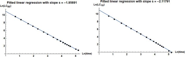
Linear regression of the natural logarithm (Ln) of LC₅₀ (left) and LC₁₀ (right) values vs. the natural logarithm of the associated exposure time (using equation 2), based on data from Jachimowicz and El Sherbiny (1975). According to the LC₅₀ (left), the slope value of the linear regression, which quantifies Haber's exponent, is −1.95691 with 95% confidence interval [−1.97486, −1.93896]. Also, the intercept parameter (log k) is 10.9746 with 95% confidence interval [10.9104, 11.0389]. According to the LC₁₀ (right), s = −2.11791 with 95% confidence interval [−2.14663, −2.08919], and log k = 11.0802 with 95% confidence interval [10.9775, 11.183]

• LC₁₀: lethal concentration 10%, LC₅₀: lethal concentration 10%; Ln: natural logarithm.

In line with the BMD analysis described earlier (see Section 3.1.6.1), effective concentrations (LC₅₀ and LC₁₀) clearly differ across the two data sets. However, BMC is somewhat more conservative than the LC₁₀ at 20 days from the TRT analyses; i.e. the upper bound of the BMC (Table 3) is lower than the LC₁₀ point estimate at 20 days (Table 4). This is probably caused by differences in methodology, e.g. BMCLs/BMDLs are based on modelling of data at specific times points while TRT modelling uses the full survival data as a basis. Also, a model averaging approach is used within the descriptive BMD analysis while the TRT assessment uses a toxicokinetic–toxicodynamic modelling framework (GUTS) and applies a specific dose‐response model (log‐logistic) on top of predictions from the GUTS model.

In principle, the methodology followed in the TRT analysis allows for estimation of the concentration‐response relation and LC values at every time point. However, data on bee lifespan were considered in order to select meaningful times for the assessment. According to a recent review on bee background mortality (EFSA, 2020), the 95th percentile lifespan of a worker honey bee during the active period is 45.4 days. ⁸ In order to use a conservative estimate, a reference time of 50 days was therefore used as one reference time. Similarly, the same review provides data on the survival of bees in winter. Most data (all but one study) showed that the wintering period lasted less than 180 days; hence, this was taken as another reference time. Additionally, an intermediate reference time was arbitrarily set at 90 days.

According to the TRT assessment, LC₁₀ values from the two studies at 50, 90 and 180 days are estimated to be a factor 7.3–7.9, 18–22 and 73–160 lower compared to the LC₁₀ associated with 20 days of exposure. For the LC₅₀, the corresponding factors are 5.5–5.7, 13–17, and 51–60, respectively, indicating a less pronounced effect considering this LC that appears to become of practical significance at higher time points e.g. 180 days. Using the latter factors for dose adjustment (i.e. the LC₅₀ ratios are regarded to be more stable), the BMDL range across studies at 20 days of exposure (1.16–18 µg/bee per day) may be extrapolated to 0.21–3.1, 0.091–1.1 and 0.019–0.35 µg/bee per day for time points of 50, 90 and 180 days, respectively.

3.2. Occurrence data

3.2.1. Occurrence data submitted to EFSA

3.2.1.1. Data set A – Data submitted by EU Member States

By June 2021, in total, 22 analytical results on HMF in bee feed were available in the EFSA database from the year 2019 from Belgium. In addition, data providers from Slovenia and Germany indicated the availability of occurrence data on HMF in bee feed and upon request by EFSA have submitted these data through the data collection framework of EFSA in August 2021. Thus, in total, 219 analytical results were made available from three MS. (Data set A).

One entry was excluded because the moisture percentage was unrealistically low and it was not possible to identify the type of product, or if it is further diluted when given for bees. The remaining 218 samples were collected between 2013 and 2020 by Belgium, Slovenia and Germany from different types of bee feed.

Most of the samples (99%) were analysed by HPLC with standard detection methods (with range of LODs of 1–2 mg/kg and LOQs of 1–10 mg/kg), while two samples were analysed by spectrometry. For 78 samples, information on the LOQ or LOD were not available. The raw data are presented in Annex B, Table 1. From the 218 samples, 167 (77%) were quantified values. Regarding the sampling strategies (as described and defined in EFSA, 2013a,b), one sample was taken by suspect sampling, while others by objective sampling (44%) or selective sampling (10%), or the sampling strategy was not specified (45%). Samples were taken at different locations: on the farm (n = 47) or at the manufacturer (n = 27), at the distribution (wholesale or retail) points (n = 47), one sample at the packing centre, and in 96 cases, the sampling point was not specified.

It was noted that five samples for complementary feed originated from Serbia and Bosnia‐Herzegovina provided by Slovenia and collected in 2013, had unusually high occurrence levels (more than an order of magnitude higher than all other samples), namely 870, 690, 640, 370 and 360 mg/kg.

In order to summarise the occurrence data received, feed data were regrouped into four different categories:

• Complementary feed (includes: complementary feed [incomplete diet], unspecified complementary feed),

• Complete feed (includes: feed [not specified], compound feed, complete feed),

• Sugar syrup (includes: beet sugar[sucrose] feed, glucose syrup, sugar syrup),

• Apiculture by‐products (bee bread, based on the provider’s information).

In terms of application, sugar and moisture content, no major differences were found between sugar syrup, complementary‐ and complete feed; moreover, it was not always clear if the choices of the categories by the data providers are consistent; thus, the total occurrence level for all samples was also calculated. Bee bread was not taken into account in the assessment.

The different types of feeds analysed, and summary statistics of occurrence levels are presented in Table 5.

Table 5.

Overview on occurrence data received from EU Member States

Feed type	n samples	Left‐censored (%)	Mean LB (mg/kg)	Mean UB (mg/kg)	P95 LB(a) (mg/kg)	P95 UB(a) (mg/kg)
Complementary feed(b)	95	36%	38.5	39.1	360	360
Complete feed(c)	31	6%	15.1	15.2	–	–
Sugar syrup(d)	90	17%	17.4	17.7	36.4	36.4
Bee bread (not used)	2	0%	5.9	5.9	–	–
Total  (without bee bread)	216	24%	26.4	26.7	42.0	42.0

LB: lower bound; UB: upper bound; n: number; P95: 95th percentile.

^aThe 95th percentile estimates obtained on categories with less than 60 observations may not be statistically robust (EFSA, 2011). Those values were not included in this table.

^b Complementary feed means compound feed which has a high content of certain substances, and due to its composition suffices for the daily ration of a honey bee only if used together with another feed.

^cComplete feed is compound feed that has a composition sufficient for the daily ration of a honey bee. The provider of these data noted that the data designated as complete feed might also be complementary feed.

^dSugar syrup contains of 72.2% dry matter.

No further information was available regarding when the sampled feeds were produced, and under which conditions (e.g. temperature) the feeds were stored between the production and the sampling or analysis date.

3.2.1.2. Data set B – Data submitted by industry

In addition to the data extracted from the EFSA data warehouse of another data set containing summary statistics of 88 analytical results on HMF in a ready‐to‐use, liquid sugar‐based product used for late winter feeding of bees, were submitted by a European company. The samples were analysed by HPLC‐RP‐DAD with an LOQ of 1 mg/kg after a maximum 36 months of storage at 20°C and 30°C. It was found that initial concentration levels increased with time especially at a higher temperature up to a mean of 146 mg/kg (wet weight). The data submitted by Industry at a are summarised in Table 6.

Table 6.

Overview of analytical data received from industry

Temperature	Storage period (month)	n = 57	Mean (mg/kg, ww)	Temperature	Storage period (month)	n = 31	Mean (mg/kg, ww)
20°C	0	5	21.5	30°C	0	3	23.3
	3	5	23.7		3	3	30.9
	6	5	24.5		6	3	37.8
	9	5	26.7		9	3	46.8
	12	5	27.6		12	3	58.7
	15	4	33.1		15	2	63.1
	18	4	30.6		18	2	71.1
	21	4	33.1		21	2	85.1
	24	4	35.5		24	2	97.9
	27	4	37.9		27	2	112.7
	30	4	39.5		30	2	123.1
	33	4	41.9		33	2	133.0
	36	4	39.5		36	2	146.2

n: number; ww: wet weight.

HMF content was measured in total of 57 samples of an industry product stored in intervals of 3 months at storage temperatures of 20°C and 30°C (see Annex Table 7) for 36 months. These data show that HMF levels increased in the industry product over time. While at a temperature of 20°C, these changes were minimal within the first 9 months of storage, they were already pronounced at 30°C.

3.2.2. Occurrence data from public literature

Occurrence of HMF in bee feed has been reported in public literature, where different commonly used commercial products as well as home‐made bee feeds have been examined. As already mentioned in previous sections, bee feeds containing water (syrups) or prepared with water (fondants and candies) are likely to contain HMF, particularly if the fructose content is high and the feed has been prepared at elevated temperatures or stored for prolonged times. For example, Ruiz‐Matute et al. (2010) reported HMF levels ranging from 10 to 60 mg/kg of syrup have been found in HFCS from a bee supply house. Higher HMF amounts of up to 130 mg/kg syrup were analysed for feeds and stored over 12 months in metal tanks exposed to sunlight.

Syrups from the same producers were analysed by LeBlanc et al. (2009). HMF concentrations in freshly made syrups ranged between 3.1 and 28.7 mg/kg. Over a period of 36 days, HMF concentrations were stable at 30°C but increased to 15–70 mg/kg at 40°C, 50–250 mg/kg at 50°C and drastically up to 20,000–35,000 mg/kg at 70°C in some samples.

Frizzera et al. (2020) investigated home‐made sucrose syrups with pH and temperature as variables. Freshly made syrups using 25°C, 50°C and 110°C with pH values of 7 for the untreated mixture and 2 after addition of lemon juice were tested for HMF levels. The authors found HMF values as low as 2–4 mg/kg for syrups without lemon juice at all temperatures and levels up to 95 mg/kg when acidity and high temperature were combined during their preparation.

Summarising, HMF concentrations in bee feed reported in the public literature varied widely depending on production methods (from 3.1 to 35,000 mg/kg feed) and were only available in summarised form and were therefore not used for the development of exposure scenarios.

3.2.3. Occurrence data used for the assessment

Exposure assessments have been carried out using separately data sets A and B. Overall, the data received from MSs (data set A) upon the call for data on HMF launched by EFSA, contained 218 analytical results coming from three EU MS and of which 23% were left censored. No information about composition, age or storage temperature of the feed samples was provided with these data. Two results available on bee bread were excluded from the assessment as bee bread is a specific product and the number of samples was insufficient to use them for a reliable exposure assessment.

Thus, 216 samples on complementary‐ and complete feed and sugar syrup were considered for exposure scenarios different scenarios (a) considering mean LB/UB values of these three feed categories in separate scenarios, (b) merging all 216 samples and using their LB/UB mean values and was used to estimate the exposure and excluding exceptionally high values for complementary feed were excluded.

Data set B, the analytical data set with the Industry product (for details, see Section 3.2.1.2) was considered for a separate exposure scenario because information on storage time and temperature was only available for these data. The exposure scenarios using the data from Industry (Data set B, where HMF concentrations were analysed upon different storage times) were developed using HMF concentrations upon storage of bee feed at 20°C for either 3, 6, 9 or 12 months as this temperature reflects the recommended storage temperatures and realistic temperatures during the feeding period in the bee hive, and the storage times reflect the maximum shelf‐life recommended by bee feed producers (usually 12–18 months for syrups).

3.3. Feed consumption data

In the absence of measured consumption data, a feed intake of 8.8 mg sugar per day for winter thermoregulation (EFSA, 2012) as described in Section 3.3 was considered as the most appropriate intake value in the cold season where bee feed is usually given. For larvae, a sugar consumption of 9.3 mg per day was used for exposure assessment (Krainer et al., 2016).

To calculate the feed intakes for the exposure calculations, a 72% of dry matter content was used, as this is the usual dry matter content of a sugar syrup.

3.4. Exposure assessment

Exposure assessments for worker bees (winter bees) have been carried out with the HMF levels reported in data sets A and B assuming exclusive consumption of bee feed and a default consumption of 8.8 mg sugar per day for worker bees. Likewise, exposure assessments for larvae have been carried out using a consumption value of 9.3 mg sugar per day per larvae which has been derived from the consumption values reported in the study from Krainer et al. (2016) and the HMF values reported in data sets A and B. It has to be noted here that the assessment for larvae assumes direct uptake of HMF in bee feed as is the case in a laboratory study, while in a field setting larvae are fed by nursing bees. In the colony, nurse bees take up pollen and nectar and use their pharyngeal glands to produce processed food. It has been shown previously that xenobiotics concentrations (i.e. pesticides) are reduced in feed for larvae via this process (Johnson and Percel, 2013; Böhme et al., 2018). Thus, actual exposures are likely lower; however, there is insufficient data to quantify this, and thus, the exposure calculations are used as they are, albeit knowing that they are likely conservative.

Table 7 provides an overview about the exposure scenarios and estimates for worker bees and larvae.

Table 7.

Overview about exposure assessment scenarios and results for worker bees and larvae

	Feed type		n of samples	Storage temperature of feed (°C)	Average concentration (mg/kg ww) (LB/UB)	P95 concentration (mg/kg ww) (LB/UB)(a)	Exposure worker bees (μg per day, LB/UB) with mean concentration	Exposure worker bees (μg per day, LB/UB) with P95 concentration	Exposure larvae (μg per day, LB/UB) with mean concentration	Exposure larvae (μg per day, LB/UB) with P95 concentration
Data set A	Complementary feed		95	n.a.	38.5/39.1	360/360	0.47/0.48	4.40/4.40	0.50/0.51	4.65/4.65
	Complementary feed (without outliers)		90	n.a.	8.1/8.7	25/25	0.10/0.11	0.31/0.31	0.10/0.11	0.32/0.32
	Complete feed		31	n.a.	15.1/15.2	‐‐	0.18/0.19	‐‐	0.20/0.20	‐‐
	Sugar syrup		90	n.a.	17.4/17.7	36.4/36.4	0.21/0.22	0.44/0.44	0.22/0.23	0.47/0.47
	Complementary feed, complete feed, sugar syrup		216	n.a.	26.4/26.7	42.0/42.0	0.32/0.33	0.51/0.51	0.34/0.34	0.54/0.54
	Complementary, complete feed, sugar syrup (without outliers)		211	n.a.	13.1/13.5	35.0/35.0	0.16/0.17	0.43/0.43	0.17/0.17	0.45/0.45
Data set B	Winter bee feed stored	3 months	5	20	23.7	‐‐	0.29(b)	‐‐	0.31	‐‐
		6 months	5	20	24.5	‐‐	0.3	‐‐	0.32	‐‐
		9 months	5	20	26.7	‐‐	0.33	‐‐	0.35	‐‐
		12 months	5	20	27.6	‐‐	0.34	‐‐	0.36	‐‐

LB: lower bound; n: number; n.a.: not available; UB: upper bound; ww: wet weight; To calculate the feed intakes a 72% of dry matter content was used, as it is the usual dry matter content of a sugar syrup.

^aThe 95th percentile estimates obtained on categories with less than 60 observations may not be statistically robust (EFSA, 2011). Those values were not included in this table.

^bFor Data set B, LB and UB calculations were the same as all samples were quantified.

For worker bees, using average HMF concentrations from Data set A resulted in the highest exposure estimates at LB/UB, respectively, of 0.47/0.48 μg/bee per day for complementary feed (n = 95). They were much lower (0.1/0.11 μg/bee per day) when excluding the exceptionally high levels (n = 5) contained in these data subset. Exposures amounted to 0.18/0.19 and 0.21/0.22 μg/bee per day using the subsets ‘complete feed’ (n = 31) and ‘sugar syrup’ (n = 90), respectively.

When combining the data on complementary feed, complete feed and sugar syrup (including the extreme levels on complementary feed) resulting in a more comprehensive data set (n = 216), an exposure of 0.32/0.33 μg/bee per day was estimated. Without the outliers (n = 211) 0.16/0.17 μg/bee per day exposure was found.

A brand loyalty exposure scenario using the P95 concentrations from Data set A was also calculated to reflect possible and likely inappropriate production/storage condition practices of feeding worker bees with only one product during the feeding period. This scenario that includes the exceptionally high values observed in five complementary feed samples which are about an order of magnitude higher than those usually observed in bee feed, results in an P95 exposure for worker bees up to 4.40 μg/bee per day.

Using Data set B, exposures depending on storage time of bee feed varied between 0.29 and 0.34 μg/bee per day depending on storage time.

In order to be able to calculate exposure estimates also for larvae, it was assumed that their feed contains the same amount of HMF as the bee feed given to workers. This is likely an overestimation as larvae are fed via the nurses and thus are exposed to much lower levels of HMF (see this Section, above), albeit, this cannot be quantified.

For larvae, corresponding exposure estimates at LB/UB were 0.50/0.51 μg/larvae per day for complementary feed and 0.10/0.11 μg/larvae per day when excluding the exceptionally high levels in the data subset. Exposures amounted to 0.20 and 0.22/0.23 μg/larvae per day using the subsets ‘complete feed’ and ‘sugar syrup’, respectively.

When considering a similar brand loyalty exposure scenario than it was done for feeding worker bees, it results in an P95 exposure for larvae up to 4.65 μg/larva per day.

When combining the data on complementary feed, complete feed and sugar syrup (including the extreme levels from the subset on complementary feed), an exposure of 0.34 μg/larvae per day resulted.

Using Data set B, exposures depending on storage time of bee feed ranged between 0.31 and 0.36 μg/larvae per day.

3.5. Risk characterisation

3.5.1. Risk characterisation using BMD calculations as reference point

A BMDL₁₀ of 1.16 μg/bee per day is used as the primary Reference Point for bee toxicity, representing the lower end of the BMDL interval (1.16–18 μg/bee per day) across critical studies. This reference point is used for risk characterisation related to worker bees, also applicable for larvae.

The range of exposure scenarios, based on mean occurrence levels, across data set A and B in Table 7 for worker bees, i.e. 0.1–0.48 μg/bee per day, are all below the Reference Point. More specifically, there is a margin of exposure in the range of 2.4–12. The exposure scenario with the highest number of samples (n = 216, 0.32/0.33 μg/bee per day) is a factor 3.5 below the reference point. Considering the mortality rates that would trigger a concern for bee health as laid down in the protection goals for honey bees (see Section 3.1.5) the CONTAM Panel did not identify a concern for the health of worker bees due to exposure to HMF via bee feed.

For larvae, all exposure scenarios, based on mean occurrence levels (0.1–0.51 μg/larva per day), are also below the RP. Margin of exposures in the range of 2.3–12 are observed, and the exposure scenario with the highest number of samples (0.34 μg/larva per day) is a factor 3.4 below the RP. Therefore, based on the same considerations as for honey bees described above also no concern for the health of larvae is apparent, especially since larvae are not directly exposed to bee feed but only via the nurses, and thus actual exposures of larvae to HMF are likely to be much lower.

Upper 95th percentiles of exposure, across scenarios in Table 7, are also below the RP. The exception is the complementary feed group according a brand loyalty scenario approach where the highest P95 exposure both for worker bees and larvae could exceed the RP. As noted earlier, the extreme occurrence levels are likely to be the result of inappropriate production/storage conditions practices.

No data on toxicity or exposure for the queen and drones are available, but it can be assumed that the assessment for worker bees is sufficiently conservative to also cover these bees. It is unlikely that drones are exposed to HMF via bee feed as they are fed by nurses and are not present in the beehive in the cold season. Queens are fed only with royal jelly secreted from glands of worker bees, and thus, exposure to HMF via bee feed is likely much lower than that of worker bees who feed directly on bee feed.

3.5.2. Risk characterisation accounting for time‐reinforced toxicity

Since results indicated that HMF has a clear TRT behaviour (Section 3.1.6.1) an extended risk characterisation was performed, which is of particular relevance for winter bees. Based on the assessment of TRT, reference point intervals of 0.21–3.1, 0.091–1.1 and 0.019–0.35 µg/bee per day were derived for exposure durations of 50, 90 and 180 days, respectively. The intervals reflect uncertainty depending on critical study.

The range of exposure scenarios for adult bees, based on mean occurrence levels (i.e. 0.1–0.48 μg/bee per day), is not fully below any of the three reference point intervals. The exposure scenario with the highest number of samples (0.32/0.33 μg/bee per day), which also reflects the most typical scenario in Table 7, is in the lower end of the reference point interval for an exposure duration of 50 and 90 days. Considering an exposure duration of 180 days, this exposure scenario is, however, located in the upper end of the reference point interval. Therefore, the CONTAM panel identifies a potential concern for the health of winter bees exposed for several months.

The considerations made above for each of the extended exposure durations (50, 90, 180 days) also apply well across exposure scenarios in Table 7, including 95th percentiles of exposure except for the complementary feed group due to a few extreme occurrence values, as the consequence of likely inappropriate storage conditions practices is not regarded appropriate for guiding the risk characterisation at European level.

Due to a narrow or no margin of exposures when accounting for TRT, assessment of uncertainty is regarded to become of higher practical importance motivating the consideration of reference point intervals rather than the lowest value. The potential concern associated with prolonged exposures is further addressed as part of the uncertainty analysis.

3.6. Back calculations

Considering the parameters used in the first exposure scenario (workers bees consuming 8.8 mg sugar per day), a calculated daily concentration of 96 mg HMF/kg bee feed would lead to a daily exposure of 1.16 μg HMF per day (the primary reference point for bee health) and thus still not be of obvious concern for bee health. For larvae, consuming 9.3 mg sugar per day, a concentration of 91 HMF/kg bee feed would lead to a daily exposure of 1.16 μg HMF per day and thus still not be of obvious concern for larvae.

3.6.1. Back calculations accounting for TRT

Using the bee uptake for adult/worker bees (8.8 mg sugar per day), back calculations were also performed using the adjusted reference point intervals that were derived on the basis of results from the TRT assessment. Concentrations of 131, 49 and 15 mg HMF/kg bee feed were calculated corresponding to daily exposures of 1.59, 0.59 and 0.18 μg HMF, respectively, at feeding days 50, 90 and 180. These daily exposures are centrally located (corresponding to the arithmetic average) within adjusted reference point intervals at 50, 90 and 180 days, respectively, placing equal weight on the two critical studies.

3.7. Uncertainty analysis

The evaluation of uncertainty in the present assessment was performed following the principles laid down in the guidance on uncertainty analysis in scientific assessments (EFSA Scientific Committee, 2018), considering also the specific nature of this Opinion. This includes to present information of the sources of uncertainties identified, and their overall impact on the risk assessment.

To harmonise uncertainty analyses, the CONTAM panel has developed a road map that structures the risk assessment process in broader groupings, as well as subgroupings. Sets of questions have also been defined to help the collection of uncertainties. Table 8 describes the part of the road map that is of relevance for this Opinion, which excludes aspects related to human health risk assessment including those related to human exposure assessment methodology. There are four overarching elements of the road map: (i) chemical characterisation and analytical methods, (ii) exposure assessment, (iii) hazard identification and characterisation and (iv) risk characterisation. Uncertainties identified within each of these categories are summarised in Table 8 and described in more detail in subsections below.

Table 8.

Elements of the CONTAM road map regarded to be of potential relevance for the uncertainty analysis

Main group	Subgroup	Questions help collection of uncertainties	Identified uncertainties in the risk assessment of HMF
Chemical characterisation and analytical methods	Chemical characterisation	Is there uncertainty associated with the dose? This may relate to losses due to evaporation, the presence of impurities or the exact composition of the material	No specific uncertainties were identified
	Analytical methods	Is there uncertainty due to the validation of the analytical method? This may include identification, sensitivity and recovery.	No specific uncertainties were identified
Exposure assessment	Occurrence data: Data reporting and representativeness	Is there uncertainty on whether there are missing information or errors in the reported occurrence data?	Data set A: – Uncertainty due to data only available from three MSs – No information about storage time and temperature. – A few outliers were identified – Differences between the application, ingredients and interpretation of different feed types are not fully justified/explained Data set B: – Only few data points within subsets (n = 5) used for the exposure assessment – Data are available from one EU company, for only one specific product
		Is there uncertainty in the occurrence data due to few data?
		Is there uncertainty in the information on processing, e.g. processing prior to the analysis of the samples? This regards sample preparation
		Is there uncertainty due to that the occurrence data maybe not are representative on year, sampling country and origin?
	Consumption data: data reporting and representativeness	Is there uncertainty in the consumption data, e.g. due to use of default value and assumptions (e.g. in EFSA opinion)	Uncertainty in consumption scenario used for workers bees (8.8 mg sugar per day). Uncertainty due to variation in feeds used across critical studies, and since raw data were only partially reported
	Exposure estimates		Uncertainty due to uncertainty in default values used for consumptions scenarios, and uncertainty in occurrence data
Hazard identification and characterisation	ADME	Is there uncertainty in any aspect of ADME? This may include insufficient information on absorption of the parent compound, accumulation potential, metabolism (degradation/hydrolysis/reduction) or transfer rate to animal products.	Uncertainty due to lack of data regarding ADME in bees
	Animal studies – study design	Are there uncertainties in the design of the studies in experimental animals? (including that available studies are limited to certain types of bees)	Uncertainty in extrapolation of results for worker bees to other types of bees within the same and other subspecies
	Animal studies – critical effect		Not regarded relevant. Mortality initially decided to be used as the critical effect
	Genotoxicity	Is there uncertainty on the genotoxicity of the substance (e.g. due to insufficient/inconclusive data or inconsistent results)?	Not regarded relevant. Mortality initially decided to be used as the critical effect
	Mode of action	Are there uncertainties on the MoA of the substance that could affect the conclusions of the risk assessment?	Little is known of the mode of action, but uncertainty of low relevance for risk characterisation
	Interactions	Is there uncertainty on the extent of effects due to co‐exposure or similar (e.g. a potential effect of pH has been discussed)?	Uncertainty due to potential synergism between HMF and unmeasured stressors, or acidity
	Dose–response analysis of critical endpoint(s)	Is there uncertainty regarding the dose response analysis e.g. trend occurrence, large data variation, possible covariants?	Uncertainty in dose‐response analysis due to conversion of concentrations to doses
	Reference point	Are there uncertainties in the selection of the RP that are not covered by the BMD confidence interval e.g. is model uncertainty covered?	Uncertainty due to variation in BMD results across critical studies, and with respect to the selected BMR
		Is there uncertainty on the biological relevance of the selected BMR and (how) will this affect the results from BMD analysis?
Risk characterisation	Uncertainty factors	Is there uncertainty in the selected (default or specific) UFs	Uncertainty in extrapolation factor derived from assessment of time‐reinforced toxicity
	Risk metric		Uncertainty due to uncertainty in exposure estimates, reference point and uncertainty factor

ADME: absorption, distribution, metabolism, excretion; BMD: benchmark dose; HMF: hydroxymethyl furfural; MoA: mode of action; UF: uncertainty factor.

3.7.1. Chemical characterisation and analytical methods

No specific uncertainties were identified related to chemical characterisation. HMF is a solid compound with a melting point of 30–34°C. In the critical studies for the assessment, it was purchased from a supplier and added to the bee feed. Although the purity was not given in these papers, data sheets state that it is > 98%. The chemical structure is established by spectroscopic methods (NMR, MS).

Also, no specific uncertainties were identified related to the analytical method. Pure reference material was available for validating the HPLC and Winkler method.

3.7.2. Hazard identification and characterisation

There are significant uncertainties related to the toxicokinetics of HMF because of the lack of relevant data.

Based on the available data, mortality was identified as the critical endpoint for hazard identification and characterisation. Uncertainty associated with selection of the critical effect was therefore regarded as not relevant for the overall risk characterisation. Likewise, uncertainty related to genotoxicity was not considered relevant for this Opinion, and the uncertainty related to the HMF mode of action (discussed in Section 3.1.3) was considered to be of low relevance.

The three studies considered suitable for derivation of a reference point for bee health (Jachimowicz and El Sherbiny, 1975; Krainer et al., 2016; Gregorc et al., 2020) were conducted with Apis mellifera carnica. There is no evidence that this subspecies is more sensitive to HMF when compared to B honey bee subspecies. However, uncertainties remain regarding the extrapolation to other honey bee subspecies.

The feeds used in the different experiments varied, including e.g. invert sugar solutions or sugar candies. Consumption data were only partially reported. Also, the feed used in the key studies does not comply with OECD guidelines for toxicity testing. The reference point is derived from data observed in worker bees and 20 days of exposure (Jachimowicz and El Sherbiny, 1975). Moreover, as noted in the Section 3.1.6, the results for worker bees are regarded to also cover toxicity in larvae, and while it is assumed that it also covers drones and queens the lack of data prevented quantitative analysis of this issue, which introduces uncertainty.

The exposure period of 20 days covers most of the entire average life span of a summer bee (15–38 days). However, the results of the assessment indicated that HMF has clear TRT characteristics. Thus, the primary reference point for bee health (1.16 µg/bee per day), based on 20 days of exposure, may be not apply for winter bees which can be exposed for much longer. This was accounted for by the derivation of adjusted reference points for extended exposure durations, but there is uncertainty in the extrapolation factors used in this process.

3.7.2.1. Interactions

Although the control bees have been exposed to the same conditions as the treated bees, in the suitable toxicity studies, potential synergism between HMF and unmeasured stressors cannot be excluded (e.g. viruses, Nosema infection). In addition, it has been demonstrated that low pH (pH = 2.8) in the syrup reduces bee survival (Frizzera et al., 2020). Even though Jachimowicz and El Sherbiny (1975) did not find an effect of acidity (pH of 3.9 in control and test feed) on the mortality rate, a synergistic interaction between acidity and the presence of HMF cannot be excluded.

3.7.2.2. Dose‐response analysis of critical endpoint, and derivation of reference point

Information on feed consumption of worker bees was lacking in the three suitable studies. For conversion of concentrations to doses in laboratory studies, a value of 13.5 mg/sugar per bee per day, as reported in the literature was used. This introduces some uncertainty in the derivation of the BMDs. For larvae, using data from the literature, a density of sugar solutions equal to 1 was assumed as a pragmatic approach to convert consumption information on a volume basis to weight basis in the process dose calculations, which introduces additional uncertainty in this case.

BMC/BMD results for one of the suitable studies (Krainer et al., 2016) were associated with extrapolation. As noted in the section on derivation of reference point (Section 3.1.6), this implied that the highest BMDL across suitable studies was not regarded to be reliable, and it was therefore excluded from further consideration. Even so, a discrepancy in BMDLs between the two other suitable studies (Jachimowicz and El Sherbiny, 1975; Gregorc et al., 2020) remains (BMDL₁₀ range is 1.16–18 µg/bee per day), which describes introduces uncertainty in the reference point (BMDL₁₀).

While there is uncertainty related to what would constitute an appropriate BMR for bee mortality, this is not regarded to have a practical impact relative to the BMDL difference across studies discussed above. The default BMR of 0.1 used is also supported by the protection goals for honey bees that considers a maximum reduction in colony size of 10% as a threshold for concern, agreed by the EU agricultural ministers (Council of the EU, 2021).

3.7.3. Exposure assessment

Two occurrence data sets were available. Data set A from EU MS and data set B from Industry. Data set A contained of 219 analytical samples used for the assessment from three EU MS and the representativeness for the entire EU is thus limited and therefore constitutes an important uncertainty. Furthermore, there was no information available on the age of the samples when tested and the temperature of storage which are important factors for HMF contents which represents an uncertainty. The data set contained five very high occurrence values sampled in 2013, which can be considered as outliers. However, as the samples were taken at the distribution point (retail or wholesale), a brand loyal exposure scenario considering their presence on the market was also calculated.

For data set B, that contained a total of 88 analytical results, both storage time and temperature were available for a single bee feed product. Only a fraction of the data was used which was considered representative for the usual storage and feeding conditions, and the subsets for the different scenarios were small (n = 5). Considering the low number of samples, and that the data were only collected on one single bee feed product, it constitutes some uncertainty. However, as bee feeds based on sugar syrups has similar sugar content, and the recommended storage conditions are defined by the producer of the feed, the assessment most probably represents similar products of other brands as well.

No consumption data was available for worker bees and larvae. Therefore, default values had to be applied for worker bees (8.8 mg sugar per day) and for larvae consumption reported in a single study was used (9.3 mg sugar per day) where feed was given in a pipette while larvae are fed via nurses for exposure assessment. This introduces uncertainty. Also, there is uncertainty regarding the consumption within the critical studies for this assessment, which affect the conversion of concentrations to doses as part of the dose–response analysis (see above). The assumption that the exposure assessments also apply for drones and queens is likely an overestimation.

The combined effect of uncertainties described above related to the consumption and concentration data will be of importance for the exposure assessment/metrics.

3.7.4. Risk characterisation

It was regarded not appropriate to use an uncertainty factor for interspecies differences since the species tested was also the species of concern. The results from assessment of TRT, however, are represented in the format of uncertainty/adjustment factors. As noted earlier, there is uncertainty in the factors used for derivation of adjusted reference points for extended exposure durations. However, quantified TRT characteristic for the two most critical studies are similar, with slope factors close to –2 (and narrow confidence intervals, relatively speaking) in spite of the systematic difference in BMD results across the same studies. While the outcome from the TRT assessment was rather consistent across data set, the overall result from this type of exercise may, however, be affected by broader issues described below, which adds to the uncertainty.

The TRT analysis attempts to estimate the effect on worker honey bees following a long exposure period to HMF during winter time. However, the entire hazard assessment is based on laboratory tests performed on spring/summer bees, i.e. during their active period. The use of cages limits very much the energy expenditure compared to free‐flying bees and possibly also compared to nurses. Nevertheless, the metabolism of the tested organisms is still the one of active bees, which might not be comparable with the one of a winter bee. As a matter of fact, honey bees undergo a reduction in metabolism during winter, which allows them to save energy and considerably increase their lifespan. This mismatch is an important source of uncertainty. Furthermore, the lack of information on the toxicokinetics and toxicodynamics of HMF in bees makes the effect of different metabolism rates on the bee sensitivity/tolerance towards HMF rather unpredictable. The TRT analysis may indicate slow kinetics already in active bees, but further information would be needed before attempting a meaningful prediction.

The combined effect of uncertainties described above related to the exposure assessment/estimate, reference point and uncertainty factor (TRT assessment) will be of importance at the level of the risk characterisation as well as for the back calculations presented in Section 3.6.

3.7.5. Summary and quantification of the most important uncertainties

From consideration of identified uncertainties (summarised in Table 8), it is regarded that the difference in BMDL values between critical studies is the factor that individually has the largest impact on the risk characterisation. Also, while the estimated time‐reinforcement factor was consistent between studies broader issues, discussed in previous section, that are not easily quantified may affect the assessment of TRT.

Monte Carlo simulations were conducted to support the quantification of overall uncertainty, where uncertainties in parameters were characterised by probability distributions. Besides the discrepancy between BMDL results across studies, this analysis accounts for uncertainty in the model for time‐dependent toxicity, by utilising uncertainty distributions derived from the 95% confidence intervals estimated from the linear regression and judgements on uncertainty in the models. Also, the consecutive derivation of adjustment factors and adjusted reference point intervals is taken into account. On top of this, results across all exposure scenarios in Table 7 are considered within the simulations as part of an extended risk characterisation. Results in Table 9 describe the probability that the exposure, under defined cases (Case 1–3), exceeds simulated reference points. Details behind the approach used are given in association with Table 9.

Table 9.

Uncertainty in simulated reference points, the probability of exceeding them for different exposure durations and associated probability terms

Time point (days)	P95:P05 ratio for simulated reference points(a)	Probability of exceeding simulated reference points under exposure Case 1, 2, and 3(b)
		Case 1(c): Simulated exposure	Case 2(d): 0.32 μg per day	Case 3(e): 0.47 μg per day	Probability terms covering Case 1–3(f)
20	Study A: 1.2 (4.1) Study B: 1.3 (14)	0 (< 0.0005)	0 (< 0.0005)	0 (< 0.001)	Almost impossible (0–1%)
50	Study A: 1.2 (5.0) Study B: 1.3 (19)	0.02 (0.06)	0.04 (0.08)	0.09 (0.16)	Extremely unlikely (1–5%) to unlikely (10–33%)
90	Study A: 1.2 (5.7) Study B: 1.4 (24)	0.19 (0.27)	0.26 (0.36)	0.42 (0.48)	Unlikely (10–33%) to about as likely as not (33–66%)
180	Study A: 1.2 (6.7) Study B: 1.4 (33)	0.74 (0.62)	0.99 (0.72)	1.0 (0.79)	About as likely as not (33–66%) to almost certain (99–100%)

Note: The error in estimated parameters of the linear regression of time‐dependent toxicity was assumed to be normally distributed with a standard deviation matched to the 95% confidence intervals for the slope (log s) and intercept (log k) given in Figures 5, 6 and 5, 6 (result associated with the ED₅₀ was used). Considering each of the two studies used for BMDL derivation separately, N = 100,000 values for log s and log k were randomly generated independently from each uncertainty distribution providing N alternative linear models. Using a time point of 20 days as the reference, adjustment factors (AFs) for extrapolation to specified time points were derived for each simulated linear model as the ratio R_T = AF₂₀/AF_T, where T is 20, 50, 90 or 180 days. Adjusted reference points were then derived by dividing the BMDL at 20 days [(i.e. 1.2 μg/bee per day for Jachimowicz and El Sherbiny (1975), and 18 μg/bee per day for Gregorc et al. (2020)] with R_T. For each time point, this exercise provides N alternative reference point intervals, each describing an uncertainty range depending on study.

^aRatio between the upper 95th and lower 5th percentile of simulated reference points (N = 100,000) based on data from Jachimowicz and El Sherbiny (1975) [Study A], and data from Gregorc et al. (2020) [Study B]. Values within parenthesis describe results under an alternative scenario where the standard deviation for log s and log k used in the simulations has been increased by a factor 10.

^bAssuming a uniform distribution, a single value was randomly generated from each of the N = 100,000 reference point intervals (describing study difference), for a given time point. The resulting N simulated reference point values (for a given time point) were then compared to an exposure value according to Case 1, 2 or 3, and probabilities given in the Table correspond to the fraction of exposures that exceeded simulated reference points. Values within parenthesis describe an alternative scenario where the standard deviation for log s and log k has been increased by a factor 10. This implies that the absolute difference between the upper and lower bounds of the 95% confidence intervals in Figures 5, 6 and 5, 6 would also increase by a factor 10. Simulations were performed in Matlab.

^cN exposure values were generated by random sampling (with replacement) of estimated exposures, based on mean occurrence levels, across all scenarios for adult bees in Table 7 (i.e. values of 0.47, 0.10, 0.18, 0.21, 0.32, 0.16 or 0.3 μg per day were used), and compared to the N simulated reference point values for a given time point.

^dA specific exposure of 0.32 μg per day was used, which corresponds to the estimate for adult bees in Table 7, associated with mean occurrence levels, that is based on the highest number of samples.

^eA specific exposure of 0.47 μg per day was used, which is the highest estimate associated with mean occurrence levels for adult bees in Table 7.

^fRelevant probability terms according to the approximate probability scale recommended for harmonised use in EFSA (EFSA Scientific Committee, 2018).

The quantitative information of uncertainty noted above, i.e. 95% confidence intervals, only covers the last step of the TRT approach, i.e. the linear regression of estimated LC values for associated time points. Ideally, the uncertainty across all steps of the approach should be accounted for in a sequential manner: i.e. uncertainty associated with calibration of the TKTD model, fitting of the (log logistic) dose‐response model and the linear regression. Due to time constraints, a more complete quantification of uncertainty along these lines could not be performed. Intuitively, however, if uncertainty is accounted for across all steps within the approach used for TRT assessment, this may increase the uncertainty associated with the model for time‐dependent toxicity in the last step. If so, this would correspond to an increase in the width of a 95% confidence intervals for the slope (log s) and intercept (log k) used as basis for the simulations. It is unclear how large this effect would be but as a pragmatic approach, the standard deviation for log s and log k was increased by a factor 10. Results associated with this additional scenario is also given in Table 9, including the effect at the level of simulated reference points. The overall quantification of uncertainty is based on results in Table 9, and the approximate probability scale recommended for harmonised use in EFSA (EFSA Scientific Committee, 2018) was used for describing the probabilities (i.e. probability terms). Based on the two studies considered, it is regarded almost impossible (probability < 1%, Table 9) that the exposure exceeds the reference point for 20 days of exposure. For an exposure duration of 50 days, it is regarded extremely unlikely to unlikely (probability in the range of 2–16%, Table 9) that the adjusted reference point is exceeded. For 90 days of exposure, it is regarded unlikely, to about as likely as not (probability of about 20–50%) that the adjusted reference point is exceeded. And, for an exposure duration of 180 days, it considered about as likely as not, to almost certain (probability about 60–100%, Table 9) that the adjusted reference point is exceeded. While exposures associated with Case 1 through 3 in Table 9 are based on mean occurrence levels, they also approximately cover upper 95th percentiles of exposures for all feed groups in Table 7 for adults bees (0.31–0.51 μg per day) except ‘complementary feed’ due to a few extreme occurrence values in that data set discussed earlier.

It can be noted that the ratio between the BMDU and BMDL for 20 days is a factor 1.2–1.7 in the original BMD analysis (Table 3). As shown by the ratios between the upper 95th and lower 5th percentiles for simulated reference point in Table 9, the analysis cover this and much higher levels of uncertainty. Modulating the uncertainty in the linear model by a factor of 1 vs. 5 or a factor of 1 vs. 20, instead of a factor of 1 vs. 10, would provide a variation in results that is highly compatible with the probability statements in the last column of Table 9, if not fully identical (data not shown). A further increase in the factor to 30 would describe levels of uncertainty in simulated reference points that are extreme, with P95 to P05 ratios in the range of hundreds to 10s of thousands, and was therefore not considered (data not shown).

4. Conclusions

5‐hydroxymethylfurfural (HMF) is a degradation product of hexoses and is present in honey and various bee feeds. Commercially available bee feeds contain either sucrose or mixtures of glucose and fructose and may contain varying levels of HMF depending on the conditions of production and use. The most important parameters for HMF formation in bee feeds are the type of sugar used, pH, temperature, water activity and concentration of divalent cations of the media. HMF is determined by spectrometric and chromatographic methods.

4.1. Toxicokinetics

• While the toxicokinetics of HMF are well investigated in mammals, no information on the toxicokinetics of HMF in bees could be identified.

4.2. Toxicity

• Several experimental studies have been carried out in which the effect of oral uptake of HMF in bees on mortality/survival was investigated.

• The concentrations of HMF causing mortality in experimental studies varied between 150 and 750 mg/kg bee feed.

• HMF induced mortality significantly aggravates with exposure time.

• Field studies with bees ingesting HMF containing bee feed suggest that feeding with concentrations between 40 and 150 mg HMF/kg bee feed is not detrimental to bee colonies.

4.3. Mode of action

• The mode of action by which HMF induces bee mortality has not been established, but it has been shown that HMF causes histopathological effects in the midgut of bees which were paralleled by increased mortality.

4.4. Identification of critical effects

• Based on the absence of acute toxicity even at high doses, HMF is considered to be of low acute toxicity.

• Increased mortality (decreased survival) rate has been identified as the critical chronic effect of HMF in bees.

4.5. Concentration/dose response assessment

• Three experimental studies have been identified as suitable for assessing the chronic concentration/dose response in worker bees. A benchmark response (BMR) of 10% was identified as appropriate for the critical endpoint. Benchmark doses lower bound with BMR at 10% (BMDL₁₀) of 32.7 μg/bee per day, of 1.16 μg/bee per day and of 18.0 μg/bee per day were calculated from each of the studies.

4.6. Derivation of reference points

• A reference point of 1.16 μg HMF/bee per day was derived based on the lowest BMDL₁₀ seen in the three studies suitable for risk assessment. This was considered as the primary BMDL₁₀ for risk characterisation, even though it was substantially lower than the BMDL₁₀ obtained from the other two studies suitable for risk assessment.

• The reference point of 1.16 μg HMF/bee per day also covers HMF‐induced mortality in larvae, drones and queens for which no or insufficient data are available.

• Since analyses indicated that HMF has clear time reinforced toxicity (TRT) characteristics, additional reference points were established. Based on calculated extrapolations factors, adjusted reference point intervals of 0.21–3.1, 0.091–1.1, 0.019–0.35 µg/bee per day were derived for exposure durations of 50, 90 and 180 days, respectively. The intervals reflect uncertainty depending on critical study.

4.7. Occurrence data

• A total of 219 analytical samples of bee feed from three different EU member states were available and 88 analytical results with bee feed from a European company were available.

4.8. Feed consumption data

• Consumption data for worker bees of bee feed were not available; therefore, the default consumption value of 8.8 mg sugar/bee from EFSA guidance was used for the assessment for worker bees instead. For larvae, a consumption value of 9.3 mg sugar/larvae as reported in the public literature was used for exposure assessments.

4.9. Exposure assessment

• Exposure assessment scenarios for worker bees have been carried out with the HMF levels reported in the data sets from MS and Industry assuming exclusive consumption of bee feed and using consumption values as described above.

• For worker bees, using average HMF concentrations highest exposure estimates at LB/UB, were 0.47/0.48 μg/bee per day for the subset of complementary feed (n = 95) from EU MS. When combining the data on complementary feed, complete feed and sugar syrup (n = 216), an exposure of 0.32/0.33 μg HMF/bee per day resulted. Using the data from industry, exposures depending on storage time of bee feed, varied between 0.29 and 0.34 μg/bee per day.

• For larvae, exposure estimates at LB/UB were 0.50/0.51 μg/larva per day for complementary feed. With the complete data set from EU MS, an exposure of 0.34 μg/larva per day resulted. Using Industry data, exposures, depending on storage time of bee feed ranged between 0.31 and 0.44 μg HMF/larva per day.

• Considering brand loyalty in feeding practises using P95 occurrence values driven by a few exceptionally high occurrence values, which are likely due to inappropriate production/storage of bee feed, provide P95 exposure estimates for worker bees and larvae, respectively, up to 4.40 and 4.65 μg HMF per day.

4.10. Risk characterisation

• The range of mean exposure scenarios for worker bees across data sets A and B in was 0.1–0.48 μg/bee per day, are all below the reference point of 1.16 μg HMF/bee per day. Based on the uncertainty analysis, it is regarded almost impossible (probability < 1%) that the reference point for 20 days of exposure is exceeded. Therefore, for worker bees exposed to HMF via common bee feed, no health concern was identified by the CONTAM Panel.

• For larvae, all mean exposure scenarios (ranging from 0.1 to 0.51 μg/larva per day) are below the RP and margins of exposures in the range of 2.3–12 are observed. Therefore, also no concern for the health of larvae is apparent, even more so since larvae are not directly exposed to bee feed but only via the nurses, and thus, actual exposures of larvae to HMF are likely to be much lower.

• No data on toxicity or exposure for queen and drones are available, but it can be assumed that the assessment for worker bees is sufficiently conservative to also cover these bee casts.

• Accounting for TRT, the range of exposure scenarios for adult bees (i.e. 0.1–0.48 μg/bee per day) is not fully below the reference point intervals established for prolonged exposures. Based on the uncertainty analysis is regarded extremely unlikely to unlikely (probability in the range of 2–16%) that the adjusted reference point for 50 days of exposure is exceeded. It is regarded unlikely, to about as likely as not (probability of about 20–50%) that the adjusted reference point for 90‐day exposure is exceeded. It is considered about as likely as not, to almost certain (probability about 60–100%, Table 9) that the adjusted reference point for 180 days of exposure is exceeded. Therefore, the CONTAM panel identifies a potential concern for the health of bees when they are exposed to HMF via bee feed for several months.

• Using P95 of the occurrence levels for the subset on complementary feed would lead to exposures clearly exceeding the reference points for 20 through 180 days. Considering that the high exposure values are the result of a few samples from a single European country, it is not excluded that inappropriate production/storage conditions were applied. For this reason, the CONTAM Panel defines the high values as exceptional cases and thus not representative for the risk assessment, while suggesting caution in regard of the brand loyalty feeding practices.

4.11. Back calculations

• A concentration of 95 mg HMF/kg bee feed would lead to a calculated daily exposure of 1.16 μg HMF per day and thus still not be of concern for worker bees. For larvae, the corresponding figure is 91 HMF/kg bee feed. In the absence of data, the concentration safe for worker bees also applies for drones and queens.

• Considering adjusted reference point intervals derived on the basis of the TRT assessment concentrations of 131, 49 and 15 mg HMF/kg bee feed were calculated for daily exposures of 1.59, 0.59 and 0.18 μg HMF, respectively, at feeding days 50, 90 and 180 (the daily exposures correspond to the arithmetic averages of adjusted reference point intervals for the three time points).

5. Recommendations

• Further toxicity tests are needed to establish sensitive indicators (e.g. molecular, physiological, behavioural) for adverse effects (acute, chronic and sublethal) induced by exposure to HMF;

• It is recommended to collect consumption data of bee feed in different contexts (e.g. according to various beekeeping settings and environmental conditions) and make them readily accessible (open access) for further analysis;

• It is recommended that a concentration of HMF of no health concern for bees is established in bee feed with appropriate production/storage conditions that is compatible with brand loyalty feeding practices.

• Studies on absorption, distribution (including non‐extractable binding to biomolecules), metabolism and excretion in honey bees including winter bees, preferably using radiolabelled HMF are recommended;

• Investigations on the effect of pH on the toxicity of HMF and HMF containing bee feed are recommended;

• The presence of other toxic constituents in bee feed should be investigated.

Documentation as provided to EFSA

On 29 January 2021, 88 analytical data points on HMF in bee feed were received from a European company.

Abbreviations

AIC

Akaike information criterion

BMC

Benchmark concentration

BMCL₁₀

Benchmark concentration lower bound with BMR at 10%

BMCU₁₀

Benchmark concentration upper bound with BMR at 10%

BMD

Benchmark dose

BMDL₁₀

Benchmark dose lower bound with BMR at 10%

BMDU₁₀

Benchmark dose upper bound with BMR at 10%

BMR

Benchmark reference

CONTAM

Panel on Contaminants in the Food Chain

DAD

diode‐array detector

FDCA

2,5‐furane dicarboxylic acid

GSH

Glutathione

ECHA

European chemical agency

GUTS

General Unified Threshold models of Survival

GUTS‐RED

reduced GUTS

HFCS

high fructose corn syrup

HMFA

5‐hydroxymethyl‐2‐furoic acid

HMFG

5‐hydroxymethyl‐2‐furoyl glycine

HMF

Hydroxymethylfurfural

HPLC‐RP

High performance liquid chromatography – Reverse phase

IHC

International Honey Commission

ISCDDK

in situ cell death detection kit

IT

individual tolerance

LC

Lethal Concentration

LC₅₀

median Lethal Concentration

LDD50

median Lethal Dietary Dose

LOD

Limit of detection

LOQ

Limit of quantification

MLs

maximum levels

NFI‐DTU

National Food Institute ‐ Technical University of Denmark

NOEC

No Observed Effect Concentration

NOEDD

No Observed Effect Dietary Dose

OECD

Organisation for Economic Co‐operation and Development

RASFF

Rapid Alert System for Food and Feed

SD

stochastic death

SMF

5‐sulfoxymethylfurfural

SOPs

standard operational procedures

SSD

Standard Sample Description

TKTD

toxicokinetic‐toxicodynamic

TRT

Time reinforced toxicity

UF

uncertainty factor

UV

Ultraviolet

ww

wet weight

Appendix A – BMD analyses

A.1. BMD analysis of bee mortality (after 20 days) due to the presence of HMF in bee feed (Jachimowicz and El Sherbiny, 1975)

• A) Data description

The endpoint to be analysed is: number of dead bees.

• B) Data used for analysis

HMF in μg/bee per day	Number of dead bees	Total number of bees
0.00	63	500
0.81	75	500
4.05	294	500
20.25	494	500

• C) Selection of the BMR

The benchmark response (BMR) used is an extra risk of 10%. The benchmark dose (BMD) is the dose corresponding to the BMR of interest. A 90% confidence interval for the BMD will be estimated, with lower and upper bound denoted BMDL and BMDU, respectively.

• D) Software used

Results are obtained using the EFSA web‐tool for BMD analysis, which uses the R‐package PROAST, version 70.0, for the underlying calculations.

• E) Results

Response variable: number of dead bees

Fitted models

Model	No.par	loglik	AIC	Accepted	BMDL	BMDU	BMD	conv
null	1	–1,380.81	2,763.62		NA	NA	NA	NA
full	4	–772.00	1,552.00		NA	NA	NA	NA
two.stage	3	–781.15	1,568.30	No	NA	NA	0.663	Yes
log.logist	3	–772.08	1,550.16	Yes	1.35	1.94	1.640	Yes
Weibull	3	–777.75	1,561.50	No	NA	NA	0.850	Yes
log.prob	3	–772.05	1,550.10	Yes	1.19	1.71	1.450	Yes
gamma	3	–775.69	1,557.38	No	NA	NA	0.998	Yes
LVM: Expon. m5‐	4	–772.00	1,552.00	Yes	1.10	2.77	1.640	Yes
LVM: Hill m5‐	4	–772.00	1,552.00	Yes	1.08	2.44	1.590	Yes

Estimated model parameters

two.stage

estimate for a‐ : 0.103

estimate for BMD‐ : 0.663

estimate for c : 0.1344

log.logist

estimate for a‐ : 0.1298

estimate for BMD‐ : 1.64

estimate for c : 2.555

Weibull

estimate for a‐ : 0.1084

estimate for BMD‐ : 0.8503

estimate for c : 1.204

log.prob

estimate for a‐ : 0.1287

estimate for BMD‐ : 1.446

estimate for c : 1.315

gamma

estimate for a‐ : 0.1127

estimate for BMD‐ : 0.998

estimate for c : 1.505

EXP

estimate for a‐ : 1.332

estimate for BMD‐ : 1.637

estimate for c‐ : 0.427

estimate for d‐ : 1.714

estimate for th(fixed) : 0

estimate for sigma(fixed) : 0.25

HILL

estimate for a‐ : 1.332

estimate for BMD‐ : 1.588

estimate for c‐ : 0.3962

estimate for d‐ : 1.839

estimate for sigma(fixed) : 0.25

Weights for model averaging

two.stage	log.logist	Weibull	log.prob	gamma	EXP	HILL
0	0.35	0	0.36	0.01	0.14	0.14

F) Final BMD Values

Subgroup	BMDL	BMDU
All	1.16	1.97

Confidence intervals for the BMD are based on 200 bootstrap data sets.

G) Visualisation

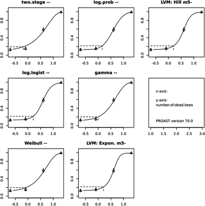
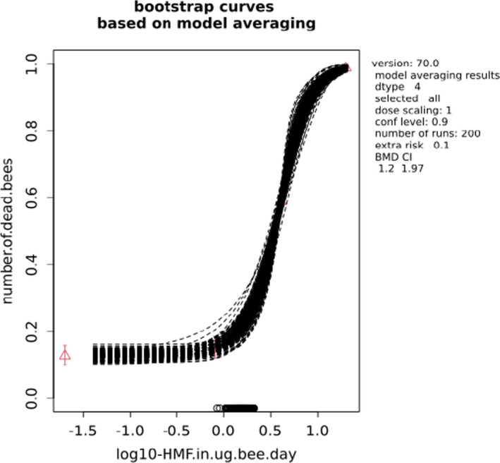
A.2. BMC analysis of bee mortality (after 20 days) due to the presence of HMF in bee feed (Jachimowicz and El Sherbiny, 1975)

A) Data description

The endpoint to be analysed is: number of dead bees.

B) Data used for analysis

HMF in mg/kg feed	Number of dead bees	Total number of bees
0	63	500
30	75	500
150	294	500
750	494	500

C) Selection of the BMR

The benchmark response (BMR) used is an extra risk of 10%. The benchmark concentration (BMC) is the concentration corresponding to the BMR of interest. A 90% confidence interval for the BMC will be estimated, with lower and upper bound denoted BMCL and BMCU, respectively.

D) Software used

Results are obtained using the EFSA web‐tool for BMC analysis, which uses the R‐package PROAST, version 69.0, for the underlying calculations.

E) Results

Response variable: number of dead bees

Fitted models

Model	No.par	loglik	AIC	Accepted	BMCL	BMCU	BMD	conv
Null	1	–1,380.81	2,763.62		NA	NA	NA	NA
Full	4	–772.00	1,552.00		NA	NA	NA	NA
two.stage	3	–781.15	1,568.30	No	NA	NA	24.6	Yes
log.logist	3	–772.08	1,550.16	Yes	50.1	71.7	60.7	Yes
Weibull	3	–777.75	1,561.50	No	NA	NA	31.5	Yes
log.prob	3	–772.05	1,550.10	Yes	44.3	63.5	53.5	Yes
Gamma	3	–775.69	1,557.38	No	NA	NA	37.0	Yes
Logistic	2	–793.82	1,591.64	No	NA	NA	46.1	Yes
Probit	2	–812.95	1,629.90	No	NA	NA	52.1	Yes
LVM: Expon. m5‐	4	–772.00	1,552.00	Yes	40.8	103.0	61.3	Yes
LVM: Hill m5‐	4	–772.00	1,552.00	Yes	40.1	97.0	58.6	Yes

Estimated model parameters

two.stage

estimate for a‐ : 0.103

estimate for BMD‐ : 24.55

estimate for c : 0.1344

log.logist

estimate for a‐ : 0.1298

estimate for BMD‐ : 60.75

estimate for c : 2.555

Weibull

estimate for a‐ : 0.1084

estimate for BMD‐ : 31.49

estimate for c : 1.204

log.prob

estimate for a‐ : 0.1287

estimate for BMD‐ : 53.55

estimate for c : 1.315

gamma

estimate for a‐ : 0.1127

estimate for BMD‐ : 36.96

estimate for c : 1.505

logistic

estimate for a‐ : ‐1.823

estimate for BMD‐ : 46.1

probit

estimate for a‐ : ‐0.9669

estimate for BMD‐ : 52.15

EXP

estimate for a‐ : 1.332

estimate for BMD‐ : 61.33

estimate for c‐ : 0.4271

estimate for d‐ : 1.668

estimate for th(fixed) : 0

estimate for sigma(fixed) : 0.25

HILL

estimate for a‐ : 1.332

estimate for BMD‐ : 58.64

estimate for c‐ : 0.3956

estimate for d‐ : 1.854

estimate for th(fixed) : 0

estimate for sigma(fixed) : 0.25

Weights for model averaging

two.stage	log.logist	Weibull	log.prob	gamma	logistic	probit	EXP	HILL
0	0.35	0	0.36	0.01	0	0	0.14	0.14

F) Final BMC values

Subgroup	BMCL	BMCU
All	42.1	73.7

Confidence intervals for the BMC are based on 200 bootstrap data sets.

G) Visualisation

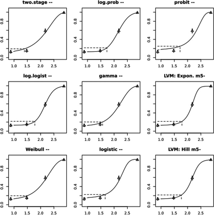
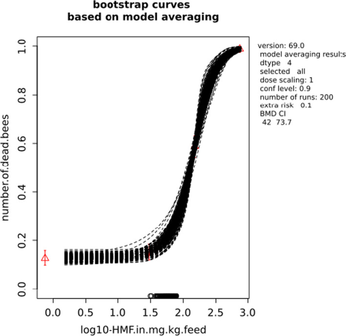
A.3. BMD analysis of bee mortality (after 7 days) due to presence of HMF in bee feed (Krainer et al., 2016 )

A) Data description

The endpoint to be analysed is: number of dead bees.

B) Data used for analysis

HMF in μg/bee per day	Number of dead bees	Total number of bees
0	1	144
54	1	144
108	7	144
216	7	144

C) Selection of the BMR

The benchmark response (BMR) used is an extra risk of 10%. The benchmark dose (BMD) is the dose corresponding to the BMR of interest. A 90% confidence interval for the BMD will be estimated, with lower and upper bound denoted BMDL and BMDU, respectively.

D) Software used

Results are obtained using the EFSA web‐tool for BMD analysis, which uses the R‐package PROAST, version 69.0, for the underlying calculations.

E) Results

Response variable: number of dead bees.

Fitted models

Model	No.par	loglik	AIC	Accepted	BMDL	BMDU	BMD	conv
null	1	–73.11	148.22		NA	NA	NA	NA
full	4	–67.92	143.84		NA	NA	NA	NA
two.stage	3	–69.33	144.66	Yes	274	1,050	443	Yes
log.logist	3	–69.32	144.64	Yes	235	1,760,000	423	Yes
Weibull	3	–69.33	144.66	Yes	235	2,450,000	419	Yes
log.prob	3	–69.24	144.48	Yes	236	903,000	445	Yes
gamma	3	–69.33	144.66	Yes	235	2,150,000	416	Yes
logistic	2	–69.94	143.88	Yes	229	687	305	Yes
probit	2	–69.83	143.66	Yes	230	699	312	Yes
LVM: Expon. m3‐	3	–69.45	144.90	Yes	234	8,410	394	Yes
LVM: Hill m3‐	3	–69.43	144.86	Yes	234	10,800	401	Yes

Estimated model parameters

two.stage

estimate for a‐ : 0.005853

estimate for BMD‐ : 443

estimate for c : 1e‐06

log.logist

estimate for a‐ : 0.005951

estimate for BMD‐ : 423.4

estimate for c : 1.078

Weibull

estimate for a‐ : 0.00596

estimate for BMD‐ : 418.9

estimate for c : 1.058

log.prob

estimate for a‐ : 0.005942

estimate for BMD‐ : 445.2

estimate for c : 0.4779

gamma

estimate for a‐ : 0.005976

estimate for BMD‐ : 416.3

estimate for c : 1.071

logistic

estimate for a‐ : −4.492

estimate for BMD‐ : 305.3

probit

estimate for a‐ : −2.319

estimate for BMD‐ : 311.8

EXP

estimate for a‐ : 1.875

estimate for BMD‐ : 394.2

estimate for d‐ : 0.5246

estimate for th(fixed) : 0

estimate for sigma(fixed) : 0.25

HILL

estimate for a‐ : 1.876

estimate for BMD‐ : 401.1

estimate for d‐ : 0.5773

estimate for th(fixed) : 0

estimate for sigma(fixed) : 0.25

Weights for model averaging

two.stage	log.logist	Weibull	log.prob	gamma	logistic	probit	EXP	HILL
0.1	0.1	0.1	0.11	0.1	0.15	0.16	0.09	0.09

F) Final BMD values

Subgroup	BMDL	BMDU
All	228	1170

Confidence intervals for the BMD are based on 200 bootstrap data sets.

G) Visualisation

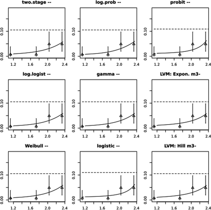
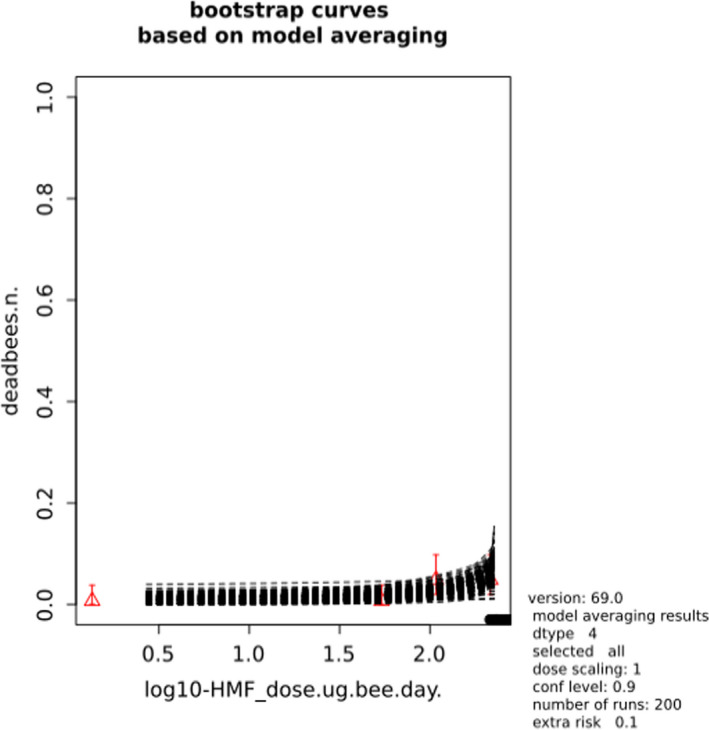
A.4. BMD analysis of larvae mortality (7 days) due to the presence of HMF in bee feed (Krainer et al., 2016)

A) Data description

The endpoint to be analysed is: number of dead larvae.

B) Data used for analysis

HMF in μg/larvae per day	Number of dead larvae	Total number of larvae
0.00	30	336
0.14	23	336
1.41	34	336
21.22	23	336
142.00	176	336
212.00	336	336
283.00	336	336

C) Selection of the BMR

The benchmark response (BMR) used is an extra risk of 10%. The benchmark dose (BMD) is the dose corresponding to the BMR of interest. A 90% confidence interval for the BMD will be estimated, with lower and upper bound denoted BMDL and BMDU, respectively.

D) Software used

Results are obtained using the EFSA web‐tool for BMD analysis, which uses the R‐package PROAST, version 69.0, for the underlying calculations.

E) Results

Response variable: number of dead larvae.

Fitted models

Model	No.par	loglik	AIC	Accepted	BMDL	BMDU	BMD	conv
null	1	–1,589.64	3,181.28		NA	NA	NA	NA
full	7	–611.46	1,236.92		NA	NA	NA	NA
two.stage	3	–667.88	1,341.76	No	NA	NA	44.1	No
log.logist	3	–613.21	1,232.42	Yes	121.0	130	136.0	Yes
Weibull	3	–613.21	1,232.42	Yes	98.6	139	115.0	Yes
log.prob	3	–613.21	1,232.42	Yes	117.0	129	131.0	Yes
gamma	3	–613.21	1,232.42	Yes	0.0	126	125.0	Yes
logistic	2	–668.79	1,341.58	No	NA	NA	43.1	Yes
probit	2	–665.09	1,334.18	No	NA	NA	37.6	Yes
LVM: Expon. m3‐	3	–613.22	1,232.44	Yes	88.4	109	106.0	Yes
LVM: Hill m3‐	3	–613.42	1,232.84	Yes	95.5	105	103.0	Yes

Estimated model parameters

two.stage

estimate for a‐ : 0.07529

estimate for BMD‐ : 44.15

estimate for c : 1e+12

log.logist

estimate for a‐ : 0.08185

estimate for BMD‐ : 135.7

estimate for c : 46.55

Weibull

estimate for a‐ : 0.08185

estimate for BMD‐ : 115.2

estimate for c : 8.76

log.prob

estimate for a‐ : 0.08185

estimate for BMD‐ : 130.6

estimate for c : 14.74

gamma

estimate for a‐ : 0.08184

estimate for BMD‐ : 125.1

estimate for c : 100

logistic

estimate for a‐ : −2.764

estimate for BMD‐ : 43.09

probit

estimate for a‐ : −1.549

estimate for BMD‐ : 37.62

EXP

estimate for a‐ : 1.417

estimate for BMD‐ : 106.1

estimate for d‐ : 4

estimate for th(fixed) : 0

estimate for sigma(fixed) : 0.25

HILL

estimate for a‐ : 1.417

estimate for BMD‐ : 102.6

estimate for d‐ : 4

estimate for th(fixed) : 0

estimate for sigma(fixed) : 0.25

Weights for model averaging

two.stage	log.logist	Weibull	log.prob	gamma	logistic	probit	EXP	HILL
0	0.17	0.17	0.17	0.17	0	0	0.17	0.14

F) Final BMD values

Subgroup	BMDL	BMDU
All	115	123

Confidence intervals for the BMD are based on 200 bootstrap data sets.

G) Visualisation

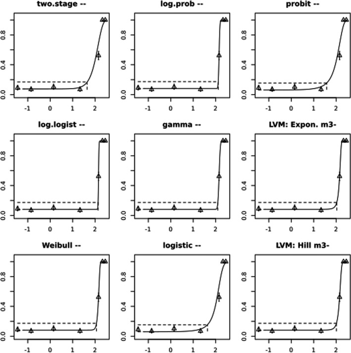
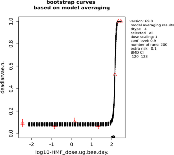
A.5. BMD analysis of bee mortality (after 22 days) due to the presence of HMF in bee feed (Krainer et al., 2016)

A) Data description

The endpoint to be analysed is: number of dead bees.

B) Data used for analysis

HMF in μg/bee per day	Number of dead bees	Total number of bees
0	10	144
54	97	144
108	144	144
216	144	144

C) Selection of the BMR

The benchmark response (BMR) used is an extra risk of 10%. The benchmark dose (BMD) is the dose corresponding to the BMR of interest. A 90% confidence interval for the BMD will be estimated, with lower and upper bound denoted BMDL and BMDU, respectively.

D) Software used

Results are obtained using the EFSA web‐tool for BMD analysis, which uses the R‐package PROAST, version 69.0, for the underlying calculations.

E) Results

Response variable: number of dead bees.

Fitted models

Model	No.par	loglik	AIC	Accepted	BMDL	BMDU	BMD	conv
null	1	–358.53	719.06		NA	NA	NA	NA
full	4	–127.27	262.54		NA	NA	NA	NA
two.stage	3	–128.95	263.90	No	NA	NA	16.4	Yes
log.logist	3	–127.27	260.54	Yes	32.6	51.3	45.2	Yes
Weibull	3	–127.27	260.54	Yes	17.2	48.5	31.5	Yes
log.prob	3	–127.27	260.54	Yes	28.9	52.3	43.7	Yes
gamma	3	–127.27	260.54	Yes	24.1	45.7	42.0	Yes
LVM: Expon. m3‐	3	–127.27	260.54	Yes	12.6	42.5	26.9	Yes
LVM: Hill m3‐	3	–127.27	260.54	Yes	12.7	37.6	27.2	Yes

Estimated model parameters

two.stage

estimate for a‐ : 0.06744

estimate for BMD‐ : 16.43

estimate for c : 1e+12

log.logist

estimate for a‐ : 0.0695

estimate for BMD‐ : 45.23

estimate for c : 15.88

Weibull

estimate for a‐ : 0.06944

estimate for BMD‐ : 31.51

estimate for c : 4.264

log.prob

estimate for a‐ : 0.06944

estimate for BMD‐ : 43.72

estimate for c : 7.88

gamma

estimate for a‐ : 0.06944

estimate for BMD‐ : 42.02

estimate for c : 46.4

EXP

estimate for a‐ : 1.448

estimate for BMD‐ : 26.87

estimate for d‐ : 1.954

estimate for th(fixed) : 0

estimate for sigma(fixed) : 0.25

HILL

estimate for a‐ : 1.448

estimate for BMD‐ : 27.23

estimate for d‐ : 1.998

estimate for th(fixed) : 0

estimate for sigma(fixed) : 0.25

Weights for model averaging

two.stage	log.logist	Weibull	log.prob	gamma	EXP	HILL
0.03	0.16	0.16	0.16	0.16	0.16	0.16

F) Final BMD Values

Subgroup	BMDL	BMDU
All	32.7	37.6

Confidence intervals for the BMD are based on 200 bootstrap data sets.

G) Visualisation

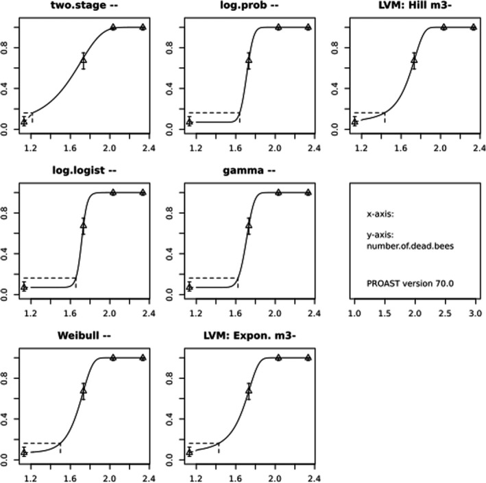
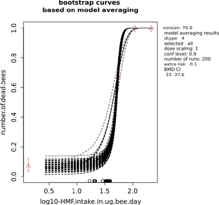
A.6. BMD analysis of larvae mortality (after 22 days) due to the presence of HMF in bee feed (Krainer et al., 2016)

A) Data description

The endpoint to be analysed is: number of dead larvae.

B) Data used for analysis

HMF in μg/larvae per day	Number of dead larvae	Total number of larvae
0.00	94	336
0.14	89	336
1.41	102	336
21.22	108	336
142.00	294	336
212.00	336	336
283.00	336	336

C) Selection of the BMR

The benchmark response (BMR) used is an extra risk of 10%. The benchmark dose (BMD) is the dose corresponding to the BMR of interest. A 90% confidence interval for the BMD will be estimated, with lower and upper bound denoted BMDL and BMDU, respectively.

D) Software used

Results are obtained using the EFSA web‐tool for BMD analysis, which uses the R‐package PROAST, version 69.0, for the underlying calculations.

E) Results

Response variable: number of dead larvae.

Fitted models

Model	No.par	Loglik	AIC	Accepted	BMDL	BMDU	BMD	conv
Null	1	–1601.69	3,205.38		NA	NA	NA	NA
Full	7	–937.24	1,888.48		NA	NA	NA	NA
two.stage	3	–942.05	1,890.10	No	NA	NA	33.2	No
log.logist	3	–938.77	1,883.54	Yes	93.9	101.0	130.0	Yes
Weibull	3	–938.76	1,883.52	Yes	45.6	132.0	77.4	Yes
log.prob	3	–938.77	1,883.54	Yes	80.5	139.0	118.0	Yes
gamma	3	–938.77	1,883.54	Yes	71.6	114.0	114.0	No
logistic	2	–949.95	1,903.90	No	NA	NA	15.2	Yes
probit	2	–945.52	1,895.04	No	NA	NA	15.8	Yes
LVM: Expon. m3‐	3	–938.44	1,882.88	Yes	30.1	81.3	49.7	Yes
LVM: Hill m3‐	3	–938.73	1,883.46	Yes	39.3	81.0	67.7	Yes

Estimated model parameters

two.stage

estimate for a‐ : 0.2837

estimate for BMD‐ : 33.16

estimate for c : 55920000

log.logist

estimate for a‐ : 0.2924

estimate for BMD‐ : 129.7

estimate for c : 41.15

Weibull

estimate for a‐ : 0.2924

estimate for BMD‐ : 77.45

estimate for c : 4.62

log.prob

estimate for a‐ : 0.2924

estimate for BMD‐ : 117.6

estimate for c : 11.71

gamma

estimate for a‐ : 0.2924

estimate for BMD‐ : 113.7

estimate for c : 100

logistic

estimate for a‐ : −1.033

estimate for BMD‐ : 15.19

probit

estimate for a‐ : −0.6296

estimate for BMD‐ : 15.79

EXP

estimate for a‐ : 1.149

estimate for BMD‐ : 49.66

estimate for d‐ : 2.055

estimate for th(fixed) : 0

estimate for sigma(fixed) : 0.25

HILL

estimate for a‐ : 1.147

estimate for BMD‐ : 67.73

estimate for d‐ : 3.178

estimate for th(fixed) : 0

estimate for sigma(fixed) : 0.25

Weights for model averaging

two.stage	log.logist	Weibull	log.prob	Gamma	logistic	probit	EXP	HILL
0.01	0.15	0.16	0.15	0.15	0	0	0.21	0.16

F) Final BMD values

Subgroup	BMDL	BMDU
All	64.3	102

Confidence intervals for the BMD are based on 200 bootstrap data sets.

G) Visualisation

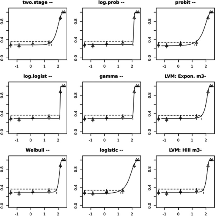
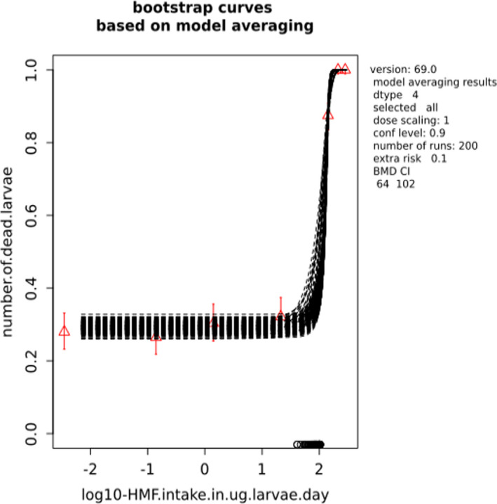
A.7. BMC analysis of bee mortality (after 22 days) due to the presence of HMF in bee feed (Krainer et al., 2016)

A) Data description

The endpoint to be analysed is: number of dead bees.

B) Data used for analysis

HMF in mg/kg feed	Number of dead bees	Total number of bees
0	10	144
2,000	97	144
4,000	144	144
8,000	144	144

C) Selection of the BMR

The benchmark response (BMR) used is an extra risk of 10%. The benchmark concentration (BMC) is the concentration corresponding to the BMR of interest. A 90% confidence interval for the BMC will be estimated, with lower and upper bound denoted BMCL and BMCU, respectively.

D) Software used

Results are obtained using the EFSA web‐tool for BMC analysis, which uses the R‐package PROAST, version 69.0, for the underlying calculations.

E) Results

Response variable: number of dead bees.

Fitted models

Model	No.par	loglik	AIC	Accepted	BMCL	BMCU	BMD	conv
Null	1	–3.5853e+02	7.1906e+02		NA	NA	NA	NA
Full	4	–1.2727e+02	2.6254e+02		NA	NA	NA	NA
two.stage	3	–1.2895e+02	2.6390e+02	No	NA	NA	6.08e+02	Yes
log.logist	3	–1.2727e+02	2.6054e+02	Yes	1210	1900	1.68e+03	Yes
Weibull	3	–1.2727e+02	2.6054e+02	Yes	635	1940	1.17e+03	Yes
log.prob	3	–1.2727e+02	2.6054e+02	Yes	1070	1740	1.62e+03	Yes
gamma	3	–1.2727e+02	2.6054e+02	Yes	893	1570	1.55e+03	Yes
logistic	2	–1.2928e+02	2.6256e+02	No	NA	NA	5.92e+02	Yes
probit	2	–1.0000e+10	2.0000e+10	No	NA	NA	2.80e+08	Yes
LVM: Expon. m3‐	3	–1.2727e+02	2.6054e+02	Yes	465	1480	9.93e+02	Yes
LVM: Hill m3‐	3	–1.2727e+02	2.6054e+02	Yes	609	1420	1.21e+03	Yes

Estimated model parameters

two.stage

estimate for a‐ : 0.06744

estimate for BMD‐ : 608.3

estimate for c : 1e+12

log.logist

estimate for a‐ : 0.0695

estimate for BMD‐ : 1675

estimate for c : 15.88

Weibull

estimate for a‐ : 0.06944

estimate for BMD‐ : 1172

estimate for c : 4.296

log.prob

estimate for a‐ : 0.06944

estimate for BMD‐ : 1617

estimate for c : 7.834

gamma

estimate for a‐ : 0.06944

estimate for BMD‐ : 1554

estimate for c : 45.9

logistic

estimate for a‐ : −2.789

estimate for BMD‐ : 591.7

probit

estimate for a‐ : −0.7854

estimate for BMD‐ : 280400000

EXP

estimate for a‐ : 1.448

estimate for BMD‐ : 993.3

estimate for d‐ : 1.942

estimate for th(fixed) : 0

estimate for sigma(fixed) : 0.25

HILL

estimate for a‐ : 1.448

estimate for BMD‐ : 1209

estimate for d‐ : 3.076

estimate for th(fixed) : 0

estimate for sigma(fixed) : 0.25

Weights for model averaging

two.stage	log.logist	Weibull	log.prob	gamma	logistic	probit	EXP	HILL
0.03	0.15	0.15	0.15	0.15	0.06	0	0.15	0.15

F) Final BMC Values

Subgroup	BMCL	BMCU
All	745	1410

Confidence intervals for the BMC are based on 200 bootstrap data sets.

G) Visualisation

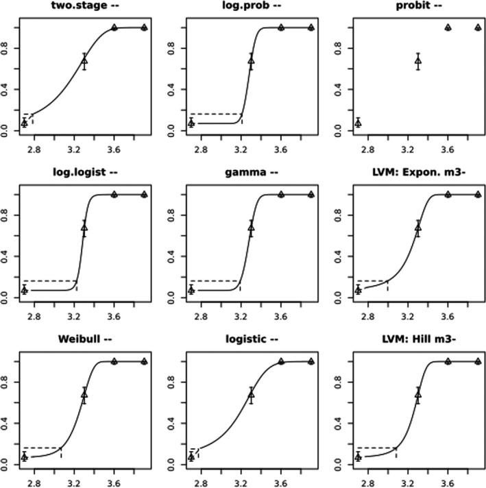
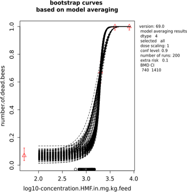
A.8. BMC analysis of bee mortality (after 7 days) due to the presence of HMF in bee feed (Krainer et al., 2016)

A) Data description

The endpoint to be analysed is: number of dead bees.

B) Data used for analysis

HMF in mg/kg feed	Number of dead bees	Total number of bees
0	1	144
2,000	1	144
4,000	7	144
8,000	7	144

C) Selection of the BMR

The benchmark response (BMR) used is an extra risk of 10%. The benchmark concentration (BMC) is the concentration corresponding to the BMR of interest. A 90% confidence interval for the BMC will be estimated, with lower and upper bound denoted BMCL and BMCU, respectively.

D) Software used

Results are obtained using the EFSA web‐tool for BMC analysis, which uses the R‐package PROAST, version 69.0, for the underlying calculations.

E) Results

Response variable: number of dead bees.

Fitted models

Model	No.par	loglik	AIC	Accepted	BMCL	BMCU	BMD	conv
null	1	–7.311e+01	1.4822e+02		NA	NA	NA	NA
full	4	–6.792e+01	1.4384e+02		NA	NA	NA	NA
two.stage	3	–6.933e+01	1.4466e+02	Yes	10100	38700	1.64e+04	Yes
log.logist	3	–6.932e+01	1.4464e+02	Yes	8710	65100000	1.57e+04	Yes
Weibull	3	–6.933e+01	1.4466e+02	Yes	8700	90600000	1.55e+04	Yes
log.prob	3	–6.924e+01	1.4448e+02	Yes	8740	33400000	1.65e+04	Yes
gamma	3	–6.933e+01	1.4466e+02	Yes	8690	79600000	1.54e+04	Yes
logistic	2	–7.311e+01	1.5022e+02	No	NA	NA	1.07e+07	Yes
probit	2	–1.000e+10	2.0000e+10	No	NA	NA	1.11e+09	Yes
LVM: Expon. m3‐	3	–6.945e+01	1.4490e+02	Yes	8670	312000	1.46e+04	Yes
LVM: Hill m3‐	3	–6.943e+01	1.4486e+02	Yes	8680	401000	1.49e+04	Yes

Estimated model parameters

two.stage

estimate for a‐ : 0.005853

estimate for BMD‐ : 16410

estimate for c : 1e‐06

log.logist

estimate for a‐ : 0.005951

estimate for BMD‐ : 15680

estimate for c : 1.078

Weibull

estimate for a‐ : 0.00596

estimate for BMD‐ : 15520

estimate for c : 1.058

log.prob

estimate for a‐ : 0.005942

estimate for BMD‐ : 16490

estimate for c : 0.4779

gamma

estimate for a‐ : 0.005976

estimate for BMD‐ : 15420

estimate for c : 1.071

logistic

estimate for a‐ : −3.556

estimate for BMD‐ : 10730000

probit

estimate for a‐ : −2.488

estimate for BMD‐ : 1.106e+09

EXP

estimate for a‐ : 1.875

estimate for BMD‐ : 14600

estimate for d‐ : 0.5246

estimate for th(fixed) : 0

estimate for sigma(fixed) : 0.25

HILL

estimate for a‐ : 1.876

estimate for BMD‐ : 14860

estimate for d‐ : 0.5773

estimate for th(fixed) : 0

estimate for sigma(fixed) : 0.25

Weights for model averaging

two.stage	log.logist	Weibull	log.prob	gamma	logistic	probit	EXP	HILL
0.14	0.15	0.14	0.16	0.14	0.01	0	0.13	0.13

F) Final BMC values

Subgroup	BMCL	BMCU
All	8420	227000

Confidence intervals for the BMC are based on 200 bootstrap data sets.

G) Visualisation

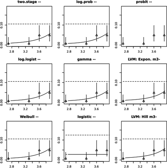
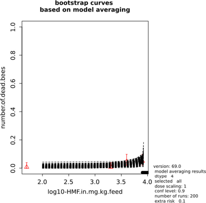
A.9. BMC analysis of larvae mortality (after 22 days) due to the presence of HMF in bee feed (Krainer et al., 2016)

A) Data description

The endpoint to be analysed is: number of dead larvae.

B) Data used for analysis

HMF in mg/kg feed	Number of dead larvae	Total number of larvae
0	94	336
5	89	336
50	102	336
750	108	336
5,000	294	336
7,500	336	336
10,000	336	336

C) Selection of the BMR

The benchmark response (BMR) used is an extra risk of 10%. The benchmark concentration (BMC) is the concentration corresponding to the BMR of interest. A 90% confidence interval for the BMC will be estimated, with lower and upper bound denoted BMCL and BMCU, respectively.

D) Software used

Results are obtained using the EFSA web‐tool for BMC analysis, which uses the R‐package PROAST, version 69.0, for the underlying calculations.

E) Results

Response variable: number of dead larvae.

Fitted models

model	No.par	loglik	AIC	accepted	BMCL	BMCU	BMD	conv
null	1	–1.60169e+03	3.20538e+03		NA	NA	NA	NA
Full	7	–9.37240e+02	1.88848e+03		NA	NA	NA	NA
two.stage	3	–9.41910e+02	1.88982e+03	No	NA	NA	1.17e+03	No
log.logist	3	–9.38770e+02	1.88354e+03	Yes	3290	3560	4.55e+03	Yes
Weibull	3	–9.38760e+02	1.88352e+03	Yes	1570	4790	2.69e+03	Yes
log.prob	3	–9.38770e+02	1.88354e+03	Yes	2810	4890	4.13e+03	Yes
gamma	3	–9.38770e+02	1.88354e+03	Yes	2500	3210	4.00e+03	No
logistic	2	–9.49790e+02	1.90358e+03	No	NA	NA	5.36e+02	Yes
probit	2	–1.00000e+10	2.00000e+10	No	NA	NA	4.03e+08	Yes
LVM: Expon. m3‐	3	–9.38410e+02	1.88282e+03	Yes	1050	2950	1.72e+03	Yes
LVM: Hill m3‐	3	–9.38720e+02	1.88344e+03	Yes	1360	2850	2.34e+03	Yes

Estimated Model Parameters

two.stage

estimate for a‐ : 0.2837

estimate for BMD‐ : 1169

estimate for c : 1e+12

log.logist

estimate for a‐ : 0.2924

estimate for BMD‐ : 4550

estimate for c : 39.61

Weibull

estimate for a‐ : 0.2923

estimate for BMD‐ : 2689

estimate for c : 4.517

log.prob

estimate for a‐ : 0.2924

estimate for BMD‐ : 4133

estimate for c : 11.61

gamma

estimate for a‐ : 0.2924

estimate for BMD‐ : 4002

estimate for c : 100

logistic

estimate for a‐ : −1.033

estimate for BMD‐ : 535.9

probit

estimate for a‐ : −0.5721

estimate for BMD‐ : 403100000

EXP

estimate for a‐ : 1.149

estimate for BMD‐ : 1722

estimate for d‐ : 2.026

estimate for th(fixed) : 0

estimate for sigma(fixed) : 0.25

HILL

estimate for a‐ : 1.147

estimate for BMD‐ : 2344

estimate for d‐ : 3.107

estimate for th(fixed) : 0

estimate for sigma(fixed) : 0.25

Weights for model averaging

two.stage	log.logist	Weibull	log.prob	gamma	logistic	probit	EXP	HILL
0.01	0.15	0.15	0.15	0.15	0	0	0.22	0.16

F) Final BMC values

Subgroup	BMCL	BMCU
All	2130	3600

Confidence intervals for the BMC are based on 200 bootstrap data sets.

G) Visualisation

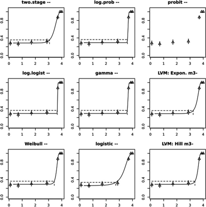
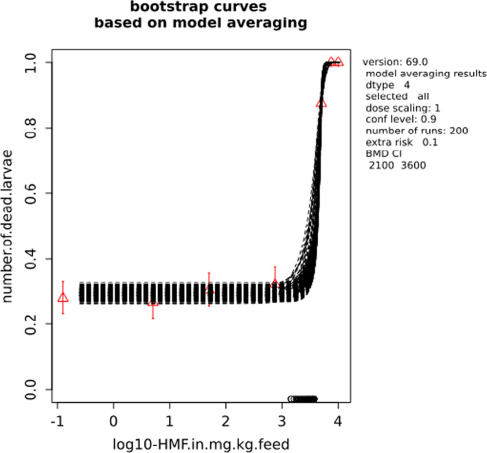
A.10. BMC analysis of larvae mortality (after 7 days) due to the presence of HMF in bee feed (Krainer et al., 2016)

A) Data description

The endpoint to be analysed is: number of dead larvae.

B) Data used for analysis

HMF in mg/kg feed	Number of dead larvae	Total number of larvae
0	30	336
5	23	336
50	34	336
750	23	336
5,000	176	336
7,500	336	336
10,000	336	336

C) Selection of the BMR

The benchmark response (BMR) used is an extra risk of 10%. The benchmark concentration (BMC) is the concentration corresponding to the BMR of interest. A 90% confidence interval for the BMC will be estimated, with lower and upper bound denoted BMCL and BMCU, respectively.

D) Software used

Results are obtained using the EFSA web‐tool for BMC analysis, which uses the R‐package PROAST, version 69.0, for the underlying calculations.

E) Results

Response variable: number of dead larvae.

Fitted models

Model	No.par	loglik	AIC	Accepted	BMCL	BMCU	BMD	conv
null	1	–1.58964e+03	3.18128e+03		NA	NA	NA	NA
Full	7	–6.11460e+02	1.23692e+03		NA	NA	NA	NA
two.stage	3	–6.67090e+02	1.34018e+03	No	NA	NA	1.56e+03	Yes
log.logist	3	–6.13210e+02	1.23242e+03	Yes	4260	4580	4.77e+03	Yes
Weibull	3	–6.13210e+02	1.23242e+03	Yes	3460	4870	4.05e+03	Yes
log.prob	3	–6.13210e+02	1.23242e+03	Yes	4120	4670	4.59e+03	Yes
gamma	3	–6.13210e+02	1.23242e+03	Yes	0	4420	4.41e+03	Yes
logistic	2	–6.68020e+02	1.34004e+03	No	NA	NA	1.52e+03	Yes
probit	2	–1.00000e+10	2.00000e+10	No	NA	NA	3.21e+08	Yes
LVM: Expon. m3‐	3	–6.13220e+02	1.23244e+03	Yes	3100	3830	3.74e+03	Yes
LVM: Hill m3‐	3	–6.13390e+02	1.23278e+03	Yes	3350	3700	3.61e+03	Yes

Estimated model parameters

two.stage

estimate for a‐ : 0.07528

estimate for BMD‐ : 1557

estimate for c : 1e+12

log.logist

estimate for a‐ : 0.08185

estimate for BMD‐ : 4774

estimate for c : 45.8

Weibull

estimate for a‐ : 0.08185

estimate for BMD‐ : 4049

estimate for c : 8.676

log.prob

estimate for a‐ : 0.08185

estimate for BMD‐ : 4592

estimate for c : 14.5

gamma

estimate for a‐ : 0.08184

estimate for BMD‐ : 4406

estimate for c : 100

logistic

estimate for a‐ : −2.764

estimate for BMD‐ : 1520

probit

estimate for a‐ : −1.492

estimate for BMD‐ : 3.21e+08

EXP

estimate for a‐ : 1.417

estimate for BMD‐ : 3737

estimate for d‐ : 4

estimate for th(fixed) : 0

estimate for sigma(fixed) : 0.25

HILL

estimate for a‐ : 1.417

estimate for BMD‐ : 3613

estimate for d‐ : 4

estimate for th(fixed) : 0

estimate for sigma(fixed) : 0.25

Weights for model averaging

two.stage	log.logist	Weibull	log.prob	gamma	logistic	probit	EXP	HILL
0	0.17	0.17	0.17	0.17	0	0	0.17	0.14

F) Final BMC values

Subgroup	BMCL	BMCU
All	4090	4320

Confidence intervals for the BMC are based on 200 bootstrap data sets.

G) Visualisation

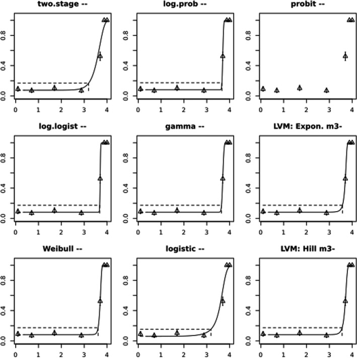
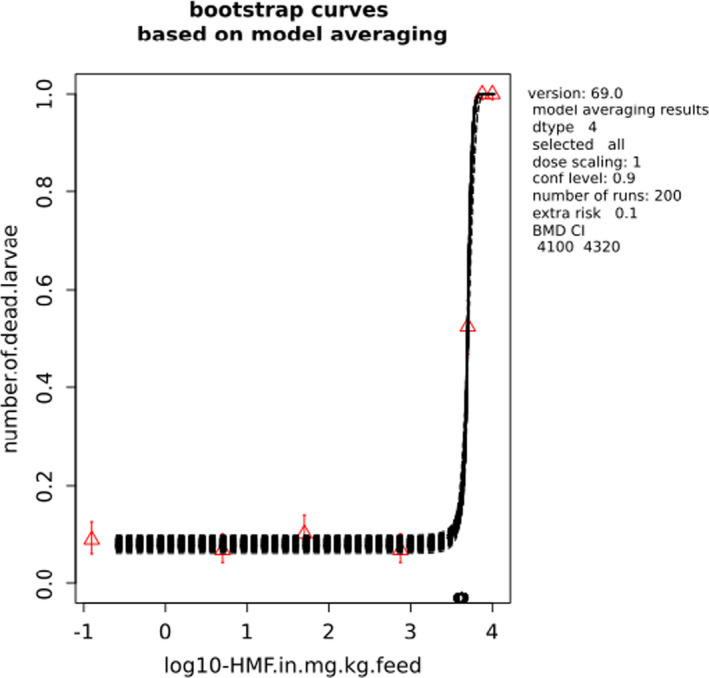
A.11. BMD analysis of bee mortality (after 15 days) due to the presence of HMF in bee feed (Gregorc et al., 2020)

A) Data description

The endpoint to be analysed is: number of dead bees.

B) Data used for analysis

HMF in μg/bee per day	Number of dead bees	Total number of bees
0.0	8	350
1.5	16	350
7.5	11	350
15.0	14	350
22.5	28	350

C) Selection of the BMR

The benchmark response (BMR) used is an extra risk of 10%. The benchmark dose (BMD) is the dose corresponding to the BMR of interest. A 90% confidence interval for the BMD will be estimated, with lower and upper bound denoted BMDL and BMDU, respectively.

D) Software used

Results are obtained using the EFSA web‐tool for BMD analysis, which uses the R‐package PROAST, version 69.0, for the underlying calculations.

E) Results

Response variable: number of dead bees.

Fitted models

Model	No.par	loglik	AIC	Accepted	BMDL	BMDU	BMD	conv
null	1	–315.80	633.60		NA	NA	NA	NA
full	5	–308.37	626.74		NA	NA	NA	NA
two.stage	3	–310.47	626.94	Yes	27.5	50.5	34.7	No
log.logist	3	–309.81	625.62	Yes	22.6	54.1	26.3	Yes
Weibull	3	–309.81	625.62	Yes	22.7	53.1	26.2	Yes
log.prob	3	–309.80	625.60	Yes	23.1	58.6	27.2	Yes
gamma	3	–309.80	625.60	Yes	22.9	53.4	26.8	Yes
logistic	2	–310.89	625.78	Yes	27.7	69.9	37.6	Yes
probit	2	–310.97	625.94	Yes	28.7	76.8	39.8	No
LVM: Expon. m3‐	3	–309.81	625.62	Yes	23.5	49.4	25.5	Yes
LVM: Hill m3‐	3	–309.81	625.62	Yes	23.6	49.8	25.7	Yes

Estimated model parameters

two.stage

estimate for a‐ : 0.03083

estimate for BMD‐ : 34.68

estimate for c : 1e+12

log.logist

estimate for a‐ : 0.03332

estimate for BMD‐ : 26.33

estimate for c : 4.984

Weibull

estimate for a‐ : 0.03332

estimate for BMD‐ : 26.22

estimate for c : 4.933

log.prob

estimate for a‐ : 0.03334

estimate for BMD‐ : 27.24

estimate for c : 1.987

gamma

estimate for a‐ : 0.03333

estimate for BMD‐ : 26.81

estimate for c : 7.185

logistic

estimate for a‐ : −3.532

estimate for BMD‐ : 37.61

probit

estimate for a‐ : −1.905

estimate for BMD‐ : 39.83

EXP

estimate for a‐ : 1.582

estimate for BMD‐ : 25.49

estimate for d‐ : 4

estimate for th(fixed) : 0

estimate for sigma(fixed) : 0.25

HILL

estimate for a‐ : 1.583

estimate for BMD‐ : 25.71

estimate for d‐ : 4

estimate for th(fixed) : 0

estimate for sigma(fixed) : 0.25

Weights for model averaging

two.stage	log.logist	Weibull	log.prob	gamma	logistic	probit	EXP	HILL
0.06	0.12	0.12	0.12	0.12	0.11	0.1	0.12	0.12

F) Final BMD values

Subgroup	BMDL	BMDU
All	23.3	58.7

Confidence intervals for the BMD are based on 200 bootstrap data sets.

G) Visualisation

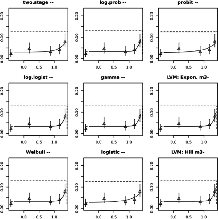
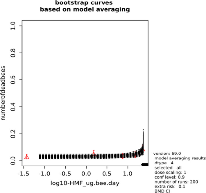
A.12. BMD analysis of bee mortality (after 20 days) due to the presence of HMF in bee feed (Gregorc et al., 2020)

A) Data description

The endpoint to be analysed is: number of dead bees.

B) Data used for analysis

HMF in μg/bee per day	Number of dead bees	Total number of bees
0.0	29	350
1.5	40	350
7.5	43	350
15.0	43	350
22.5	87	350

C) Selection of the BMR

The benchmark response (BMR) used is an extra risk of 10%. The benchmark dose (BMD) is the dose corresponding to the BMR of interest. A 90% confidence interval for the BMD will be estimated, with lower and upper bound denoted BMDL and BMDU, respectively.

D) Software used

Results are obtained using the EFSA web‐tool for BMD analysis, which uses the R‐package PROAST, version 69.0, for the underlying calculations.

E) Results

Response variable: number of dead bees.

Fitted models

Model	No.par	loglik	AIC	Accepted	BMDL	BMDU	BMD	conv
null	1	–703.22	1408.44		NA	NA	NA	NA
full	5	–681.45	1372.90		NA	NA	NA	NA
two.stage	3	–684.69	1375.38	no	NA	NA	18.4	Yes
log.logist	3	–683.11	1372.22	Yes	17.8	22.8	20.4	Yes
Weibull	3	–683.11	1372.22	Yes	17.8	22.5	20.5	Yes
log.prob	3	–683.13	1372.26	Yes	17.9	22.5	20.3	Yes
gamma	3	–683.13	1372.26	Yes	17.8	22.3	20.3	Yes
LVM: Expon. m3‐	3	–683.09	1372.18	Yes	17.6	22.0	20.6	Yes
LVM: Hill m3‐	3	–683.17	1372.34	Yes	17.5	21.7	20.1	Yes

Estimated model parameters

two.stage

estimate for a‐ : 0.09634

estimate for BMD‐ : 18.35

estimate for c : 1e+12

log.logist

estimate for a‐ : 0.1062

estimate for BMD‐ : 20.43

estimate for c : 5.502

Weibull

estimate for a‐ : 0.1061

estimate for BMD‐ : 20.48

estimate for c : 5.278

log.prob

estimate for a‐ : 0.1066

estimate for BMD‐ : 20.25

estimate for c : 2.686

gamma

estimate for a‐ : 0.1065

estimate for BMD‐ : 20.33

estimate for c : 10.2

EXP

estimate for a‐ : 1.367

estimate for BMD‐ : 20.6

estimate for d‐ : 4.287

estimate for th(fixed) : 0

estimate for sigma(fixed) : 0.25

HILL

estimate for a‐ : 1.371

estimate for BMD‐ : 20.09

estimate for d‐ : 3.333

estimate for th(fixed) : 0

estimate for sigma(fixed) : 0.25

Weights for model averaging

two.stage	log.logist	Weibull	log.prob	gamma	EXP	HILL
0.03	0.16	0.16	0.16	0.16	0.17	0.15

F) Final BMD values

Subgroup	BMDL	BMDU
All	18	22.2

Confidence intervals for the BMD are based on 200 bootstrap data sets.

G) Visualisation

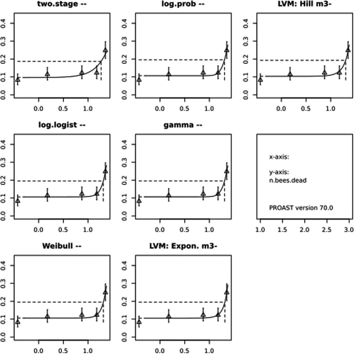
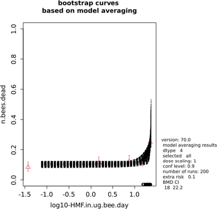
A.13. BMC analysis of bee mortality (after 20 days) due to the presence of HMF in bee feed (Gregorc et al., 2020)

A) Data description

The endpoint to be analysed is: number of dead bees.

B) Data used for analysis

HMF in mg/kg feed	Number of dead bees	Total number of bees
0	29	350
100	40	350
500	43	350
1,000	43	350
1,500	87	350

C) Selection of the BMR

The benchmark response (BMR) used is an extra risk of 10%. The benchmark concentration (BMC) is the concentration corresponding to the BMR of interest. A 90% confidence interval for the BMC will be estimated, with lower and upper bound denoted BMCL and BMCU, respectively.

D) Software used

Results are obtained using the EFSA web‐tool for BMC analysis, which uses the R‐package PROAST, version 69.0, for the underlying calculations.

E) Results

Response variable: number of dead bees.

Fitted models

Model	No.par	loglik	AIC	Accepted	BMCL	BMCU	BMD	conv
null	1	–7.0322e+02	1.40844e+03		NA	NA	NA	NA
full	5	–6.8145e+02	1.37290e+03		NA	NA	NA	NA
two.stage	3	–6.8469e+02	1.37538e+03	No	NA	NA	1.22e+03	Yes
log.logist	3	–6.8311e+02	1.37222e+03	Yes	1190	1520	1.36e+03	Yes
Weibull	3	–6.8311e+02	1.37222e+03	Yes	1190	1500	1.36e+03	Yes
log.prob	3	–6.8313e+02	1.37226e+03	Yes	1200	1500	1.35e+03	Yes
gamma	3	–6.8313e+02	1.37226e+03	Yes	1190	1490	1.36e+03	Yes
logistic	2	–7.0309e+02	1.41018e+03	No	NA	NA	2.21e+05	Yes
probit	2	–1.0000e+10	2.00000e+10	No	NA	NA	3.51e+08	Yes
LVM: Expon. m3–	3	–6.8309e+02	1.37218e+03	Yes	1180	1460	1.36e+03	Yes
LVM: Hill m3‐	3	–6.8311e+02	1.37222e+03	Yes	1180	1450	1.36e+03	Yes

Estimated model parameters

two.stage

estimate for a‐ : 0.09634

estimate for BMD‐ : 1223

estimate for c : 1e+12

log.logist

estimate for a‐ : 0.1062

estimate for BMD‐ : 1362

estimate for c : 5.502

Weibull

estimate for a‐ : 0.1061

estimate for BMD‐ : 1365

estimate for c : 5.278

log.prob

estimate for a‐ : 0.1066

estimate for BMD‐ : 1350

estimate for c : 2.686

gamma

estimate for a‐ : 0.1065

estimate for BMD‐ : 1355

estimate for c : 10.2

logistic

estimate for a‐ : −1.831

estimate for BMD‐ : 220600

probit

estimate for a‐ : −1.354

estimate for BMD‐ : 351400000

EXP

estimate for a‐ : 1.368

estimate for BMD‐ : 1365

estimate for d‐ : 4

estimate for th(fixed) : 0

estimate for sigma(fixed) : 0.25

HILL

estimate for a‐ : 1.368

estimate for BMD‐ : 1357

estimate for d‐ : 4

estimate for th(fixed) : 0

estimate for sigma(fixed) : 0.25

Weights for model averaging

two.stage	log.logist	Weibull	log.prob	gamma	logistic	probit	EXP	HILL
0.03	0.16	0.16	0.16	0.16	0	0	0.16	0.16

F) Final BMC values

Subgroup	BMCL	BMCU
All	1200	1480

Confidence intervals for the BMC are based on 200 bootstrap data sets.

G) Visualisation

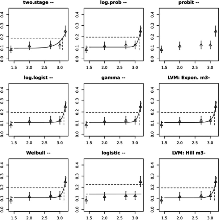
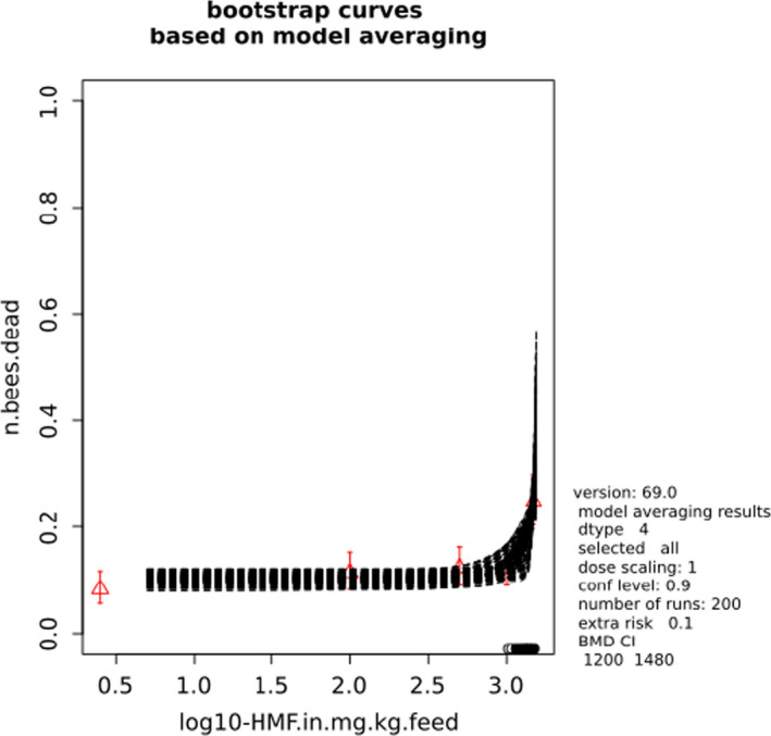
A.14. BMC analysis of bee mortality (after 15 days) due to the presence of HMF in bee feed (Gregorc et al., 2020)

A) Data description

The endpoint to be analysed is: number of dead bees.

B) Data used for analysis

HMF in mg/kg feed	Number of dead bees	Total number of bees
0	8	350
100	16	350
500	11	350
1,000	16	350
1,500	28	350

C) Selection of the BMR

The benchmark response (BMR) used is an extra risk of 10%. The benchmark concentration (BMC) is the concentration corresponding to the BMR of interest. A 90% confidence interval for the BMC will be estimated, with lower and upper bound denoted BMCL and BMCU, respectively.

D) Software used

Results are obtained using the EFSA web‐tool for BMC analysis, which uses the R‐package PROAST, version 69.0, for the underlying calculations.

E) Results

Response variable: number of dead bees.

Fitted models

Model	No.par	Loglik	AIC	Accepted	BMCL	BMCU	BMD	conv
null	1	–3.2193e+02	6.4586e+02		NA	NA	NA	NA
full	5	–3.1458e+02	6.3916e+02		NA	NA	NA	NA
two.stage	3	–3.1634e+02	6.3868e+02	yes	1800	3240	2.25e+03	no
log.logist	3	–3.1604e+02	6.3808e+02	yes	1510	8920	1.87e+03	yes
Weibull	3	–3.1604e+02	6.3808e+02	yes	1520	9200	1.86e+03	yes
log.prob	3	–3.1603e+02	6.3806e+02	yes	1520	6560	1.95e+03	yes
gamma	3	–3.1604e+02	6.3808e+02	yes	1540	9420	1.90e+03	yes
logistic	2	–3.2187e+02	6.4774e+02	no	NA	NA	3.80e+05	yes
probit	2	–1.0000e+10	2.0000e+10	no	NA	NA	4.49e+08	yes
LVM: Expon. m3‐	3	–3.1606e+02	6.3812e+02	yes	1570	11800	1.78e+03	yes
LVM: Hill m3‐	3	–3.1605e+02	6.3810e+02	yes	1580	11400	1.80e+03	yes

Estimated model parameters

two.stage

estimate for a‐ : 0.03131

estimate for BMD‐ : 2255

estimate for c : 1e+12

log.logist

estimate for a‐ : 0.03319

estimate for BMD‐ : 1869

estimate for c : 3.527

Weibull

estimate for a‐ : 0.03319

estimate for BMD‐ : 1859

estimate for c : 3.484

log.prob

estimate for a‐ : 0.03327

estimate for BMD‐ : 1946

estimate for c : 1.45

gamma

estimate for a‐ : 0.03324

estimate for BMD‐ : 1899

estimate for c : 4.473

logistic

estimate for a‐ : −3.054

estimate for BMD‐ : 380400

probit

estimate for a‐ : −1.913

estimate for BMD‐ : 448900000

EXP

estimate for a‐ : 1.583

estimate for BMD‐ : 1785

estimate for d‐ : 2.84

estimate for th(fixed) : 0

estimate for sigma(fixed) : 0.25

HILL

estimate for a‐ : 1.583

estimate for BMD‐ : 1797

estimate for d‐ : 2.926

estimate for th(fixed) : 0

estimate for sigma(fixed) : 0.25

Weights for model averaging

two.stage	log.logist	Weibull	log.prob	gamma	logistic	probit	EXP	HILL
0.11	0.15	0.15	0.15	0.15	0	0	0.15	0.15

F) Final BMC values

Subgroup	BMCL	BMCU
All	1550	7320

Confidence intervals for the BMC are based on 200 bootstrap data sets.

G) Visualisation

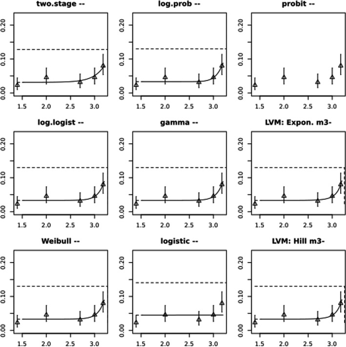
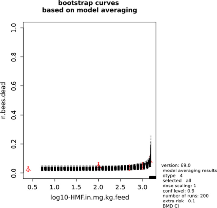
A.15. BMC analysis of bee mortality (after 30 days) due to the presence of HMF in bee feed (Luken and von der Ohe, 2016)

A) Data description

The endpoint to be analysed is: number of dead bees.

B) Data used for analysis

HMF in mg/kg feed	Number of dead bees	Total number of bees
0	37	200
40	11	80
120	17	80
240	15	80
480	22	80
960	36	80
1,920	62	80
3,840	78	80

C) Selection of the BMR

The benchmark response (BMR) used is an extra risk of 10%. The benchmark concentration (BMC) is the concentration corresponding to the BMR of interest. A 90% confidence interval for the BMC will be estimated, with lower and upper bound denoted BMCL and BMCU, respectively.

D) Software used

Results are obtained using the EFSA web‐tool for BMC analysis, which uses the R‐package PROAST, version 70.0, for the underlying calculations.

E) Results

Response variable: number of dead bees.

Fitted models

Model	No.par	loglik	AIC	Accepted	BMCL	BMCU	BMD	conv
null	1	–499.07	1000.14		NA	NA	NA	NA
full	8	–361.91	739.82		NA	NA	NA	NA
two.stage	3	–363.25	732.50	Yes	232	574	360	Yes
log.logist	3	–363.36	732.72	Yes	392	719	543	Yes
Weibull	3	–362.83	731.66	Yes	278	557	403	Yes
log.prob	3	–363.19	732.38	Yes	397	712	541	Yes
gamma	3	–362.71	731.42	Yes	306	635	457	Yes
LVM: Expon. m3‐	3	–363.56	733.12	Yes	208	460	318	Yes
LVM: Hill m3‐	3	–363.54	733.08	Yes	209	461	319	Yes

Estimated model parameters

two.stage

estimate for a‐ : 0.168

estimate for BMD‐ : 359.6

estimate for c : 4.454

log.logist

estimate for a‐ : 0.1831

estimate for BMD‐ : 542.9

estimate for c : 2.625

Weibull

estimate for a‐ : 0.1725

estimate for BMD‐ : 403.3

estimate for c : 1.578

log.prob

estimate for a‐ : 0.1841

estimate for BMD‐ : 540.7

estimate for c : 1.528

gamma

estimate for a‐ : 0.1772

estimate for BMD‐ : 457

estimate for c : 2.309

EXP

estimate for a‐ : 1.277

estimate for BMD‐ : 318

estimate for d‐ : 0.949

estimate for th(fixed) : 0

estimate for sigma(fixed) : 0.25

HILL

estimate for a‐ : 1.277

estimate for BMD‐ : 319.3

estimate for d‐ : 0.9539

estimate for th(fixed) : 0

estimate for sigma(fixed) : 0.25

Weights for model averaging

two.stage	log.logist	Weibull	log.prob	gamma	EXP	HILL
0.13	0.12	0.2	0.14	0.22	0.1	0.1

F) Final BMC Values

Subgroup	BMCL	BMCU
All	262	635

Confidence intervals for the BMC are based on 200 bootstrap data sets.

G) Visualisation

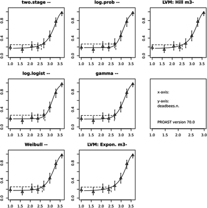
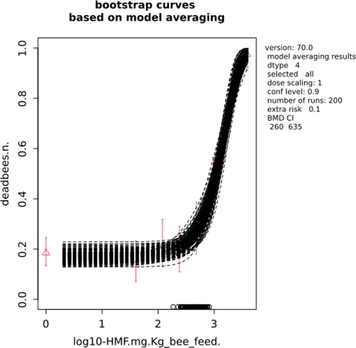
A.16. BMD analysis of bee mortality (after 30 days) due to the presence of HMF in bee feed (Luken and von der Ohe, 2016)

A) Data description

The endpoint to be analysed is: number of dead bees.

B) Data used for analysis

HMF in μg/bee per day	Number of dead bees	Total number of bees
0.00	37	200
0.90	11	80
2.71	17	80
5.42	15	80
10.84	22	80
21.69	36	80
43.37	62	80
86.75	78	80

C) Selection of the BMR

The benchmark response (BMR) used is an extra risk of 10%. The benchmark dose (BMD) is the dose corresponding to the BMR of interest. A 90% confidence interval for the BMD will be estimated, with lower and upper bound denoted BMDL and BMDU, respectively.

D) Software used

Results are obtained using the EFSA web‐tool for BMD analysis, which uses the R‐package PROAST, version 70.0, for the underlying calculations.

E) Results

Response variable: number of dead bees.

Fitted models

Model	No.par	loglik	AIC	Accepted	BMDL	BMDU	BMD	conv
null	1	–499.07	1000.14		NA	NA	NA	NA
full	8	–361.91	739.82		NA	NA	NA	NA
two.stage	3	–363.25	732.50	Yes	5.24	13.0	8.12	Yes
log.logist	3	–363.36	732.72	Yes	8.85	16.2	12.30	Yes
Weibull	3	–362.83	731.66	Yes	6.27	12.6	9.11	Yes
log.prob	3	–363.19	732.38	Yes	8.97	16.1	12.20	Yes
gamma	3	–362.71	731.42	Yes	6.91	14.3	10.30	Yes
LVM: Expon. m3–	3	–363.56	733.12	Yes	4.70	10.4	7.18	Yes
LVM: Hill m3–	3	–363.54	733.08	Yes	4.73	10.4	7.21	Yes

Estimated model parameters

two.stage

estimate for a‐ : 0.168

estimate for BMD‐ : 8.121

estimate for c : 4.45

log.logist

estimate for a‐ : 0.1831

estimate for BMD‐ : 12.27

estimate for c : 2.625

Weibull

estimate for a‐ : 0.1725

estimate for BMD‐ : 9.11

estimate for c : 1.578

log.prob

estimate for a‐ : 0.1841

estimate for BMD‐ : 12.21

estimate for c : 1.528

gamma

estimate for a‐ : 0.1772

estimate for BMD‐ : 10.32

estimate for c : 2.309

EXP

estimate for a‐ : 1.277

estimate for BMD‐ : 7.183

estimate for d‐ : 0.9489

estimate for th(fixed) : 0

estimate for sigma(fixed) : 0.25

HILL

estimate for a‐ : 1.277

estimate for BMD‐ : 7.212

estimate for d‐ : 0.9538

estimate for th(fixed) : 0

estimate for sigma(fixed) : 0.25

Weights for model averaging

two.stage	log.logist	Weibull	log.prob	gamma	EXP	HILL
0.13	0.12	0.2	0.14	0.22	0.1	0.1

F) Final BMD values

Subgroup	BMDL	BMDU
All	5.91	14.3

Confidence intervals for the BMD are based on 200 bootstrap data sets.

G) Visualisation

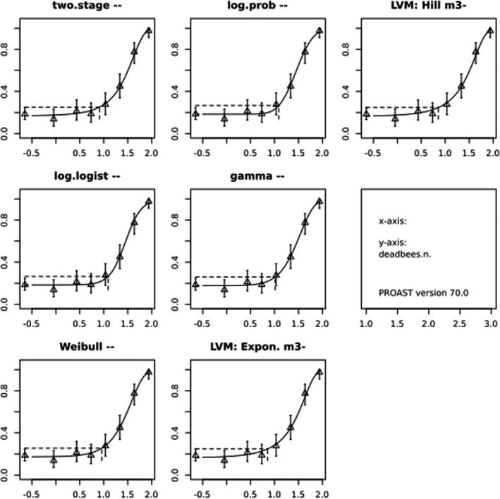
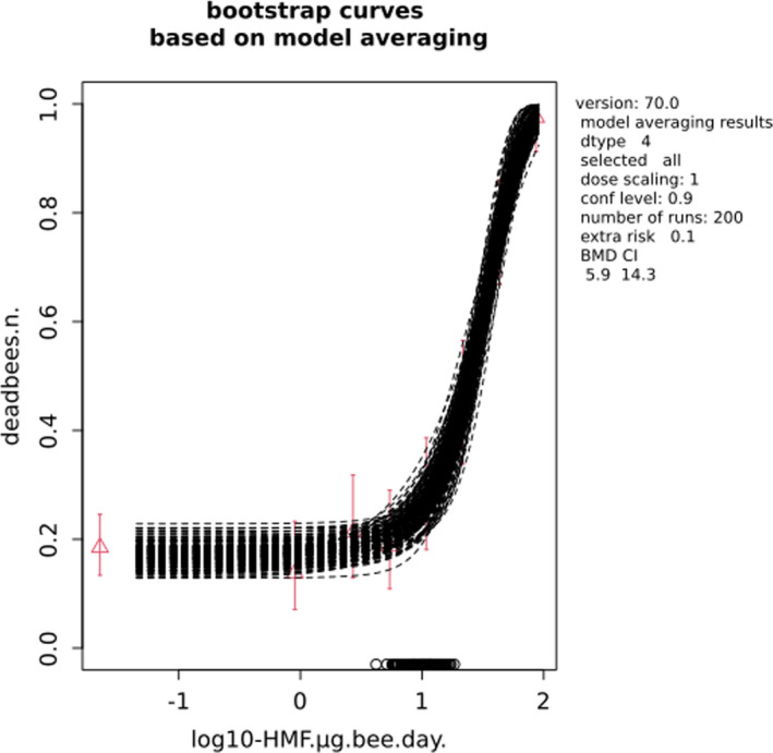
Appendix B – Additional information time reinforced toxicity assessment

B.1. Short introduction of the GUTS framework

The General Unified Threshold models of Survival (GUTS) framework was introduced to provide a common framework for a number of structurally different TKTD (toxicokinetic‐toxicodynamic) models for the description of the survival of individuals during exposure to chemicals (Jager et al., 2011). The framework assumes the uptake of a chemical into an organism (TK), translating external exposure into a so‐called 'dose metric’, and subsequent TD processes, which basically assume death to happen after an internal damage state has exceeded a certain threshold level. As ‘extreme cases’ of the GUTS framework, the individual tolerance (IT) and the stochastic death (SD) models were introduced, the IT model assuming individual internal threshold values, i.e. within a cohort of individuals a distribution of threshold values is found, and once an individual threshold value is exceeded, immediate death follows. The SD model in contrast assumes one constant threshold value for all individuals, but death happing with a certain so called 'killing rate constant’ as a random process.

In 2018, in the scientific opinion on TKTD models for aquatic risk assessment (EFSA PPR Panel, 2018), the GUTS framework was thoroughly evaluated and found to be ‘fit‐for‐purpose' for application in regulatory risk assessment, including the so‐called 'reduced GUTS’ (GUTS‐RED), which is using a simplified TK description that can also be calibrated without measured internal concentrations of chemicals. The terminology of the original GUTS framework was slightly changed (Jager and Ashauer, 2018), but GUTS is today frequently used in research and regulatory decision‐making.

B.2. Approach to determine the TRT property from survival data

The TRT property can be tested by applying regression modelling to observations on effective doses or concentrations observed over time. Experimental observations from toxicity tests cover, e.g. typically 10 days, and raw data (observations over time) from such tests can be used to estimate the slope factor as described above. However, a number of challenges come with such experimental approach: First, TRT considers only longer timescales, i.e. TRT might be clearly observable only for an exposure period of more than 10 days. However, if experiments are prolonged, often the control mortality (without exposure) is increasing over time, hampering a clear identification of the share of toxic effect in the overall observed mortality. Additionally, experimental data might appear with considerable variation in such log–log plots, which can lead to an uncertain identification of TRT in the regression step.

Therefore, for survival data, it is suggested that the TRT property of a chemical can be determined by using a modelling approach based on the GUTS framework (Jager et al., 2011; Jager and Ashauer, 2018; EFSA PPR Panel, 2018). The advantages of such GUTS‐based TRT derivation are threefold:

1. In case of long observation times which lead to increasing mortality over time, a modified reduced GUTS model including a two‐parameter background mortality model (see below) can be used to separate the background and chemically induced mortality.

2. In case of observations over shorter periods of time (e.g. 10 days) only, a calibrated GUTS model can be used to extrapolate mortality to longer exposure time periods.

3. By using all observed data point to calibrate a model with five parameters, the GUTS modelling is much more robust towards variability in the experimental observations and hence reduces uncertainty in the TRT determination.

The GUTS‐based derivation of the TRT property for a certain chemical then follows these four steps:

1. Calibration of a modified GUTS‐RED model.

2. Use of the calibrated GUTS‐RED model to create extrapolated time series of mortality for a wide range of exposure levels.

3. Fitting a dose‐response model to the GUTS‐derived, extrapolated time series of mortality and extraction of typical ecotoxicological values, e.g. lethal concentration (LC), for any choice of time points.

4. Application of the log–log regression model (equation 2), determination of the exponent b and finally assessment of the TRT property.

B.3. Assessment of TRT from critical studies

The assessment was performed separately using data from Gregorc et al. (2020) and Jachimowicz and El Sherbiny (1975).

In step 1, a modified GUTS‐RED‐SD model was used where everything was standard (Jager and Ashauer, 2018; EFSA PPR Panel, 2018), except the model for the control mortality. Only the SD model was used since it turned out in preparatory analyses that the IT model was not able to capture the TRT characteristic. In addition to the standard GUTS‐RED‐SD model, instead of using the simple exponential decline of survival without exposure for modelling background mortality in the equation for the survival probability

$$\mathrm{S}(\mathrm{t})={\mathrm{e}}^{-{\mathrm{h}}_{\mathrm{B}}·\mathrm{t}}·{\mathrm{e}}^{-\mathrm{H}\mathrm{a}\mathrm{z}(\mathrm{t})},$$ (B1)

with h_B being the background mortality rate, we used the cumulative distribution function of the log‐Normal distribution as two‐parameter background mortality model:

$$\mathrm{S}(\mathrm{t})=\left(1-\frac{1}{2}\mathrm{E}\mathrm{r}\mathrm{f}\mathrm{c}\left(\frac{{\mathrm{p}}_1-\mathrm{t}}{\sqrt{2}{\mathrm{p}}_2}\right)\right)·{\mathrm{e}}^{-\mathrm{H}\mathrm{a}\mathrm{z}(\mathrm{t})}.$$ (B2)

The parameters of the probability distribution function, p1 and p2, were fitted to the distribution of the observed life durations of the tested bees by minimisation of the negative log‐likelihood value based on the control survival data over time (see EFSA PPR Panel, 2018). If bees survived until the end of the experiments, censored data were used for the fitting.

The remaining three parameters of the GUTS‐SD‐RED model, the dominant rate constant k_D, the killing rate b and the internal threshold z, that jointly determine Haz in equation B2, were fitted to the survival over time by minimisation of the negative log‐likelihood function value by using the Simulated Annealing algorithm in the Method NMinimize in Mathematica 12.0. The fitted GUTS model is shown in Figures B.1 and B.2.

Figure B.1.

Fit of the modified GUTS model to the data from Gregorc et al. (2020); (left) survival in the control (C), and (right) four exposure levels (T1 = 100 mg, T2 = 500 mg, T3 = 1,000 mg and T4 = 1,500 mg). In the control, the parameters of the cumulative distribution function of the log‐normal distribution (see equation B1) were fitted to p1 = 3.2838 and p2 = 0.2772. For the whole data set, a log‐likelihood value of 5,881.54 was obtained for the best fit, and parameter values have been determined to k_D = 3.15·10⁻⁴; b = 3.81·10⁻³; z = 2.71·10⁻⁶


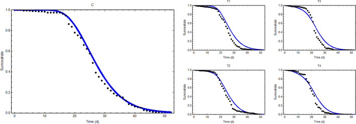
• d: day.

Figure B.2.

Fit of the modified GUTS model to the data from Jachimowicz and El Sherbiny (1975); survival in the control (C), and 3 exposure levels (T1 = 30 mg, T2 = 150 mg, T3 = 750 mg). Square symbols depict the ‘1973’ data series, diamonds the ‘1974’ data series. In the control, the parameters of the cumulative distribution function of the log‐normal distribution (see equation B1) were fitted to p1 = 36.1367, p2 = 16.2998. For the whole data set, a log‐likelihood value of 3500.002 was obtained for the best fit, and parameter values have been determined to k_D = 5.38·10⁻³, b = 23.60·10⁻³, z = 4.17·10⁻⁹⁴


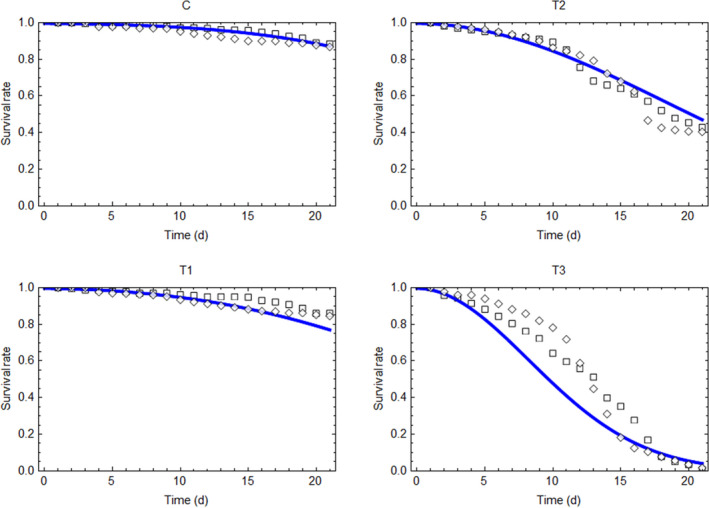
• d: day.

In step 2, for each data set, the calibrated GUTS was used to calculate survival for a series of 36 exposure levels between 10 and 10⁷ mg and exposure durations of 2, 3, 5, 7, 10, 15, 20, 30, 40, 50, 60, 70, 80, 90, 100, 150 and 180 days to cover different (and maximum) lifespans of winter bees. Background mortality was not considered for these extrapolations, only the toxic effect.

In step 3, the log‐logistic dose‐response function was fitted to the time series data as extrapolated by using the calibrated GUTS model (step 2). This is illustrated in Figure B.3. As described in the main text, LC₅₀ and LC₁₀ values were extracted for all considered exposure durations (Table 4, main Opinion).

Figure B.3.

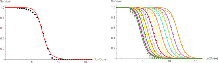
Survival data for different exposure durations and doses as extrapolated by the calibrated GUTS model (symbols), and corresponding fits of the log‐logistic dose‐response model (lines) based on data from Gregorc et al. (2020). (left) Example for an exposure duration of 30 days. (right) All dose response curves and simulated data points

Finally, in step 4, linear regressions of the logarithm of the LC₅₀ and LC₁₀ values, respectively, and the (simulated) duration of exposures was performed as described in the main Opinion and illustrated in Figures 5 and 6.

From fitting the GUTS model parameters, it appears that for both data sets, HMF shows what is called ‘slow kinetics’ according to Jager and Ashauer (2018): Small dominant rate constants, and in combination low internal threshold values. Based on observations of survival only, without having internal concentration measurements, it is not possible to say whether the slow kinetics is related to slow uptake of a compound, or to slow accrual of internal damage that is leading to mortality.

Annex A – Outcome of the public consultation on the draft opinion on the evaluation of the risks for animal health related to the presence of hydroxymethylfurfural (HMF) in feed for honey bees

Annex A is provided as a separate pdf file contain the outcome of the public consultation of the draft scientific Opinion, including the comments received and how they were taken into account when finalising the scientific Opinion.

Annex B – Raw data on occurrence of HMF in bee feed

The Annex B is provided as a separate Excel file available on the EFSA Knowledge Junction community on Zenodo at: https://doi.org/10.5281/zenodo.6406355

Supporting information

Outcome of the public consultation on the draft opinion on the evaluation of the risks for animal health related to the presence of hydroxymethylfurfural (HMF) in feed for honey bees

Suggested citation: EFSA CONTAM Panel (EFSA Panel on Contaminants in the Food Chain) , Bodin L, del Mazo J, Grasl‐Kraupp B, Hogstrand C, Leblanc J‐C, Bignami M, Hoogenboom L(R), Nebbia CS, Nielsen E, Ntzani E, Petersen A, Schrenk D, Vleminckx C, Wallace H, Focks A, Gregorc A, Metzler M, Sgolastra F, Tosi S, Horvath Zs, Ippolito A, Rortais A, Steinkellner H, Szentes C and Sand S, 2022. Scientific Opinion on the evaluation of the risks for animal health related to the presence of hydroxymethylfurfural (HMF) in feed for honey bees. EFSA Journal 2022;20(4):7227, 101 pp. 10.2903/j.efsa.2022.7227

References

- Abraham K, Gürtler R, Berg K, Heinemeyer G, Lampen A and Appel KE, 2011. Toxicology and risk assessment of 5‐hydroxymethylfurfural in food. Molecular Nutrition and Food Research, 55, 667–678. [DOI] [PubMed] [Google Scholar]
- ALjahdali N and Carbonero F, 2019. Impact of Maillard reaction products on nutrition and health: current knowledge and need to understand their fate in the human digestive system. Critical Reviews in Food Science and Nutrition, 59, 474–487. 10.1080/10408398.2017.1378865 [DOI] [PubMed] [Google Scholar]
- Aupinel P, Fortini D, Dufour H, Tasei JN, Michaud B, Odoux JF and Pham‐Delègue MH, 2005. Improvement of articial feeding in a standard in vitro method for rearing Apis mellifera larvae. Bulletin of Insectology, 58, 107–111. [Google Scholar]
- Bailey L, 1966. The effect of acid‐hydrolysed sucrose on honeybees. Journal of Apicultural Research, 5, 127–136. 10.1080/00218839.1966.11100146 [DOI] [Google Scholar]
- Ball DW, 2007. The chemical composition of honey. Journal of Chemical Education, 84, 1643–1646. [Google Scholar]
- Barker RJ and Lehner Y, 1974. Acceptance and sustenance value of naturally occurring sugars fed to newly emerged adult workers of honey bees (Apis mellifera L.). Journal of Experimental Zoology, 187, 277–285. [DOI] [PubMed] [Google Scholar]
- Berenbaum MR and Johnson RM, 2015. Xenobiotic detoxification pathways in honey bees. Current Opinion in Insect Science, 10, 51–58. [DOI] [PubMed] [Google Scholar]
- Bogdanov S, 2009. Harmonized methods of the International Honey Commission. Available online: https:www.ihc‐platform.net/ihcmethods2009.pdf/
- Bogdanov S, Lullmann C, Martin P, von der Ohe W, Russmann H, Vorwohl G, Oddo LP, Sabatini AG, Marcazzan GL, Piro R, Flamini C, Morlot M, Lheritier J, Borneck R, Panagyotis M, Tsigouri A, Kerkvliet J, Ortiz A, Ivanov T, D’Arcy B, Mossel B and Vit P, 1999. Honey quality and international regulatory standards: review by the International Honey Commission. Bee World, 80, 61–69. [Google Scholar]
- Böhme F, Bischoff G, Zebitz CPW, Rosenkranz P and Wallner K, 2018. From field to food ‐ will pesticide‐contaminated pollen diet lead to a contamination of royal jelly? Apidologie, 49, 112–119. 10.1007/s13592-017-0533-3 [DOI] [Google Scholar]
- Brodschneider R and Crailsheim K, 2010. Nutrition and health in honey bees. Apidologie, 41, 278–294. [Google Scholar]
- Capuano E and Fogliano V, 2011. Acrylamide and 5‐hydroxymethylfurfural (HMF) ‐ a review on metabolism, toxicity, occurrence in food and mitigation strategies. LWT –Food. Science and Technology, 44, 793–810. [Google Scholar]
- Ceksteryte V and Racys J, 2006. The quality of syrups used for bee feeding before winter and their suitability for bee wintering. Journal of Agricultural Science, 50, 5–14. [Google Scholar]
- Chen W, Wu S, Zhang J, Yu F, Miao X and Tu X, 2019. Salting‐out‐assisted liquid‐liquid extraction of 5‐hydroxymethylfurfural from honey and the determination of 5‐hydroxymethylfurfural by high‐performance liquid chromatography. Analytical Methods, 11, 4835–4841. [Google Scholar]
- Council of the EU (European Union) , 2021. Farming ministers reaffirm need for a new approach to protecting honey bees. Press release, 28 June 2021. Available online: https://www.consilium.europa.eu/en/press/press‐releases/2021/06/28/farming‐ministers‐reaffirm‐need‐for‐a‐new‐approach‐to‐protecting‐honey‐bees/
- Düll G, 1895. Über die Einwirkung von Oxalsäure auf Inulin. Chemiker‐Zeitung, 19, 216–217. [Google Scholar]
- EFSA (European Food Safety Authority) , 2010. Standard sample description for food and feed. EFSA Journal 2010;8(1):1457, 54 pp. 10.2903/j.efsa.2010.1457. Available online: www.efsa.europa.eu [DOI] [Google Scholar]
- EFSA (European Food Safety Authority) , 2011. Use of the EFSA Comprehensive European Food Consumption Database in Intakes Assessment. EFSA Journal 2011;9(3):2097, 34 pp. 10.2903/j.efsa.2011.2097 [DOI] [Google Scholar]
- EFSA (European Food Safety Authority) , 2013a. Standard Sample Description ver. 2.0. EFSA Journal 2013;11(10):3424, 114 pp. 10.2903/j.efsa.2013.3424 [DOI] [Google Scholar]
- EFSA (European Food Safety Authority) , 2013b. Guidance Document on the risk assessment of plant protection products on bees (Apis mellifera, Bombus spp. and solitary bees). EFSA Journal 2013;11(7):3295, 268 pp. 10.2903/j.efsa.2013.3295 [DOI] [PMC free article] [PubMed] [Google Scholar]
- EFSA (European Food Safety Authority) , Ippolito A, del Aguila M, Aiassa E, Muñoz Guajardo I, Neri FM, Alvarez F, Mosbach‐Schulz O and Szentes C, 2020. Review of the evidence on bee background mortality. EFSA supporting publication 2020;EN‐1880, 75 pp. 10.2903/sp.efsa.2020.EN-1880 [DOI]
- EFSA PPR Panel (EFSA Panel on Plant Protection Products and their Residues) , 2012. Scientific Opinion on the science behind the development of a risk assessment of Plant Protection Products on bees (Apis mellifera, Bombus spp. and solitary bees). EFSA Journal 2012;10(5):2668, 275 pp. 10.2903/j.efsa.2012.2668. Available online: https://www.efsa.europa.eu/en/efsajournal/pub/2668 [DOI] [Google Scholar]
- EFSA PPR Panel (EFSA Panel on Plant Protection Products and their Residues) , Ockleford C, Adriaanse P, Berny P, Brock T, Duquesne S, Grilli S, Hernandez‐Jerez AF, Bennekou SH, Klein M, Kuhl T, Laskowski R, Machera K, Pelkonen O, Pieper S, Smith RH, Stemmer M, Sundh I, Tiktak A, Topping CJ, Wolterink G, Cedergreen N, Charles S, Focks A, Reed M, Arena M, Ippolito A, Byers H and Teodorovic I, 2018. Scientific Opinion on the state of the art of Toxicokinetic/Toxicodynamic (TKTD) effect models for regulatory risk assessment of pesticides for aquatic organisms. EFSA Journal 2018;16(8):5377, 188 pp. 10.2903/j.efsa.2018.5377 [DOI] [PMC free article] [PubMed] [Google Scholar]
- EFSA Scientific Committee, Hardy A, Benford D, Halldorsson T, Jeger MJ, Knutsen KH, More S, Mortensen A, Naegeli H, Noteborn H, Ockleford C, Ricci A, Rychen G, Silano V, Solecki R, Turck D, Aerts M, Bodin L, Davis A, Edler L, Gundert‐Remy U, Sand S, Slob W, Bottex B, Abrahantes JC, Marques DC, Kass G and Schlatter JR, 2017. Update: Guidance on the use of the benchmark dose approach in risk assessment. EFSA Journal 2017;15(1):4658, 41 pp. 10.2903/j.efsa.2017.4658 [DOI] [PMC free article] [PubMed] [Google Scholar]
- EFSA Scientific Committee , Benford D, Halldorsson T, Jeger MJ, Knutsen HK, More S, Naegeli H, Noteborn H, Ockleford C, Ricci A, Rychen G, Schlatter JR, Silano V, Solecki R, Turck D, Younes M, Craig P, Hart A, Von Goetz N, Koutsoumanis K, Mortensen A, Ossendorp B, Martino L, Merten C, Mosbach‐Schulz O and Hardy A, 2018. Guidance on Uncertainty Analysis in Scientific Assessments. EFSA Journal 2018;16(1):5123, 39 pp. 10.2903/j.efsa.2018.5123 [DOI] [PMC free article] [PubMed] [Google Scholar]
- Farag MR, Alagawany M, Bin‐Jumah M, Othman SI, Khafaga AF, Shaheen HM, Samak D, Shehata AM, Allam AA and Abd El‐Hack ME, 2020. The toxicological aspects of the heat‐borne toxicant 5‐hyfroxymethylfurfural in animals: a review. Molecules, 25, 1941. [DOI] [PMC free article] [PubMed] [Google Scholar]
- Frizzera D, Del Fabbro S, Ortis G, Zanni V, Bortolomeazzi R, Nazzi F and Desiderato A, 2020. Possible side effects of sugar supplementary nutrition on honey bee health. Apidologie, 51, 594–608. 10.1007/s13592-020-00745-6 [DOI] [Google Scholar]
- Godfrey VB, Chen LJ, Griffin RJ, Lebetkin EH and Burka LT, 1999. Distribution and metabolism of (5‐hydroxymethyl)furfural in male F344 rats and B6C3F1 mice after oral administration. Journal of Toxicology and Environmental Health, Part A, 57, 199–210. [DOI] [PubMed] [Google Scholar]
- Gregorc A, Jurišić S and Sampson B, 2020. Hydroxymethylfurfural Affects Caged Honey Bees (Apis mellifera carnica). Diversity, 12, 18. 10.3390/d12010018 [DOI] [Google Scholar]
- Huang Z, 2018. Feeding honey bees. Extension Bulletin E‐3369. Michigan State University. Available online: https://pollinators.msu.edu/sites/_pollinators/assets/File/FeedingHoneyBees‐Final.pdf
- Jachimowicz T and El Sherbiny G, 1975. Zur problematik der verwendung von invertzucker für die bienenfütterung. Apidologie, 6, 121–143. 10.1051/apido:19750203 [DOI] [Google Scholar]
- Jager T, Albert C, Preuss TG and Ashauer R, 2011. General Unified Threshold model of Survival ‐ a toxicokinetic‐toxicodynamic framework for ecotoxicology. Environmental Science and Technology, 45, 2529–2540. [DOI] [PubMed] [Google Scholar]
- Jager T and Ashauer R, 2018. Modelling survival under chemical stress. A comprehensive guide to the GUTS framework. Version 2.0. Toxicodynamics Ltd., York, UK. Available online Leanpub: https://leanpub.com/guts_book
- Jalali S and Wohlin C, 2012. Systematic literature studies: database searches vs. backward snowballing. 6th ACM‐ IEEE International Symposium on Empirical Software Engineering and Measurement Lund. Available online: https://www.diva‐portal.org/smash/get/diva2:834640/FULLTEXT01.pdf [Google Scholar]
- Jeuring HJ and Kuppers FJ, 1980. High performance liquid chromatography of furfural and hydroxymethylfurfural in spirits and honey. Journal of the Association of Official Analytical Chemists, 63, 1215–1218. [PubMed] [Google Scholar]
- Johnson RM and Percel EG, 2013. Effect of a fungicide and spray adjuvant on queen‐rearing success in honey bees (Hymenoptera: Apidae). Journal of Economic Entomology, 106, 1952–1957. 10.1603/ec13199 [DOI] [PubMed] [Google Scholar]
- Kamboj R, Sandhu RS, Kaler RSS, Bera MB and Nanda V, 2019. Optimization of process parameters on hydroxynethylfurfural content, diastase and invertase activity of coriander honey. Journal of Food Science and Technology, 56, 3205–3214. [DOI] [PMC free article] [PubMed] [Google Scholar]
- Karabournioti S and Zervalaki P, 2001. The effect of heating on honey HMF and invertase. Apiacta, 36, 177–181. [Google Scholar]
- Kozianowski G, 2016. 5‐Hydroxymethylfurfural in bee feed (in German). Sugar Industry, 141, 575–583. [Google Scholar]
- Krainer S, Brodschneider R, Vollmann J, Crailsheim K and Riessberger‐Galle K, 2016. Effect of hydroxymethylfurfural (HMF) on mortality of artificially reared honey bee larvae (Apis mellifera carnica). Ecotoxicology, 25, 320–328. 10.1007/s10646-015-1590-x [DOI] [PubMed] [Google Scholar]
- LeBlanc BW, Eggleston G, Sammataro D, Cornett C, Dufault R, Deeby T and Cyr ES, 2009. Formation of hydroxymethylfurfural in domestic high‐fructose corn syrup and its toxicity to the honey bee (Apis mellifera). Journal of Agricultural and Food Chemistry, 57, 7369–7376. [DOI] [PubMed] [Google Scholar]
- Lüken DJ and von der Ohe W, 2016. Aufklärung der Wirkung des Gehaltes an Hydroxymethylfurfural (HMF) in Futtermitteln für Bienen hinsichtlich der Tiergesundheit und des Carry overs von HMF in Honig (Evaluation of the effect of the HMF level in bee feed on animal health and on the transfer of HMF in honey). Schlussbericht zum Forschungsauftrag, BLE Projektträger‐Datenbank, Projektnummer 314‐06.01‐2815HS002 (Final report on the research assignment, project sponsor database of the Federal Office for Agriculture and Food, project number 314‐06.01‐2815HS002). Available online: https://service.ble.de/ptdb/index2.php?detail_id=57202&site_key=145&zeilenzahl_zaehler=589&NextRow=40&pId=57202&dId=321065
- Maillard LC, 1912. Action des acides aminés sur les sucres; formation des mélanoidines par voie methodique. Comptes Rendus De L'académie Des Sciences, 154, 66–68. [Google Scholar]
- Morales FJ, 2009. Hydroxymethylfurfural (HMF) and related compounds. In: Stadler RH and Lineback DR (eds.)., Process‐Induced food toxicants: Occurrence, formation, mitigation and health risks, John Wiley & Sons Inc, New York. pp. 134–175. [Google Scholar]
- Mulvey J and Cresswell JE, 2020. Time‐dependent effects on bumble bees of dietary exposures to farmland insecticides (imidacloprid, thiamethoxam and fipronil). Pest Management Science, 76, 2846–2853. 10.1002/ps.5838 [DOI] [PubMed] [Google Scholar]
- NFI‐DTU (National Food Institute, Technical University of Denmark) , Bredsdorff L, Olesen PL, Sharma AK, Hansen M, Jørgensen K, Ekstrøm J, Ravn‐Haren G, Skjolding LM, Baun A and Beltoft VM, 2020. Extensive literature search on grayanotoxins and 5‐hydroxymethylfurfural. EFSA supporting publication 2020;EN‐1920, 52 pp. 10.2903/sp.efsa.2020.EN-1920 [DOI]
- OECD (Organisation for Economic Co‐operation and Development) , 2016. Guidance document on honey bee larval toxicity text following repeated exposure. Series on Testing and Assessment No. 239. Available online: https://www.oecd.org/officialdocuments/publicdisplaydocumentpdf/?cote=env/jm/mono(2016)34&doclanguage=en
- OECD (Organisation for Economic Co‐operation and Development) , 2017. Test No. 245: Honey Bee (Apis Mellifera L.), Chronic Oral Toxicity Test (10‐Day Feeding), OECD Guidelines for the Testing of Chemicals, Section 2, OECD Publishing, Paris. 10.1787/9789264284081-en [DOI]
- Pryor RL, Wu X and Gu L, 2006. Identification of urinary excretion of metabolites of 5‐(hydroxymethyl)‐2‐furfural in human subjects following consumption of dried plums or dried plum juice. Journal of Agriculture and Food Chemistry, 54, 3744–3749. [DOI] [PubMed] [Google Scholar]
- Remolina SC and Hughes KA, 2008. Evolution and mechanisms of long life and high fertility in queen honey bees. Age (Dordr), 30, 177–185. [DOI] [PMC free article] [PubMed] [Google Scholar]
- Rortais A, Arnold G, Halm M‐P and Touffet‐Briens F, 2005. Modes of honeybee exposure to systemic insecticides: estimated amounts of contaminated pollen and nectar consumed by different categories of bees. Apidologie, 36, 71–83. 10.1051/apido:2004071 [DOI] [Google Scholar]
- Ruiz‐Matute AI, Weiss M, Sammataro D, Finely J and Sanz ML, 2010. Carbohydrate composition of high‐fructose corn syrups used for bee feeding: effect on honey composition. Journal of Agricultural and Food Chemistry, 58, 7317–7322. [DOI] [PubMed] [Google Scholar]
- Semkiw P and Skubida P, 2016. Suitability of starch syrups for winter feeding of honey bee colonies. Journal of Apicultural Science, 60, 141–152. 10.1515/jas-2016-0025 [DOI] [Google Scholar]
- Shapla UM, Solayman M, Alam N, Khalil MI and Gan SH, 2018. 5‐Hydroxymethylfurfural (HMF) levels in honey and other food products: effects on bee and human health. Chemistry Central Journal, 12, 35. [DOI] [PMC free article] [PubMed] [Google Scholar]
- Simpson J, Riedel IB and Wilding N, 1968. Invertase in the hypopharyngeal glands of the honeybee. Journal of Apicultural Research, 7, 29–36. [Google Scholar]
- Smodiš Škerl MI and Gregorc A, 2014. A preliminary laboratory study on the longevity of A. m. carnica honey bees after feeding with candies containing HMF. Google Scholar. Journal of Apicultural Research, 53, 422–423. 10.3896/IBRA.1.53.4.07 [DOI] [Google Scholar]
- Somerville D, 2014. Feeding sugars to honey bees. Primefact 1343, NSW Department of Primary Industries. Feeding sugar to honey bees (nsw.gov.au).
- Tennekes H, 2010. The significance of the Druckrey‐Küpfmüller equation for risk assessment ‐ the toxicity of neonicotinoid insecticides to arthropods is reinforced by exposure time. Toxicology, 276, 1–4. [DOI] [PubMed] [Google Scholar]
- Tosi E, Ciappini M, Re E and Lucero H, 2001. Honey thermal treatment effects on hydroxymethylfurfural content. Food Chemistry, 77, 71–74. [Google Scholar]
- Tosi S, Nieh JC, Brandt A, Colli M, Fourrier J, Giffard H, Hernández‐lópez J, Malagnini V, Williams GR and Simon‐delso N, 2021. Long‐term field‐realistic exposure to a next‐generation pesticide, flupyradifurone, impairs honey bee behaviour and survival. Communications Biology, 4 pp. 1–9. 10.1038/s42003-021-02336-2 [DOI] [PMC free article] [PubMed] [Google Scholar]
- Truzzi C, Annibaldi A, Illuminati S, Finale C, Rossetti M and Scarponi G, 2012. Determination of very low levels of 5‐(hydroxymethyl)‐2‐furaldehyde (HMF) in natural honey: comparison between the HPLC technique and the spectroscopic White method. Journal of Food Science, 77, C784–C790. [DOI] [PubMed] [Google Scholar]
- Van der Zee R and Pisa LB, 2010. 2009–10 en toxische invertsuikersiroop. NCB Rapporten, 2, 1–15. [Google Scholar]
- Van der Zee R and Pisa LB, 2011. 2009–10 en toxische invertsuikersiroop. NCB Rapporten 1. [Google Scholar]
- White JW, 1979. Spectrophotometric method for hydroxymethylfurfural in honey. Journal of the Association of Official Analytical Chemists, 62, 509–514. [PubMed] [Google Scholar]
- Wilmart O, Reybroeck W, De Meulenaer B, de Graaf DC, Nguyen BK, Huyghebaert A and Saegerman C, 2011. Analyse du risque poséen santéanimale par la présence de l’hydroxyméthylfurfural dans lessirops de nourrissement des abeilles domestiques. Annales De Médecine Vétérinaire, 155, 53–60. [Google Scholar]
- Winkler O, 1955. Beitrag zum Nachweis und zur Bestimmung von Oxymethylfurfurol in Honig und Kunsthonig. Zeitschrift Für Lebensmittel‐Untersuchung Und ‐Forschung, 102, 161–167. [Google Scholar]
- Yang W, Zhang C, Li C, Huang ZY and Miao X, 2019. Pathway of 5‐hydroxymethyl‐2‐furaldehyde formation in honey. Journal of Food Science and Technology, 56, 2417–2425. [DOI] [PMC free article] [PubMed] [Google Scholar]
- Zappalà M, Fallico B, Arena E and Verzera A, 2005. Methods for the determination of HMF in honey: a comparison. Food Control, 16, 273–277. [Google Scholar]
Associated Data
This section collects any data citations, data availability statements, or supplementary materials included in this article.
Supplementary Materials