Optimal control problem arising from COVID-19 transmission model with rapid-test

Abstract

The world health organization (WHO) has declared the Coronavirus (COVID-19) a pandemic. In light of this ongoing global issue, different health and safety measure has been recommended by the WHO to ensure the proactive, comprehensive, and coordinated steps to bring back the whole world into a normal situation. This is an infectious disease and can be modeled as a system of non-linear differential equations with reaction rates which consider the rapid-test as the intervention program. Therefore, we have developed the biologically feasible region, i.e., positively invariant for the model and boundedness solution of the system. Our system becomes well-posed mathematically and epidemiologically for sensitive analysis and our analytical result shows an occurrence of a forward bifurcation when the basic reproduction number is equal to unity. Further, the local sensitivities for each model state concerning the model parameters are computed using three different techniques: non-normalizations, half-normalizations, and full normalizations. The numerical approximations have been measured by using System Biology Toolbox (SBedit) with MATLAB, and the model is analyzed graphically. Our result on the sensitivity analysis shows a potential of rapid-test for the eradication program of COVID-19. Therefore, we continue our result by reconstructing our model as an optimal control problem. Our numerical simulation shows a time-dependent rapid test intervention succeeded in suppressing the spread of COVID-19 effectively with a low cost of the intervention. Finally, we forecast three COVID-19 incidence data from China, Italy, and Pakistan. Our result suggests that Italy already shows a decreasing trend of cases, while Pakistan is getting closer to the peak of COVID-19.

Introduction

It is likely that this infectious disease (COVID-19) originated in an animal species, and then spread to humans. Person to person spread of the novel coronavirus reported daily throughout the world. This virus involves serious respiratory tract infections [1], [2]. Therefore, all the countries are making all-out efforts to deal with a rapidly evolving situation which is a challenge for the whole world. An emergency has been declared in infected areas of the world and a serious public health concern has been paid at a global level. Now, it is important to understand how to get control by monitoring the spreading of this disease. Within this urgency, doctors and paramedical staff are on the front line for treating the COVID-19 patients. While to stop the impact of this infection and to avoid further spreading some mathematical estimations are also being performed at each level. Some method has been proposed by the researches based on the mathematical modeling for calculating the basic reproduction number [3], [4].

Various ways have been conducted by the government all over the world to suppress the spread of COVID-19 on their countries, such as with social distancing, international travel restrictions, rapid-test, and even lockdown [5]. Many mathematical models conclude that lockdown is the best way to reduce the spread of COVID-19 effectively among all the aforementioned control strategies [6]. However, lockdown interventions are very risky for a country’s economic stability, Pakistan, India, Iran. Therefore, as a step to prevent the increasing number of infections, social distancing interventions to minimize the successful contact of infections and rapid-test to map the spread of infection into options in various countries [5], [7], instead of implementing lockdown in their countries. Computational results give an essential way to identify the key critical elements based on the modern decomposition techniques [8], [9], [10] in different available reaction routes [11], [12] that allow us to discuss the dynamical properties of the suggested models of the COVID-19. Recently, some models of the COVID-19 have suggested, they provide a good step forward to understand the dynamics of this disease [13], [14], [15], [16]. Accordingly, some suggested mathematical models were reviewed and some computational simulations investigated for the confirmed cases in China [17]. More recently, we developed an updated model of the COVID-19, we have also identified some key critical parameters with sensitivity analysis [18].

Although some mathematical models have been projected so far for new coronavirus disease prediction, a lot can still be improved. Defining such models based on mass action law with reaction rate constants and calculating the sensitivities for each model state with respect to model parameters could improve the outcomes. In a complicated modeling case like new coronavirus dynamics, it is necessary to pay more attention to the optimal control problem and sensitivity analysis more accurately and widely.

Here in this article, we further developed our previous model, some transmission paths and parameters are added. We focused on analyzing the effect of COVID-19 rapid-test as an alternative to suppress the spread of COVID-19. Another novelty of the paper is the identification of the critical model parameters, which makes it easy for the biologists to be used with less knowledge of mathematical modeling and also facilitates the improvement of the model for future development. Consequently, here we measure the effect of rapid-test infection identification on the COVID-19 free equilibrium point and the reproduction number for local stability. Interestingly, the optimal control problem applied to the established model shows that the time-dependent interventions which adapt to the number of infections are able to reduce the number of COVID-19 infections well and at a much lower cost. Finally, we give some short time forecasting of three countries (China, Italy and Pakistan) using our proposed model.

A mathematical model of COVID-19

Let assume the human population can be separated depending on their health status respected to infection status on COVID-19 disease, both visually (symptoms) or through a medical test. Next, let us consider that there is a random test to check whether someone is infected with COVID-19 or not. Then, we split the human class into 5 different classes.

• 1.Susceptible class ($S$): This class presents a healthy individual.
• 2.Asymptomatic class ($A$): This class presents an infected individual in the early stage of infection. They do not show any symptoms, but capable to infect through droplets or direct contact with the susceptible individual. Because they do not show any symptoms, these individuals are still easy to perform social contact with everyone since they do not realize that they are infected by COVID-19.
• 3.Symptomatic Unreported class ($U$): This class presents an individual who gets infected, had symptoms of COVID-19, but did not detect by the government as a COVID-19 suspect.
• 4.Symptomatic reported class ($I$): This class presents an individual who gets infected, shows a symptoms of COVID-19, and detected by the government, either it from a rapid test, or from voluntary action to report to the hospital. We assume that all individuals in this class will get a specific treatment and supervision, whether it is through monitored isolation or treatment in the hospital.
• 5.Recovered class ($R$): This class present individual who get recovered from COVID-19, and had a temporal immunity.

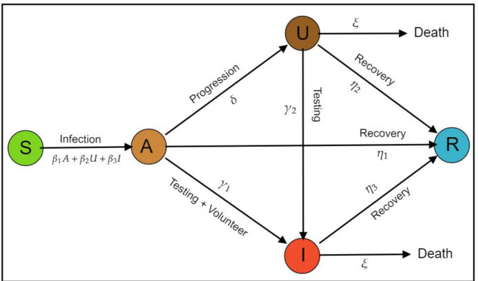
The transmission diagram which illustrates the interaction between each class described in Fig. 1.

Fig. 1.

Transmission diagram of COVID-19 with the effect of rapid-test.

The explanation about model construction is as follows. Susceptible individual increased caused by natural birth rate $\Lambda$, and infection from $A,U$ and $I$ with effective contact rate ${\beta }_1,{\beta }_2$ and ${\beta }_3$, respectively. Note that ${\beta }_2>{\beta }_1>{\beta }_3$ since undetected infected individuals still have full access to perform a contact social with randomly. On the other hand, $I$ has the smallest infection rate caused by an infected individual already detected by the government, which isolated in the hospital or monitored by the government to conduct self-isolation in their home. Individuals in $A$ increased cause by infection from $S$, and decreased caused by recovery to $R$ with a rate of ${\eta }_1$, progression in symptomatic to $U$ with a rate of $\delta$ and the infectious detected individual with the rate of ${\gamma }_1$. ${\gamma }_1$ present both human awareness to report their health status to the government about their symptoms, so they can get treatment by the government, or detected by rapid test intervention by the government. Please note that ${\gamma }_2>{\gamma }_1$ since we assume that the government has more concerned to bring the symptomatic individual into the hospital. Undetected symptomatic individual $U$ increased by progression from $A$ and decreased by recovery with constant rate ${\eta }_2$, rapid test ${\gamma }_2$ and death rate induced by COVID-19 $\xi$. Detected symptomatic infectious individual $I$ increased by progression from $A$, rapid test from $U$, and decreased by recovery rate ${\eta }_3$ and death rate induced by COVID-19. Last, recovered compartment $R$ increased by recovery rate from all infected individuals. Each compartment decreased by natural death rate $\mu$.

Based on the transmission diagram in Fig. 1 and aforementioned explanation, the model equation to describe the effect of rapid test in the spread of COVID-19 is as follows:

$$\begin{array}{c}\frac{dS}{dt}=\Lambda -S\left({\beta }_{1}A+{\beta }_{2}U+{\beta }_{3}I\right)-\mu S,\hfill \\ \frac{dA}{dt}=S\left({\beta }_{1}A+{\beta }_{2}U+{\beta }_{3}I\right)-\delta A-{\gamma }_{1}A-{\eta }_{1}A-\mu A,\hfill \\ \frac{dU}{dt}=\delta A-{\gamma }_{2}U-{\eta }_{2}U-\xi U-\mu U,\hfill \\ \frac{dI}{dt}={\gamma }_{1}A+{\gamma }_{2}U-{\eta }_{3}I-\xi I-\mu I,\hfill \\ \frac{dR}{dt}={\eta }_{1}A+{\eta }_{2}U+{\eta }_{3}I-\mu R.\hfill \end{array}$$ (1)

This model supplemented with the non-negative initial condition, and note that all parameters are positive.

Model analysis

Basic properties

Epidemiological meaningfulness of system (1) is one of the paramount analyzes in this section since it describes the human population. We perform the following theorem about the positiveness solution of the system (1).

Theorem 1

Let the initial conditions:

$$S\left(0\right)\ge 0,A\left(0\right)\ge 0,U\left(0\right)\ge 0,I\left(0\right)\ge 0,R\left(0\right)\ge 0$$

exist in the interval$t\in [0,\infty )$, then the solutions$S\left(t\right),A\left(t\right),U\left(t\right),I\left(t\right)$and$R\left(t\right)$of system (1) are positive for all $t\ge 0$ .

Proof

From system (1), we obtain:

$${\frac{dS}{dt}|}_{S=0,A\ge 0,U\ge 0,I\ge 0,R\ge 0}=\Lambda >0,$$

$${\frac{dA}{dt}|}_{S\ge 0,A=0,U\ge 0,I\ge 0,R\ge 0}=S\left({\beta }_{1}A+{\beta }_{2}U+{\beta }_{3}I\right)\ge 0,$$

$${\frac{dU}{dt}|}_{S\ge 0,A\ge 0,U=0,I\ge 0,R\ge 0}=\delta A\ge 0,$$

$${\frac{dI}{dt}|}_{S\ge 0,A\ge 0,U\ge 0,I=0,R\ge 0}={\gamma }_{1}A+{\gamma }_{2}U\ge 0,$$

$${\frac{dR}{dt}|}_{S\ge 0,A\ge 0,U\ge 0,I\ge 0,R=0}={\eta }_{1}A+{\eta }_{2}U+{\eta }_{3}I\ge 0.$$

The above rates are all non-negative over their boundary planes of the non-negative cone ${\mathbb{R}}_{+}^5$. Therefore, we have the direction of vector fields intended inward from their boundaries. Consequently, we are starting from the non-negative initial conditions so that all the solutions of the system (1) remains positive for all the time $t>0$. Hence, the following theorem implies the boundedness solution of the system (1).

Theorem 2

The biologically feasible region

$$\Omega =\left\{(S,A,U,I,R)\in {\mathbb{R}}_{+}^5:S+A+U+I+R\le \frac{\Lambda }{\mu }\right\}$$

is positively invariant for the model (1) .

Proof

Since

$$\frac{dN}{dt}=\frac{d(S+A+U+I+R)}{dt}=\Lambda -\mu N-\xi (U+I)\le \Lambda -\mu N,$$

we have that $N\left(t\right)\le N\left(0\right)e^{-\mu t}+\frac{\Lambda }{\mu }\left[1-e^{-\mu t}\right]$. Basically, $N\left(t\right)\le \frac{\Lambda }{\mu }$ with respect to the condition $N\left(0\right)\le \frac{\Lambda }{\mu }$. Therefore, we have that $\Omega$ to be positively invariant and attracting which suffices system (1) can be considered in $\Omega$. Hence, system (1) considered being well-posed mathematically and epidemiologically.

COVID-19 free equilibrium point and the reproduction number

The COVID-19 free equilibrium point of system (1) is given by:

$$E_1=\left(S_1,A_1,U_1,I_1,R_1\right)=\left(\frac{\Lambda }{\mu },0,0,0,0\right).$$ (2)

To analyze the local stability of $E_1$, first, we construct the valued basic reproduction number of system (1) using the next-generation matrix approach (Please see [19] for further detail, and more example in [20], [21], [22], [23], [24], [25]). The basic reproduction number of system (1) is given by:

$${\mathcal{R}}_0={\mathcal{R}}_{\text{asymptomatic}}+{\mathcal{R}}_{\text{undetected}}+{\mathcal{R}}_{\text{detected}},$$ (3)

where

$${\mathcal{R}}_{\text{asymptomatic}}=\frac{{\beta }_1\Lambda }{\mu (\delta +{\eta }_1+{\gamma }_1)},$$ (4)

$${\mathcal{R}}_{\text{undetected}}=\frac{{\beta }_2\Lambda \delta }{\mu (\delta +{\eta }_1+{\gamma }_1)(\xi +{\eta }_2+{\gamma }_2)},$$ (5)

$${\mathcal{R}}_{\text{detected}}=\frac{{\beta }_3\Lambda \left(\delta {\gamma }_2+\xi {\gamma }_1+{\eta }_2{\gamma }_1+{\gamma }_1{\gamma }_2\right)}{\mu (\delta +{\eta }_1+{\gamma }_1)(\xi +{\eta }_2+{\gamma }_2)(\xi +{\eta }_3)}.$$ (6)

Note that ${\mathcal{R}}_0$ is the summation of three types of “local” basic reproduction numbers depending on the origin of the infection, whether it from asymptomatic $\left({\mathcal{R}}_{\text{asymptomatic}}\right)$, undetected symptomatic $\left({\mathcal{R}}_{\text{undetected}}\right)$ or detected symptomatic $\left({\mathcal{R}}_{\text{detected}}\right)$ individuals.

Having the basic reproduction number in hand, and using [29], we have the following theorem regarding the local stability of $E_1$.

Theorem 3

The COVID-19 free equilibrium$E_1$of the system (1) is locally asymptotically stable if ${\mathcal{R}}_0<1$ , and unstable if ${\mathcal{R}}_0>1$ .

${\mathcal{R}}_0$ presents the expected number of secondary cases of COVID-19 which generated by a single infection introduced into a community of totally susceptible individuals. The results in Theorem 3 shows that COVID-19 can be eliminated in the community when the basic reproduction number is less than unity.

Endemic equilibrium point

The COVID-19 endemic equilibrium point of system (1) is given by

$$E_2=\left(S_2,A_2,U_2,I_2,R_2\right),$$ (7)

where

$$S_2=\frac{\Lambda \left(\delta {\gamma }_2+\mu {\gamma }_1+\xi {\gamma }_1+{\eta }_2{\gamma }_1+{\gamma }_1{\gamma }_2\right)}{K_1{I}_2+K_2}$$

$$A_2=\frac{{\mathit{I}}_{\mathit{2}}\left(\mu +\xi +{\eta }_3\right)\left(\mu +\xi +{\eta }_2+{\gamma }_2\right)}{\delta {\gamma }_2+\mu {\gamma }_1+\xi {\gamma }_1+{\eta }_2{\gamma }_1+{\gamma }_1{\gamma }_2},$$

$$U_2=\frac{{\mathit{I}}_{\mathit{2}}\delta \left(\mu +\xi +{\eta }_3\right)}{\delta {\gamma }_2+\mu {\gamma }_1+\xi {\gamma }_1+{\eta }_2{\gamma }_1+{\gamma }_1{\gamma }_2},$$

$$R_2=\frac{I_2{K}_3}{\mu \left(\delta {\gamma }_2+\mu {\gamma }_1+\xi {\gamma }_1+{\eta }_2{\gamma }_1+{\gamma }_1{\gamma }_2\right)},$$

and

$$K_1=\left(\mu +\xi +{\eta }_3\right)\left(\mu +\xi +{\eta }_2+{\gamma }_2\right){\beta }_1+\left(\delta {\beta }_2+{\beta }_3{\gamma }_1\right)\mu ,+\left(\delta {\beta }_2+{\beta }_3{\gamma }_1\right)\xi +{\beta }_3\left(\delta +{\gamma }_1\right){\gamma }_2+\delta {\beta }_2{\eta }_3+{\beta }_3{\eta }_2{\gamma }_1,$$

$$K_2=\mu \left(\delta {\gamma }_2+\mu {\gamma }_1+\xi {\gamma }_1+{\eta }_2{\gamma }_1+{\gamma }_1{\gamma }_2\right),$$

$$K_3=\left(\mu +\xi +{\eta }_3\right)\left(\mu +\xi +{\eta }_2+{\gamma }_2\right){\eta }_1+\left(\left(\delta +{\gamma }_1\right){\eta }_2+\mu {\gamma }_1+\xi {\gamma }_1+{\gamma }_2\left(\delta +{\gamma }_1\right)\right){\eta }_3+\delta {\eta }_2\left(\mu +\xi \right).$$

$I_2$ is taken from the positive root of linear equation given by:

$$K_{4}I-K_5\left({\mathcal{R}}_0-1\right)=0$$ (8)

where

$$K_4=\left(\mu +\xi +{\eta }_3\right)\left(\mu +\xi +{\eta }_2+{\gamma }_2\right)\left(\delta +\mu +{\eta }_1+{\gamma }_1\right)K_{41},$$

$$K_{41}=\left(\mu +\xi +{\eta }_3\right)\left(\mu +\xi +{\eta }_2+{\gamma }_2\right){\beta }_1,+\left(\delta {\beta }_2+{\beta }_3{\gamma }_1\right)\mu +\left(\delta {\beta }_2+{\beta }_3{\gamma }_1\right)\xi ,+{\beta }_3\left(\delta +{\gamma }_1\right){\gamma }_2+\delta {\beta }_2{\eta }_3+{\beta }_3{\eta }_2{\gamma }_1,$$

$$K_5=\left(\delta {\gamma }_2+\mu {\gamma }_1+\xi {\gamma }_1+{\eta }_2{\gamma }_1+{\gamma }_1{\gamma }_2\right)\mu \left(\mu +\xi +{\eta }_3\right)\left(\mu +\xi +{\eta }_2+{\gamma }_2\right)\left(\delta +\mu +{\eta }_1+{\gamma }_1\right).$$

It can be seen from (8) that $I_2$ will be positive if ${\mathcal{R}}_0>1$. The existence of the endemic equilibrium is given in the following theorem.

Theorem 4

The COVID-19 endemic equilibrium point$E_2$of the system (1) exist if condition ${\mathcal{R}}_0>1$ holds.

Bifurcation analysis

On the system (1), we assumed

$$S=x_1,A=x_2,U=x_3,I=x_4,R=x_5,$$

$$\frac{dS}{dt}=g_1,\frac{dA}{dt}=g_2,\frac{dU}{dt}=g_1,\frac{dI}{dt}=g_1,\frac{dR}{dt}=g_1.$$

Therefore, system (1) can be re-written as

$$g_1=\Lambda -x_1\left({\beta }_1{x}_2+{\beta }_2{x}_3+{\beta }_3{x}_4\right)-\mu x_1,$$$$g_2=x_1\left({\beta }_1{x}_2+{\beta }_2{x}_3+{\beta }_3{x}_4\right)-\delta x_2-{\gamma }_1{x}_2-{\eta }_1{x}_2-\mu x_2,$$$$g_3=\delta x_2-{\gamma }_2{x}_3-{\eta }_2{x}_3-\xi x_3-\mu x_3,$$$$g_4={\gamma }_1{x}_2+{\gamma }_2{x}_3-{\eta }_3{x}_4-\xi x_4-\mu x_4,$$$$g_5={\eta }_1{x}_2+{\eta }_2{x}_3+{\eta }_3{x}_4-\mu x_5.$$ (9)

Next, let ${\beta }_1$ as the bifurcation parameter. To do this, we solve ${\mathcal{R}}_0=1$ respect to ${\beta }_1$ to yield ${\beta }_1^{\ast }$ which is given by

$${\beta }_1^{\ast }=\frac{\mu (\delta +{\eta }_1+{\gamma }_1)}{\Lambda }\left({\mathcal{R}}_0-{\mathcal{R}}_{\text{undetected}}-{\mathcal{R}}_{\text{detected}}\right)$$

Next, substitute $E_1$ and ${\beta }_1^{\ast }$ to the Jacobian matrix of system (9) which will gave us:

$$J_{E_1,{\beta }_1={\beta }^{\ast }}=\left[\begin{array}{ccccc}\hfill -\mu \hfill & \hfill -\frac{\Lambda {\beta }^{\ast }}{\mu }\hfill & \hfill -\frac{\Lambda {\beta }_2}{\mu }\hfill & \hfill -\frac{\Lambda {\beta }_3}{\mu }\hfill & \hfill 0\hfill \\ \hfill 0\hfill & \hfill \frac{\Lambda {\beta }^{\ast }}{\mu }-\delta -\mu -{\eta }_1-{\gamma }_1\hfill & \hfill \frac{\Lambda {\beta }_2}{\mu }\hfill & \hfill \frac{\Lambda {\beta }_3}{\mu }\hfill & \hfill 0\hfill \\ \hfill 0\hfill & \hfill \delta \hfill & \hfill -\mu -\xi -{\eta }_2-{\gamma }_2\hfill & \hfill 0\hfill & \hfill 0\hfill \\ \hfill 0\hfill & \hfill {\gamma }_1\hfill & \hfill {\gamma }_2\hfill & \hfill -\mu -\xi -{\eta }_3\hfill & \hfill 0\hfill \\ \hfill 0\hfill & \hfill {\eta }_1\hfill & \hfill {\eta }_2\hfill & \hfill {\eta }_3\hfill & \hfill -\mu \hfill \end{array}\right].$$

This matrix has one simple zero eigenvalues, while the other four are negative. Therefore, we can use a center-manifold approach to analyze the stability of the endemic equilibrium when ${\mathcal{R}}_0$ close to one.

Firstly, we look for the right eigenvector and left eigenvector. Let vector $\overrightarrow{w}=(w_1,w_2,w_3,w_4,w_5)$ as the right eigenvector of simple zero eigenvalue of $J_{E_1,{\beta }_1={\beta }^{\ast }}$. The right eigenvector $\overrightarrow{w}$ is given by

$$w_1=-\frac{\left(\delta +{\eta }_1+{\gamma }_1+\mu \right)\left(\mu +\xi +{\eta }_2+{\gamma }_2\right)}{\delta \mu },$$$$w_2=\frac{\mu +\xi +{\eta }_2+{\gamma }_2}{\delta },$$$$w_3=1,$$$$w_4=\frac{\delta {\gamma }_2+{\gamma }_1\mu +\xi {\gamma }_1+{\eta }_2{\gamma }_1+{\gamma }_1{\gamma }_2}{\delta \left(\mu +\xi +{\eta }_3\right)},$$$$w_5=\frac{\left(\mu +\xi +{\eta }_3\right)\left(\mu +\xi +{\eta }_2+{\gamma }_2\right){\eta }_1+\left({\gamma }_1\mu +\xi {\gamma }_1+\left({\gamma }_2+{\eta }_2\right)\left({\gamma }_1+\delta \right)\right){\eta }_3+\delta {\eta }_2\left(\mu +\xi \right)}{\delta \left(\mu +\xi +{\eta }_3\right)\mu }$$ (10)

Similarly, let the left eigenvector of $J_{E_1,{\beta }_1={\beta }^{\ast }}$ is given by $\overrightarrow{v}=(v_1,v_2,v_3,v_4,v_5)$. Therefore, the left eigenvector $\overrightarrow{v}$ is obtained as follows:

$$v_1=0,$$$$v_2=\frac{v_4\left(\mu +\xi +{\eta }_3\right)\mu }{\Lambda {\beta }_3},$$$$v_3=\frac{\left(\mu {\beta }_2+\xi {\beta }_2+{\beta }_2{\eta }_3+{\beta }_3{\gamma }_2\right)v_4}{{\beta }_3\left(\mu +\xi +{\eta }_2+{\gamma }_2\right)},$$$$v_4=1,$$$$v_5=0.$$ (11)

Since the eigenvector $v_1=0$ and $v_5=0$, so there is no need to look for a partial derivative of $g_1$ and $g_5$. Therefore, we find the derivatives of $g_2$, $g_3$, and $g_4$ to get the values $\mathcal{A}$ and $\mathcal{B}$ in the Castillo-Song bifurcation theorem [30]. From non-zero $g_2$, $g_3$ and $g_4$, the derivatives are as follows:

$$\frac{{\partial }^2{g}_2}{\partial x_1\partial x_2}=\frac{{\partial }^2{g}_2}{\partial x_2\partial x_1}=\frac{1}{\Lambda \left(\mu +\xi +{\eta }_3\right)\left(\mu +\xi +{\eta }_2+{\gamma }_2\right)}\times \left(\left(\left(-\Lambda {\beta }_3+{\mu }^2+\mu \xi +\mu {\eta }_3\right){\gamma }_2+\left(\mu +\xi +{\eta }_3\right)\left(-\Lambda {\beta }_2+{\mu }^2+\mu \xi +\mu {\eta }_2\right)\right)\delta +\left(\mu +\xi +{\eta }_2+{\gamma }_2\right)\left(\left(-\Lambda {\beta }_3+{\mu }^2+\mu \xi +\mu {\eta }_3\right){\gamma }_1+\mu \left({\eta }_1+\mu \right)\left(\mu +\xi +{\eta }_3\right)\right)\right),$$

$$\frac{{\partial }^2{g}_2}{\partial x_1\partial x_3}=\frac{{\partial }^2{g}_2}{\partial x_3\partial x_1}={\beta }_2,$$

$$\frac{{\partial }^2{g}_2}{\partial x_1\partial x_4}=\frac{{\partial }^2{g}_2}{\partial x_4\partial x_1}={\beta }_3,$$

$$\frac{{\partial }^2{g}_2}{\partial x_2\partial {\beta }_1}=\frac{{\partial }^2{g}_2}{\partial {\beta }_1\partial x_2}=\frac{\Lambda }{\mu }.$$

So that $\mathcal{A}$ and $\mathcal{B}$ are obtained as follows:

$$\mathcal{A}=\sum _{k,i,j=1}^3{v}_k{w}_i{w}_j\frac{{\partial }^2{g}_k}{\partial x_i\partial x_j}(0,0)=v_2{w}_1{w}_2\frac{{\partial }^2{g}_2}{\partial x_1\partial x_2}+v_2{w}_1{w}_3\frac{{\partial }^2{g}_2}{\partial x_1\partial x_3}+v_2{w}_1{w}_4\frac{{\partial }^2{g}_2}{\partial x_1\partial x_4}+v_2{w}_2{w}_1\frac{{\partial }^2{g}_2}{\partial x_2\partial x_1}+v_2{w}_3{w}_1\frac{{\partial }^2{g}_2}{\partial x_3\partial x_1}+v_2{w}_4{w}_1\frac{{\partial }^2{g}_2}{\partial x_4\partial x_1}+v_3{w}_2{w}_1\frac{{\partial }^2{g}_3}{\partial x_2\partial x_1}=-2\frac{{\left(\mu +\xi +{\eta }_2+{\gamma }_2\right)}^2\left(\mu +\xi +{\eta }_3\right){\left(\delta +{\eta }_1+{\gamma }_1+\mu \right)}^2\mu }{{\delta }^2{\beta }_3{\Lambda }^2}<0$$$$\mathcal{B}=\sum _{k,i=1}^3{v}_k{w}_i\frac{{\partial }^2{g}_2}{\partial x_2\partial {\beta }_1}(0,0)=\frac{\left(\mu +\xi +{\eta }_3\right)\left(\mu +\xi +{\eta }_2+{\gamma }_2\right)}{{\beta }_3\delta }>0$$ (12)

As $\mathcal{A}<0$ and $\mathcal{B}>0$, the $E_1$ become unstable when ${\mathcal{R}}_0>1$, but close to one. At the same time, it appears an endemic equilibrium, which is locally asymptotically stable. The following results are stated in the form of the following theorem.

Theorem 5

System (1) undergoes a forward bifurcation at ${\mathcal{R}}_0=1$ .

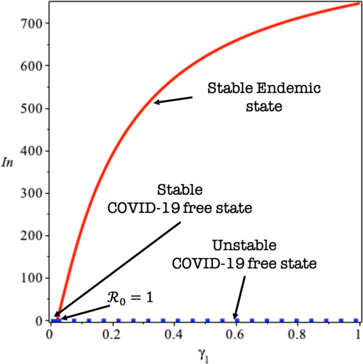
To illustrate the result of Theorems 3, 4, and 5, we give a bifurcation diagram of system 1 presented by detecting symptomatic variables with ${\mathcal{R}}_0$ in Fig. 2. To derive Fig. 2, we use parameter value as shown in Table 1 except ${\gamma }_1$ which used as the bifurcation parameter. When ${\gamma }_1<0.019$, then we have that ${\mathcal{R}}_0<1$, which gives a stable COVID-19 free equilibrium. When ${\gamma }_1=0.019$, zero eigenvalues appear, and change of stability appears when we can see that the COVID-19 free equilibrium becomes unstable, while the endemic equilibrium arises and locally stable.

Fig. 2.

Transcritical bifurcation diagram of system (1) using ${\gamma }_1$ as the bifurcation parameter.

Table 1.

The model parameters and initial model populations for COVID-19 epidemic outbreak with their biological definitions.

Symbols	Biological definitions	Estimated values	Sources
$S\left(0\right)$	Initial susceptible individuals	$11.081\times 10^6$	[26]
$A\left(0\right)$	Initial asymptomatic infected individuals	3.62	[26]
$I\left(0\right)$	Initial recorded symptomatic infected individuals	1	[26]
$U\left(0\right)$	Initial unrecorded symptomatic infected individuals	4.13	[26]
$R\left(0\right)$	Initial recovered individuals	0	[26]
${\beta }_1$	Transition rate between susceptible and asymptomatic infected individuals	$4.5\times 10^{-7}$	Fixed
${\beta }_2$	Transition rate between susceptible and unreported symptomatic infected individuals	$1.45\times 10^{-6}$	Fixed
${\beta }_3$	Transition rate between susceptible and reported symptomatic infected individuals	$8.68\times 10^{-8}$	[27]
$\delta$	Transition rate between asymptomatic infected and unreported symptomatic infected	0.0285	[26]
${\gamma }_1$	Transition rate between asymptomatic infected and reported symptomatic infected	0.1142	[26]
${\gamma }_2$	Transition rate between unreported symptomatic and reported symptomatic infected individuals	0.35	Fixed
${\eta }_1$	The recovery rate of unreported asymptomatic infected case	0.13978	[28]
${\eta }_2$	The recovery rate of unreported symptomatic infected case	0.2	Fixed
${\eta }_3$	The recovery rate of reported symptomatic infected case	0.33029	[28]
$\xi$	The reported and unreported symptomatic death rate	$1.7826\times 10^{-5}$	[28]

Discussion on ${\mathcal{R}}_0$

Based on Theorem 3, Theorem 4, the basic reproduction number in (3) determines the existence or disappearance of COVID-19. This ${\mathcal{R}}_0$ formed by three-component of a specific infection. The first component is ${\mathcal{R}}_{\text{asymptomatic}}=\frac{{\beta }_1\Lambda }{\mu (\delta +{\eta }_1+{\gamma }_1)}$, which described a number of new infection from direct contact between a susceptible individual with the asymptomatic individual during its infection period. To reduce this local basic reproduction number, various ways can be adopted, i.e., such as reducing $\beta$ to avoid infection with the asymptomatic individual. Unfortunately, the asymptomatic individual does not show any symptoms; therefore, avoid contact with this type of infected individual is difficult to be estimated. Therefore, the only way is to reduce random contact between each individual, whether it is a healthy or infected individual. In several countries [31], the government is campaigning for the use of medical masks to all people, regardless of whether they are infected or healthy individuals. The other way to reduce ${\mathcal{R}}_{\text{asymptomatic}}$ is to enlarging the rate of rapid-test ${\gamma }_1$. As mentioned before, the purpose of this rapid-test intervention is to map the infected individuals (asymptomatic and symptomatic), so several actions can be done to these individuals to prevent further infection. Enlarging ${\gamma }_1$ will help the government to be able to focus all health measures on this individual group, such as monitoring self-quarantine, isolation in hospitals, and so forth. The long-term effect is that the government can reduce the number of infections in the field from this group of individuals. Another way to reduce ${\mathcal{R}}_{\text{asymptomatic}}$ is by increasing the recovery rate ${\eta }_1$. Since these individuals do not show any symptoms, no medical intervention cannot be given to asymptomatic individuals. Therefore, encourage a healthy lifestyle to enhance self immunity through a media campaign is a reasonable option.

The second component in ${\mathcal{R}}_0$ is ${\mathcal{R}}_{\text{undetected}}$, which describes new infection from the unreported symptomatic cases during its infection period. Since $\frac{\partial {\mathcal{R}}_{\text{undetected}}}{\partial \delta }=\frac{\Lambda {\beta }_2\left({\eta }_1+{\gamma }_1\right)}{\mu {\left(\delta +{\eta }_1+{\gamma }_1\right)}^2\left(\xi +{\eta }_2+{\gamma }_2\right)}>0$, reducing the progression rate $\delta$ will reduce ${\mathcal{R}}_{\text{undetected}}$. In COVID-19, the incubation period estimated between 2–14 days [32]. Smaller $\delta$ means that the infection needs a longer time to show the symptoms. The other way except increasing rapid-test rate ${\gamma }_2$, to reduce ${\mathcal{R}}_{\text{undetected}}$ can be done by improving the quality and quantity of health services in hospitals, which our model represents, i.e., by reducing the death race induced by COVID-19 $\left(\xi \right)$ and increasing recovery rate $\left({\eta }_3\right)$. By increasing the capacity of the hospital, more infected individuals can get proper medical treatment, which is expected to reduce the rate of death due to disease, and shorten the duration of infection.

The third component in ${\mathcal{R}}_0$ is ${\mathcal{R}}_{\text{detected}}$ which describes a new infection caused by symptomatic reported cases during its infection period. Here, note that this class is monitored by the government, whether it in the hospital, or monitored by the government tracking system to conduct self-quarantine in their home. This intervention will reduce ${\beta }_3$. Discipline implementation of this contact reduction will reduce ${\beta }_3$ significantly, and more easy to be monitored compared with minimizing ${\beta }_1$ and ${\beta }_2$.

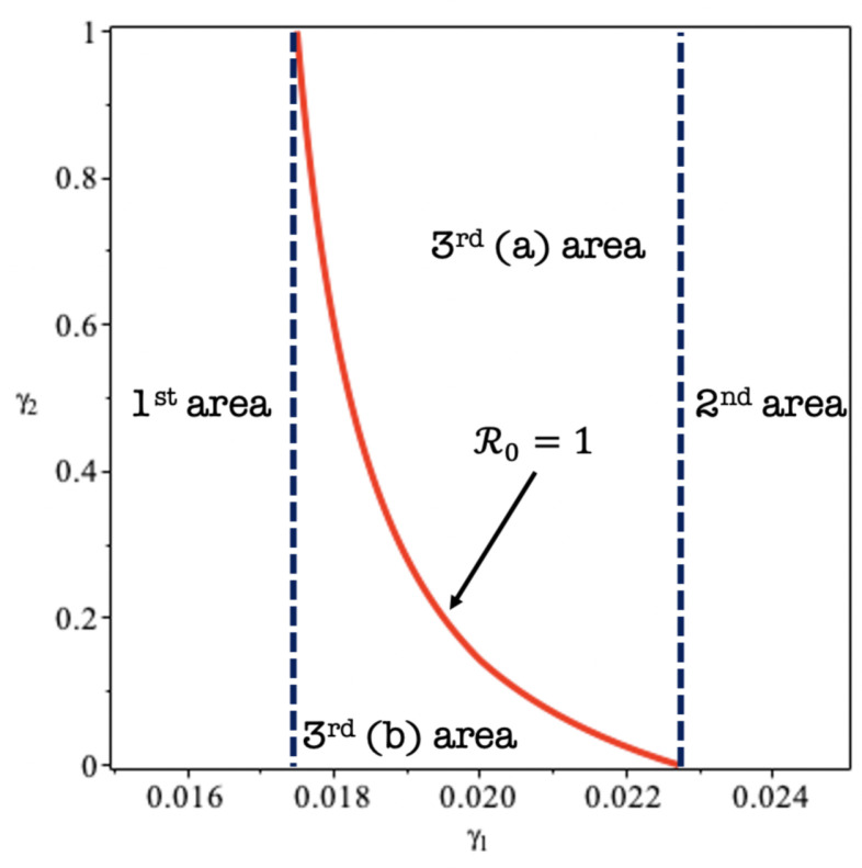
To finalize our discussion on ${\mathcal{R}}_0$, we perform a sensitivity analysis of ${\mathcal{R}}_0$ respect to ${\gamma }_1$ and ${\gamma }_2$. Using parameters value in Table 1 except ${\gamma }_1$ and ${\gamma }_2$, we plot a condition of ${\mathcal{R}}_0=1$ on ${\gamma }_1-{\gamma }_2$ plane in Fig. 3. Since $\frac{\partial {\mathcal{R}}_0}{\partial {\gamma }_1}$ and $\frac{\partial {\mathcal{R}}_0}{\partial {\gamma }_2}$ are negative, the 2nd and $3$rd(a) area represents a combination of ${\gamma }_1$ and ${\gamma }_2$ and gives ${\mathcal{R}}_0<1$, while 1st and $3$rd(b) area representing a condition when ${\mathcal{R}}_0>1$. The first information that we can take from Fig. 3 is that ${\gamma }_1$ is more sensitive in determining ${\mathcal{R}}_0$ rather than ${\gamma }_2$. It means that rapid-test intervention into asymptomatic individuals is more advisable to encourage for the implementation in the field. The reason is this, by bringing/identify the infected individuals in the field will give the government flexibility and more focus in the intervention. Another information that can be taken from Fig. 3 is that the existence of “useless” intervention, that is the 1st area. The 1st area (${\gamma }_1<0.0173$) representing a condition of ${\mathcal{R}}_0$ is always larger than one, no matter the value of ${\gamma }_2$. On the other hand, the 2nd area (${\gamma }_1>0.228$), represents an area when ${\mathcal{R}}_0$ is always less than one even though the government does not take a rapid-test ${\gamma }_2$ in unreported symptomatic individual. If the government only implements ${\gamma }_1$ in the area between 0.0173 and 0.228, then implementation of ${\gamma }_2$ must be taken carefully, since it can end up in an unsuccessful intervention ($3$rd(b) area) or the successful intervention ($3$rd(a) area). Therefore, implementing rapid-test need a very careful justification for the implementation, since a large rapid-test intervention leads to a very costly intervention, but small rapid-test could end up in an unsuccessful intervention.

Fig. 3.

A condition of ${\mathcal{R}}_0$ respect to ${\gamma }_1$ and ${\gamma }_2$.

Sensitivity analysis

Consider a system of differential equations

$$\begin{array}{c}\frac{d{x}_j}{dt}=h_j(x,\alpha ),\hfill \end{array}$$ (13)

where $x\in {\mathbb{R}}^m$ and $\alpha \in {\mathbb{R}}^n$. The functions $h_j,j=1,2,\dots ,m$ are often non-linear therefore model differential equations may not solve analytically. An important technique to analyze system (13) is the idea of sensitivity analysis. According to this approach, the sensitivity of each variable concerning parameters can be calculated. The main equation of sensitivity is given below

$$\begin{array}{c}{s}_{jp}=\frac{\partial x_j}{\partial {\alpha }_p}=\underset{\Delta {\alpha }_p\to 0}{lim}\frac{x_j({\alpha }_p+\Delta {\alpha }_p)-x_j\left({\alpha }_p\right)}{\Delta {\alpha }_p}.\hfill \end{array}$$ (14)

The first order derivatives given in Eq. (14) represent the time-dependent sensitivities of all variables $\{x_j,j=1,2,\dots ,m\}$ with respect to each parameter value $\{{\alpha }_p,p=1,2,\dots ,n\}$. Furthermore, the differential equations can be solved for sensitivity coefficients as below

$$\begin{array}{c}\frac{\partial s_{jp}}{\partial t}=\frac{\partial }{\partial t}\left(\frac{\partial x_j}{\partial {\alpha }_p}\right)=\frac{\partial }{\partial {\alpha }_p}\left(\frac{\partial x_j}{\partial t}\right)=\frac{\partial }{\partial {\alpha }_p}\left(h_j\left(x\left(t\right)\right),\alpha \right).\hfill \end{array}$$ (15)

Using the chain rule of differentiation, Eq. (15) can be further driven and the sensitivity equations take the Jacobian matrix as follows

$$\begin{array}{c}\dot{\mathcal{S}}={\mathcal{H}}_{{\alpha }_p}+\mathcal{J}.\mathcal{S},p=1,2,\dots ,n,\hfill \end{array}$$ (16)

where the matrices $\mathcal{S},{\mathcal{H}}_{{\alpha }_p}$ and $\mathcal{J}$ are defined by

$$\mathcal{S}=\left(\begin{array}{c}\hfill \frac{\partial x_1}{\partial {\alpha }_p}\hfill \\ \hfill \frac{\partial x_2}{\partial {\alpha }_p}\hfill \\ \hfill ⋮\hfill \\ \hfill \frac{\partial x_m}{\partial {\alpha }_p}\hfill \end{array}\right),{\mathcal{H}}_{{\alpha }_p}=\left(\begin{array}{c}\hfill \frac{\partial h_1}{\partial {\alpha }_p}\hfill \\ \hfill \frac{\partial h_2}{\partial {\alpha }_p}\hfill \\ \hfill ⋮\hfill \\ \hfill \frac{\partial h_m}{\partial {\alpha }_p}\hfill \end{array}\right),\mathcal{J}=\left(\begin{array}{cccc}\hfill \frac{\partial h_1}{\partial x_1}\hfill & \hfill \frac{\partial h_1}{\partial x_2}\hfill & \hfill \cdots \hfill & \hfill \frac{\partial h_1}{\partial x_m}\hfill \\ \hfill \frac{\partial h_2}{\partial x_1}\hfill & \hfill \frac{\partial h_2}{\partial x_2}\hfill & \hfill \cdots \hfill & \hfill \frac{\partial h_2}{\partial x_m}\hfill \\ \hfill ⋮\hfill & \hfill ⋮\hfill & \hfill \ddots \hfill & \hfill ⋮\hfill \\ \hfill \frac{\partial h_m}{\partial x_1}\hfill & \hfill \frac{\partial h_m}{\partial x_2}\hfill & \hfill \cdots \hfill & \hfill \frac{\partial h_m}{\partial x_m}\hfill \end{array}\right).$$

For more details and applications of sensitivity analysis in the field of systems biology, the readers are refereed to [33], [34], [35], [36], [37], [38], [39], [40]. The local sensitivity values are given in Eq. (16) can be computed using SimBiology Toolbox in MATLAB with three different techniques: non-normalizations, half normalizations, and full normalizations. Accordingly, in a complicated modeling case like new coronavirus dynamics, it is necessary to pay attention to sensitivity analysis more accurately and widely. This helps us to identify the key critical model parameters and to improve model dynamics.

Computational results

Mathematical models and computational simulations help and provide a good environment to analyze high dimensional models of infectious diseases. Such models may help biologists to predict future model dynamics and identify critical model parameters. The suggested mathematical models of COVID-19 are effective tools that give estimations and suggestions about controlling the virus and further preventions more effectively and widely. The values of parameters and initial populations in this study are obtained from the WHO situation reports (the National Health Commission of the Republic of China) presented in [26], [27], [28].

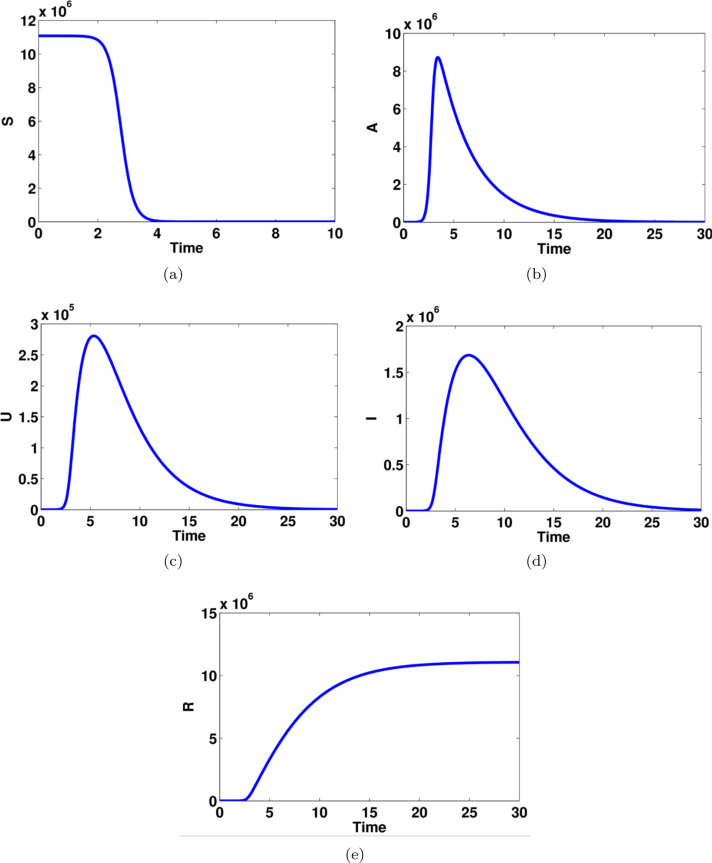
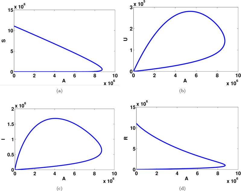
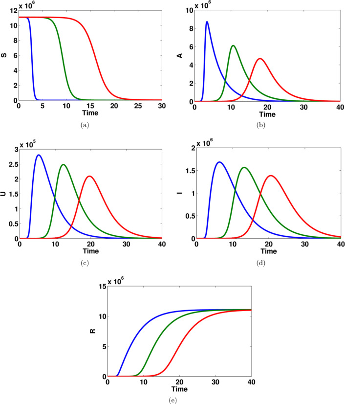
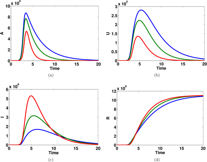
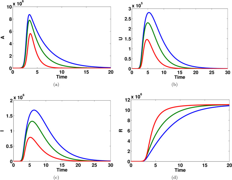
There are some numerical approximate solutions of the model equations (1) for different parameters and initial populations using System Biology Toolbox(SBedit) for MATLAB; see Fig. 4, Fig. 5, Fig. 6, Fig. 7, Fig. 8, Fig. 9, Fig. 10, Fig. 11. Accordingly, different model dynamics for initial populations are obtained based on changing the value of model parameters. Results in this study provide a good step forward in predicting the model dynamics in the future for development programs, interventions and health care strategies.

Fig. 4.

Computational simulations for the model states given in system (1) of the COVID-19 using MATLAB; there are model dynamics of (a) susceptible individuals, (b) asymptomatic infected individuals, (c) unreported symptomatic infected individuals, (d) reported symptomatic infected individuals, (e) recovered individuals.

Fig. 5.

Computational simulations for the model states given in system (1) of the COVID-19 using MATLAB; there is the relationship between the asymptomatic infected people and (a) susceptible individuals, (b) unreported symptomatic infected individuals, (c) reported symptomatic infected individuals, (d) recovered individuals.

Fig. 6.

The effect of transition rate ${\beta }_1$ on (a) susceptible individuals (b) asymptomatic infected individuals, (c) unreported symptomatic infected individuals, (d) reported symptomatic infected individuals (e) recovered individuals, in computational simulations using MATLAB parameters used ${\beta }_1=4.5\times 10^{-7}$ for blue lines, ${\beta }_1=1.2\times 10^{-7}$ for green lines and ${\beta }_1=5.2\times 10^{-8}$ for red lines. (For interpretation of the references to color in this figure legend, the reader is referred to the web version of this article.)

Fig. 7.

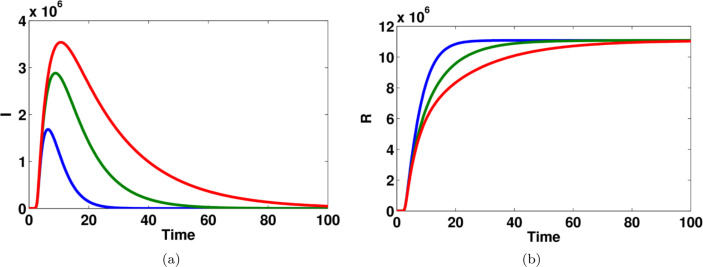
The effect of transition rate ${\gamma }_1$ on (a) asymptomatic infected individuals, (b) unreported symptomatic infected individuals, (c) reported symptomatic infected individuals (d) recovered individuals, in computational simulations using MATLAB parameters used ${\gamma }_1=0.1142$ for blue lines, ${\gamma }_1=0.3$ for green lines and ${\gamma }_1=0.9$ for red lines. (For interpretation of the references to color in this figure legend, the reader is referred to the web version of this article.)

Fig. 8.

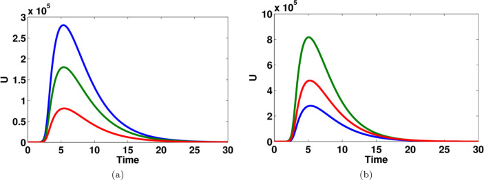
The effect of transition rate ${\eta }_1$ on (a) asymptomatic infected individuals, (b) unreported symptomatic infected individuals, (c) reported symptomatic infected individuals (d) recovered individuals, in computational simulations using MATLAB parameters used ${\eta }_1=0.13978$ for blue lines, ${\eta }_1=0.3$ for green lines and ${\eta }_1=0.8$ for red lines. (For interpretation of the references to color in this figure legend, the reader is referred to the web version of this article.)

Fig. 9.

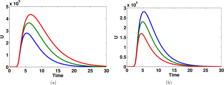
The effect of transition rate $\delta$ on (a) unreported symptomatic infected individuals, parameter used $\delta =0.0285$ (blue line), $\delta =0.018$ (green line), $\delta =0.008$ (red line), (b) unreported symptomatic infected individuals, parameter used $\delta =0.09$ (red line), $\delta =0.05$ (green line), $\delta =0.0285$ (blue line). (For interpretation of the references to color in this figure legend, the reader is referred to the web version of this article.)

Fig. 10.

The effect of transition rate ${\eta }_3$ on (a) reported symptomatic infected individuals (b) recovered individuals, in computational simulations using MATLAB parameters used ${\eta }_3=0.33029$ for blue lines, ${\eta }_3=0.1$ for green lines and ${\eta }_3=0.05$ for red lines. (For interpretation of the references to color in this figure legend, the reader is referred to the web version of this article.)

Fig. 11.

The effect of transition rate ${\gamma }_2$ and ${\eta }_2$ on unreported symptomatic infected individuals in computational simulations using MATLAB parameters used (a) ${\gamma }_2=0.35$ for blue lines, ${\gamma }_2=0.15$ for green lines and ${\gamma }_2=0.05$ for red lines, (b) ${\eta }_2=0.2$ for blue lines, ${\eta }_2=0.4$ for green lines and ${\eta }_2=0.8$ for red lines. (For interpretation of the references to color in this figure legend, the reader is referred to the web version of this article.)

To perform our numerical experiments in this section, due to a short time interval of simulation, we ignore new-born and natural death rate in our model. Therefore, we have that $A=0$ and $\mu =0$. With this assumption, our model now read as:

$$\begin{array}{c}\frac{dS}{dt}=-S\left({\beta }_{1}A+{\beta }_{2}U+{\beta }_{3}I\right),\hfill \\ \frac{dA}{dt}=S\left({\beta }_{1}A+{\beta }_{2}U+{\beta }_{3}I\right)-\delta A-{\gamma }_{1}A-{\eta }_{1}A,\hfill \\ \frac{dU}{dt}=\delta A-{\gamma }_{2}U-{\eta }_{2}U-\xi U,\hfill \\ \frac{dI}{dt}={\gamma }_{1}A+{\gamma }_{2}U-{\eta }_{3}I-\xi I,\hfill \\ \frac{dR}{dt}={\eta }_{1}A+{\eta }_{2}U+{\eta }_{3}I.\hfill \end{array}$$ (17)

The model dynamics of susceptible, asymptomatic infected, reported symptomatic infected, unreported symptomatic infected and recovered individuals are shown in Fig. 4. The number of susceptible individuals decreases dramatically and becomes stable after four days while the dynamics of recovered people increase gradually and get flat after 15 days. Interestingly, the number of asymptomatic infected individuals reaches a high level after 5 days while the number of infected people in both reported and unreported symptomatic are dramatically changed between 3 days to 15 days. Furthermore, Fig. 5 explains the relationship between asymptomatic infected people with the other groups in the COVID-19. There are almost the same model dynamics for reported and unreported symptomatic states whereas there are slightly different model dynamics for susceptible and recovered groups.

Fig. 6 shows that the impact of the transition rate ${\beta }_1$ on all model variables. The effect of this parameter can easily occur on in the dynamics of the model states. For example, if the value of ${\beta }_1$ is increased then the number of asymptomatic, unreported symptomatic and reported symptomatic infected people are also increased, see Fig. 6(b,c,d). Also, the dynamics of susceptible and recovered people become stable when the value of this parameter becomes larger and larger, see Fig. 6(a) and (e).

Fig. 7 shows that the impact of transition rate ${\gamma }_1$ on asymptomatic infected people, reported symptomatic infected, unreported symptomatic infected, and recovered people. The effect of this parameter can easily occur on the variables $A,I,U$ and $R$. It can be seen that the model dynamics for such states become flattered when the value of ${\gamma }_1$ is increased, see Fig. 7(a,b,d). On the other hand, the number of reported symptomatic people becomes larger when the value of this parameter is increased, see Fig. 7(c). This is an important key element for controlling this disease.

The impact of transition rate ${\eta }_1$ on asymptomatic infected, reported symptomatic infected, unreported symptomatic infected, and recovered people is shown in Fig. 8. Intestinally, the number of infected people in $A,U,I$ groups is dramatically increased when the value of ${\eta }_1$ gets smaller, this is illustrated in Fig. 8(a,b,c). Furthermore, the dynamic of recovered individuals reaches stable very quickly when this parameter becomes large, see Fig. 8(d).

Fig. 9 shows that the impact of parameter $\delta$ on the dynamics of unreported symptomatic infected people. The number of infected people is significantly changed for different values of $\delta$. The effect of transition rate ${\eta }_3$ on reported symptomatic infected individuals and recovered individuals are computed and given in Fig. 10. Moreover, the effect of transition rate ${\gamma }_2$ and ${\eta }_2$ on unreported symptomatic infected individuals are shown in Fig. 11.

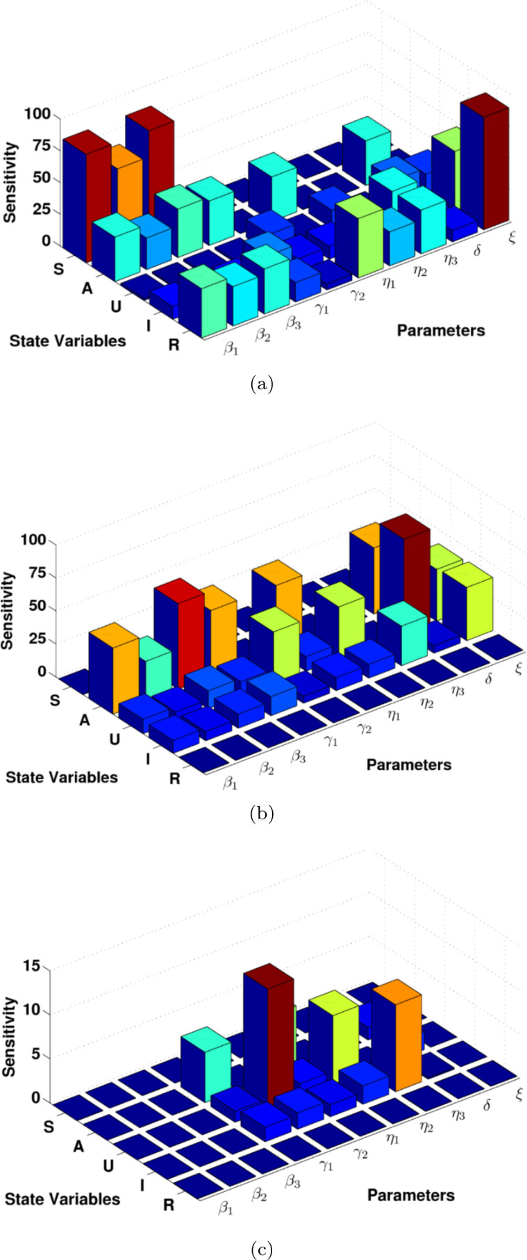
The idea of sensitivity analysis has an important role in identifying the model critical element. The main equation of local sensitivity is presented in Eq. (16). We use SimBiology Toolbox for MATLAB to calculate the local sensitivity of each model state concerning model parameters for the model equations (1). We compute the model sensitivities using three different techniques: non-normalizations, half normalizations and full normalizations; see Fig. 12. Interestingly, results provide us further understanding of the model and helps us to identify the key critical model parameters. For example, it generally seems that the susceptible, asymptomatic infected, recovered individuals are more sensitive to the set of model parameters compared to the reported and unreported symptomatic individuals, this result is based on non-normalization approach, see Fig. 12(a). Another interesting result is that the group of asymptomatic, reported symptomatic, unreported symptomatic people are very sensitive to almost all model parameters, see Fig. 12(b). This is an effective step to identify the model critical parameters for controlling the spread of COVID-19. Accordingly, the parameters $\{{\gamma }_1,{\gamma }_2,{\eta }_1,{\eta }_2,{\eta }_3\}$ are the key critical elements for understanding and to prevent this disease because they are very sensitive according to full normalization method presented in Fig. 12(c). As a result, identifying critical model parameters in this study based on computational simulations is an effective way to further study the model practically and theoretically and give some suggestions for future improvements of the novel coronavirus vaccination programs, interventions and controlling the spread of disease.

Fig. 12.

The sensitivity of each model state with respect to model parameters in computational simulations for the coronavirus disease (COVID-19); (a) non-normalization sensitivity, (b) half normalization sensitivity, (c) full normalization sensitivity.

Optimal control problem

Characterization of the optimal control problem

In this section, we analyze the optimal control problem related to the model (1). This optimal control approach aims to minimize the number of an infected individual $(A,U,R)$ using rapid-test intervention. As explained in Section “A Mathematical Model of COVID-19” that with the rapid-test, policymakers could map and detect the infected individual; hence, the controlled isolation could be implemented to these individuals to avoid contact with a susceptible individual. Therefore, we re-define ${\gamma }_1$ and ${\gamma }_2$ in system (1) as a time-dependent parameter $u_1\left(t\right),u_2\left(t\right)$, respectively. Due to a short time of interval simulation and short term of COVID-19 pandemic, we neglect natural new-born and the natural death rate from our model, similarly with Section “Computational Results”. Also, since $R$ does not appear in another part of the equation in (17) except in $dR/dt$, we may ignore $R$ from our optimal control problem. Therefore, system (17) now read as:

$$\begin{array}{c}\frac{dS}{dt}=-S\left({\beta }_{1}A+{\beta }_{2}U+{\beta }_{3}I\right),\hfill \\ \frac{dA}{dt}=S\left({\beta }_{1}A+{\beta }_{2}U+{\beta }_{3}I\right)-\delta A-u_1\left(t\right)A-{\eta }_{1}A,\hfill \\ \frac{dU}{dt}=\delta A-u_2\left(t\right)U-{\eta }_{2}U-\xi U,\hfill \\ \frac{dI}{dt}=u_1\left(t\right)A+u_2\left(t\right)U-{\eta }_{3}I-\xi I,\hfill \\ \hfill \end{array}$$ (18)

Mathematically, our goal is to find an optimal rate of rapid test which minimize the following cost functional:

$$\mathcal{J}(u_1,u_2)={\int }_0^{t_f}\left[a_{1}A+a_{2}U+a_{3}I+\frac{1}{2}{b}_1{u}_1^2+\frac{1}{2}{b}_2{u}_2^2\right]dt.$$ (19)

The first three-component in the integrand is a cost related to a high number of COVID-19 infections in the community, while the last to component related to rapid-test intervention. Note that $a_1,a_2,a_3,b_1$, and $b_2$ are the weight constant that will balance each component in this cost function.

Here we seek an optimal solution $\left(u_1^{\ast },u_2^{\ast }\right)$ such that

$$\mathcal{J}(u_1^{\ast },u_2^{\ast })=min\left\{\mathcal{J}(u_1,u_2)\in \mathcal{U}|\right\},$$ (20)

where $\mathcal{U}=\left\{u_i|u_i\text{ is Lebesgue measurable and}0\le u_i^{min}\le u_i\right)$ $\left(\le u_2^{max}\le 1\right\}$ be the set of admissible control. To investigate the existence of optimal control, we use Pontryagin’s Maximum Principle to govern the necessary condition of the optimal control problem. The Lagrangian for the optimal system (18) can be defined as:

$$\mathcal{L}(S,A,I,U,{\lambda }_j,u_i)=a_{1}A+a_{2}U+a_{3}I+\frac{1}{2}{b}_1{u}_1^2+\frac{1}{2}{b}_2{u}_2^2={\lambda }_1\left[-S\left({\beta }_{1}A+{\beta }_{2}U+{\beta }_{3}I\right)\right]+{\lambda }_2\left[S\left({\beta }_{1}A+{\beta }_{2}U+{\beta }_{3}I\right)-\delta A-u_1\left(t\right)A-{\eta }_{1}A\right]+{\lambda }_3\left[\delta A-u_2\left(t\right)U-{\eta }_{2}U-\xi U\right]+{\lambda }_4\left[u_1\left(t\right)A+u_2\left(t\right)U-{\eta }_{3}I-\xi I\right],$$

where ${\lambda }_j$ for $j=1,2,3,4$ are the costate variable related to $S,A,U,I$, respectively. The costate variable ${\lambda }_j$ satisfies the following system of ordinary differential equations:

$$\frac{d{\lambda }_1}{dt}=-\frac{\partial \mathcal{L}}{\partial S}=\left({\beta }_{1}A+{\beta }_{2}U+{\beta }_{3}I\right)\left({\lambda }_2-{\lambda }_1\right),$$

$$\frac{d{\lambda }_2}{dt}=-\frac{\partial \mathcal{L}}{\partial A}=-a_1+{\beta }_{1}S\left({\lambda }_1-{\lambda }_2\right)+\delta \left({\lambda }_2-{\lambda }_3\right)+u_1\left({\lambda }_2-{\lambda }_4\right)+{\eta }_1{\lambda }_2,$$ (21)

$$\frac{d{\lambda }_3}{dt}=-\frac{\partial \mathcal{L}}{\partial U}=-a_2+{\beta }_{2}S({\lambda }_1-{\lambda }_2)+u_2({\lambda }_3-{\lambda }_4)+(\xi +{\eta }_2){\lambda }_3,$$

$$\frac{d{\lambda }_4}{dt}=-\frac{\partial \mathcal{L}}{\partial I}=-a_3+{\beta }_{3}S({\lambda }_1-{\lambda }_2)+(\xi +{\eta }_3){\lambda }_4,$$

with the transversality condition ${\lambda }_j\left(t_f\right)=0$ for $j=1,2,3,4$. Using the optimality condition $\frac{\partial \mathcal{L}}{\partial u_i}=0$, we get:

$$u_1^{†}=\frac{A({\lambda }_2-{\lambda }_4)}{b_1},$$

$$u_2^{†}=\frac{U({\lambda }_3-{\lambda }_4)}{b_2}.$$

Taking into account the lower and upper bound for $u_1$ and $u_2$, we get the characterization:

$$u_1^{\ast }=min\left\{max\left\{\frac{A({\lambda }_2-{\lambda }_4)}{b_1},\underset{1}{\overset{min}{u}}\right\},\underset{1}{\overset{max}{u}}\right\},$$

$$u_2^{\ast }=min\left\{max\left\{\frac{U({\lambda }_3-{\lambda }_4)}{b_2},\underset{2}{\overset{min}{u}}\right\},\underset{2}{\overset{max}{u}}\right\}.$$ (22)

Numerical experiment on the optimal control problem

The optimal control system which involves the system of state variables in (18), costate variables in (21), and optimal characterization in (22) is analyzed using the Runge–Kutta forward–backward iterative numerical approximation method [21], [23], [41]. The idea of this method as follows. First, give an initial guess for control variables $u_1$ and $u_2$ for all time $t\in [0,t_f]$. Using this value, and the initial condition for state variables, solve system (18) forward in time to find values of state variables in all-time $t\in [0,t_f]$, and calculate the cost function (19). Next, solve the costate system (21) backward in time using the transversality condition of costate variables, an initial guess of $u_i$ and solution of state variables from the previous step. Next, update the control variables using Eq. (22). Repeat this scheme until the convergence criteria achieved. In this article, the terminate condition is until the error of the optimal solution ${\varphi }^{\ast }=\left\{S^{\ast },A^{\ast },U^{\ast },I^{\ast },u_1^{\ast },u_2^{\ast }\right\}$ in iteration-$k$ is less than small constant $\delta$, or in this case:

$$\text{error}=\frac{‖{\varphi }^{\left(k\right)}-{\varphi }^{(k-1)}‖}{‖x^{\left(k\right)}‖}<\delta .$$

For the base-case, we choose the weight cost:

$$(a_1,a_2,a_3,b_1,b_2)=(10,10,1,10^6,10^5).$$

Note that $a_1$ and $a_2$ are larger than $a_3$ because it is quite difficult for the policymaker to handle the undetected crises. Furthermore, we have that $c_1>c_2$ since the rapid test for the asymptomatic individual is easier to implement if the candidate had already shown the symptoms. We run our simulation for $t\in [0,120]$.

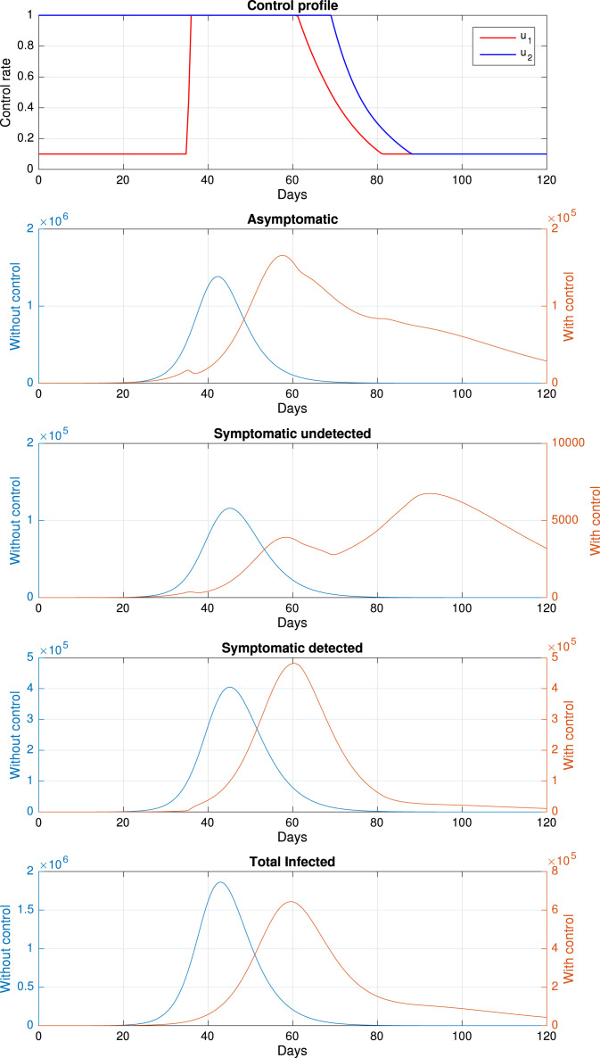
For the base case, we use parameter value as shown in Table 1, and the numerical results are given in Fig. 13, and the final number of infected individuals at $t=30$, total cost function (19), and a number of an averted infected individual given in Table 2. Please note that we use two different y-axes to identify the number of the infected individual, with and without control, since the scale of an infected individual without control is almost ten times larger than with controls. It can be seen that the time-dependent control succeeds in suppressing the number of infected individuals in all classes. The Control profile for $u_1$ and $u_2$ is relatively different. It can be seen that rapid test for the symptomatic individual $\left(u_2\right)$ should be given at a maximum rate since the early time of simulation, and start to decrease to it minimum value after day 70, where the total of infected individuals are already decreasing. On the other hand, rapid-test for asymptomatic individual start to be implemented at day 35 when a total of individual infected start to increase, and it starts to decrease when the number of asymptomatic individuals also shows a decreasing trend. It is interesting to see that the dynamic of the symptomatic individual has three outbreaks. The first outbreak occurs as a consequence of $u_1$ start to increase in day 35, while the second outbreak occurs when $u_1$ starts to decrease to its minimum value in day 62. When $u_2$ starts to decrease in day 70, the infected population will start to increase, and the symptomatic class will reach the third outbreak on day 90. Using the control profile, which depends on time, as shown in Fig. 13, we can avoid new cases as much as 138 thousand cases with the cost of intervention more than 50% cheaper than without the intervention.

Fig. 13.

Numerical simulation of the optimal control problem of the system (18) for the base-case.

Table 2.

Numerical result for the base-case in Fig. 13.

Case	$\mathcal{J}$	New infection averted
No control	$2.43\times 10^6$	–
Time-dependent control	$4.87\times 10^5$	$138000$

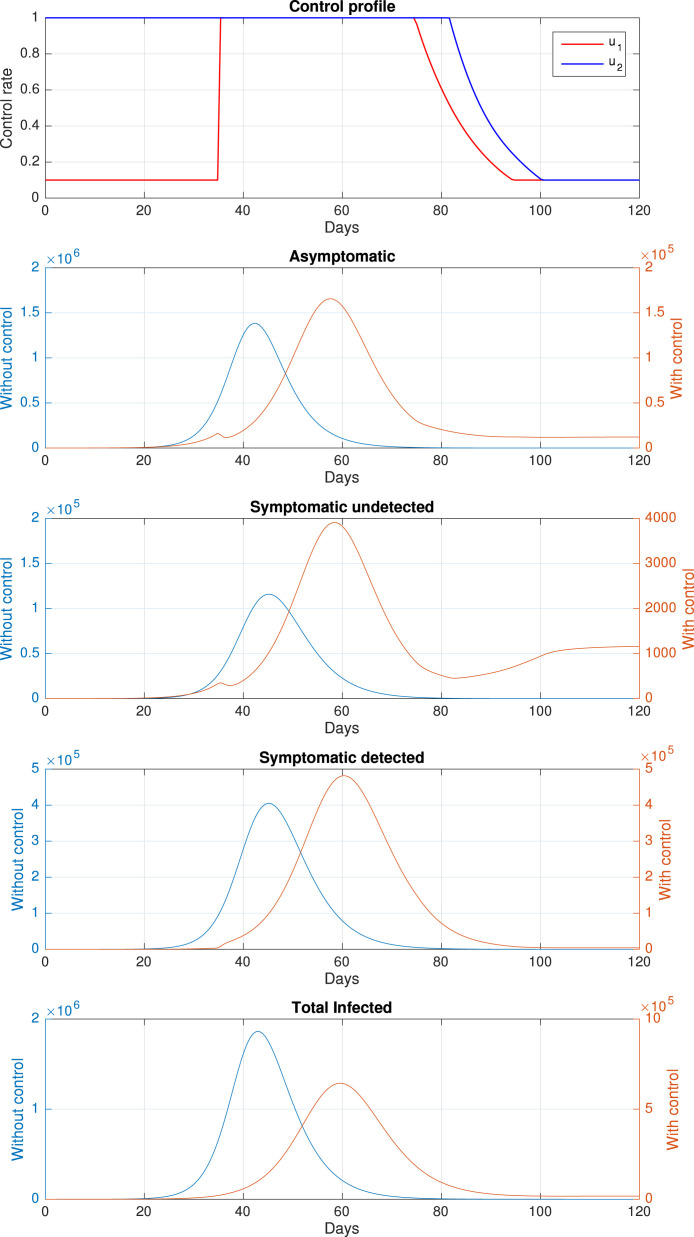
Our second simulation conducted to see the impact of a cheaper rapid-test cost on the dynamic of the infected population. To do this, we redefine the weight parameter of the base case as $(a_1,a_2,a_3,b_1,b_2)=(10,10,1,10^5,10^4)$, while the other parameters remain the same. It can be seen that $b_1$ and $b_2$ for this scenario are ten times smaller than in the base-case. The dynamic of the infected population and the control profile can be seen in Fig. 14, and the numerical results are shown in Table 3. Similar to the base-case scenario, the time-dependent control could avoid more than one hundred thousand new cases. As a consequence of a cheaper rapid-test cost, it can be seen that $u_1$ and $u_2$ can remain at the maximum rate for a longer period than in the base-case. Furthermore, we can see that instead of having three outbreak as in the base-case, the symptomatic undetected case only have two outbreak in this scenario. Therefore, we can conclude that a massive implementation of rapid-test as a consequence of a cheaper cost for the implementation could prevent a future outbreak of COVID-19.

Fig. 14.

Numerical simulation of the optimal control problem of system (18) when $b_1$ and $b_2$ is smaller ten times than in the base-case.

Table 3.

Numerical result for Fig. 14.

Case	$\mathcal{J}$	New infection averted
No control	$2.45\times 10^6$	–
Time-dependent control	$5.5\times 10^5$	$157740$

Application of the proposed model to forecast some COVID-19 incidence data

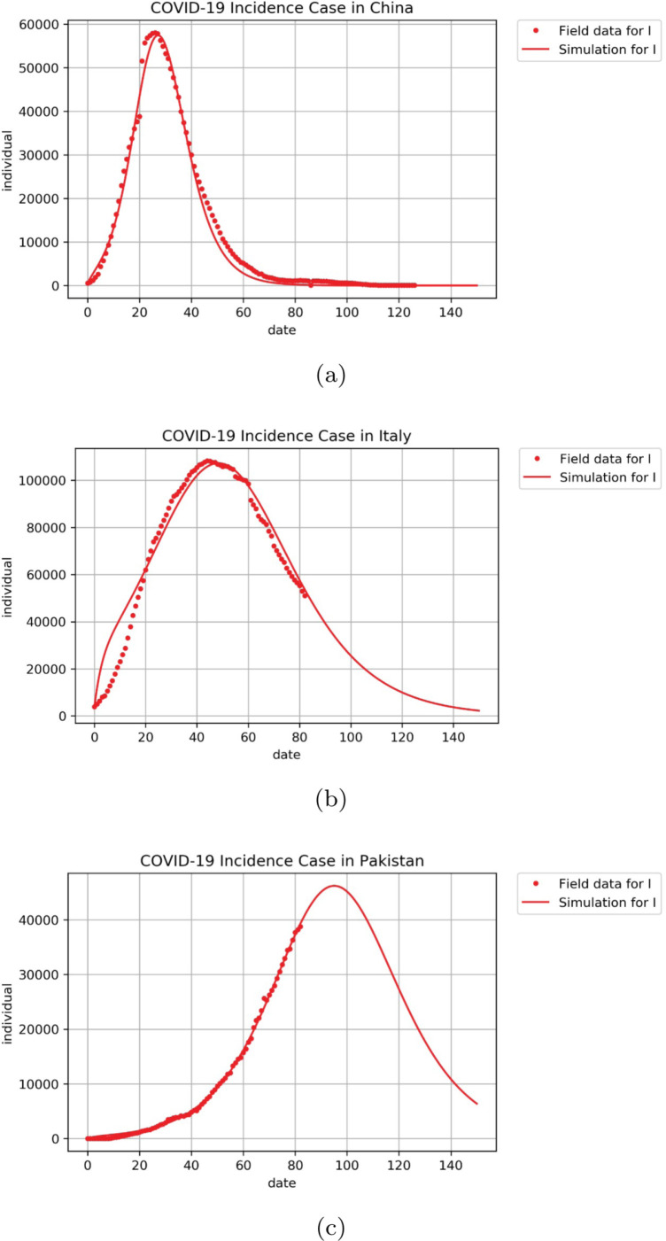
In this section, we present some examples of how our model in (17) can fit COVID-19 incidence data. The incidence data used in this article can be accessed in [42]. We fit the daily infected data to compartment $I$ in the proposed model (17) for the early outbreak period. We use parameter value as shown in Table 1, except ${\beta }_1,{\beta }_2$, and ${\beta }_3$ which we estimated from the real data. We use COVID-19 incidence data from China (Date of 22 January 2020–27 May 2020), Italy (Date of 6 March 2020–27 May 2020) and Pakistan (6 March 2020–27 May 2020). To fit these real incidence data, we use the software MATLAB. The results are shown in Fig. 15, and the parameters that been estimated can be seen in Table 4. It can be seen that our model could fit the Incidence data in China. For data of Italy, our model suggests that the disease In Italy shows a decreasing trend and will tend to zero cases approximately after day 150 of simulation (Late of July 2020). On the other hand, our numerical results for Pakistan data show that our proposed model can capture the dynamics of COVID-19 in the early period of the outbreak.

Fig. 15.

Confirmed COVID-19 data (dotted) vs. simulation of model (17) in (a) China, (b) Italy and (c) Pakistan.

Table 4.

Numerical result for Fig. 15.

Country	${\beta }_1$	${\beta }_2$	${\beta }_3$
China	$4.015\times 10^{-8}$	$7.4827\times 10^{-8}$	$8.04\times 10^{-9}$
Italy	$3.768\times 10^{-8}$	$5.4767\times 10^{-8}$	$7.536\times 10^{-9}$
Italy	$1.817\times 10^{-7}$	$3.634\times 10^{-7}$	$3.5\times 10^{-8}$

Conclusions

Let us summarized the discussion started with the mathematical modeling and concluded with the prime results, while all the data for studies are obtained from the WHO situation reports NHCRC.

• •Here we have modeled the dynamics of all possible cases of human to human transmission, i.e., susceptible, asymptomatic infected, reported symptomatic infected, unreported symptomatic infected, and recovered individuals to analyze accurate transmission dynamics of the COVID-19 outbreak.
• •The solutions of the model equations for different parameters and initial populations have been numerically approximated using System Biology Toolbox (SBedit) for MATLAB.
• •The modeling and simulation based on the suggested sensitivity analysis indicate that almost all model parameters may have a role in spreading this virus among susceptible, infected, recorded symptomatic, unrecorded symptomatic, and recovered individuals.
• •The effect of the control strategies on the model is analyzed graphically and analytically. From the analysis of the basic reproduction number, we found that rapid-test intervention, which aims to detect infected individuals among the human population, is promising to suppress the spread of the COVID-19. The success level of rapid-test also depending on how the government follows up the cases that have been detected with the help of rapid-test, for instance, with self-quarantine monitored for the infected individual if the case is not yet serious. Increasing the quality of the hospital by upgrading the capacity of the hospital or increase the number of medical staff can also increase the chance of COVID-19 eradication program.
• •The prospect of rapid test intervention to help the eradication program of COVID-19 analyzed using the optimal control theory. We find that a time-dependent rapid test intervention could reduce the number of new COVID-19 infection at a lower cost. We also find that rapid tests could reduce the size of future outbreak, delay the time of it appearance, furthermore, it also could eliminate the possibility of outbreak occurrence if the implementation of rapid-test is set to be adapted to the increasing number of infections.
• •The coronavirus, which is the cause of COVID-19, is very easy to mutate. Based on , until 2022, the virus variants for COVID-19 are divided into three, namely variants of concern (4 serotypes), Variants of Interest (3 serotypes), Variants under monitoring (7 serotypes), and De-escalated variants (27 serotypes). These serotype differences are shown in the virus’s physiology and its consequences on people infected with COVID-19, such as the speed it spreads, the response to the environment, and how dangerous the serotype is to humans. Therefore, further analysis is needed regarding these serotype differences. Differences in vaccine efficacy against different serotypes make it difficult to predict the dynamics of COVID-19 with simple models. Multiple variants model can be considered to understand this issue better.
• •Many types of vaccines have been introduced in various parts of the world. Not all communities in various countries accept this vaccination policy. In addition, several countries have not yet achieved the high vaccination coverage recommended by WHO. Based on this, the mathematical model in this paper needs to be developed by considering the complexity of this vaccination problem, such as differences in vaccine efficacy, multiple phases and vaccine booster, and others.

Results in this study provide a good step forward in predicting the model dynamics in the future for development programs, interventions, and health care strategies. For further development of the model, the reader could consider the existence of the maximum capacity of the hospital since the low capacity of the hospital will prolong the infection period. An application of optimal control problems to model the rate of rapid-test intervention as the time-dependent variable could be considered to handle the budget limitation on the COVID-19 eradication program.

Declaration of Competing Interest

The authors declare that they have no known competing financial interests or personal relationships that could have appeared to influence the work reported in this paper.

References

- 1.Geller C., Varbanov M., Duval RE. Human coronaviruses: insights into environmental resistance and its influence on the development of new antiseptic strategies. Viruses. 2012;4(11) doi: 10.3390/v4113044. PMC 3509683. PMID 23202515. [DOI] [PMC free article] [PubMed] [Google Scholar]
- 2.Zhu Na, Zhang Dingyu, Wang Wenling, Li Xingwang, Yang Bo, Song Jingdong, Zhao Xiang, Huang Baoying, Shi Weifeng, Lu Roujian, Niu Peihua. A novel coronavirus from patients with pneumonia in China, 2019. N Engl J Med. 2020;382(8):727–733. doi: 10.1056/NEJMoa2001017. PMC 7092803. PMID 31978945. [DOI] [PMC free article] [PubMed] [Google Scholar]
- 3.Li Q., Guan X., Wu P., Wang X., Zhou L., Tong Y., et al. Early transmission dynamics in Wuhan, China, of novel coronavirus-infected pneumonia. N Engl J Med. 2020 doi: 10.1056/NEJMoa2001316. [DOI] [PMC free article] [PubMed] [Google Scholar]
- 4.Wu JT., Leung K., Leung GM. Nowcasting and forecasting the potential domestic and international spread of the 2019-nCoV outbreak originating in Wuhan, China: a modelling study. Lancet. 2020 doi: 10.1016/S0140-6736(20)30260-9. [DOI] [PMC free article] [PubMed] [Google Scholar]
- 5.Tanne J.H., Hayasaki E., Zastrow M., Pulla P., Smith P., Rada A.G. Covid-19: how doctors and healthcare systems are tackling coronavirus worldwide. BMJ. 2020:368. doi: 10.1136/bmj.m1090. [DOI] [PubMed] [Google Scholar]
- 6.Lin Q., Zhao S., Gao D., Lou Y., Yang S., Musa S.S., Wang M.H., Cai Y., Wang W., Yang L., He D. A conceptual model for the coronavirus disease 2019 (COVID-19) outbreak in Wuhan, China with individual reaction and governmental action. Int J Infect Diseases. 2020;93:211–216. doi: 10.1016/j.ijid.2020.02.058. [DOI] [PMC free article] [PubMed] [Google Scholar]
- 7.Takian A., Raoofi A., Kazempour-Ardebili S. COVID-19 battle during the toughest sanctions against Iran. Lancet. 2020;395(10229):1035. doi: 10.1016/S0140-6736(20)30668-1. [DOI] [PMC free article] [PubMed] [Google Scholar]
- 8.Khoshnaw S.H.A. University Leicester-UK; 2015. Model reductions in biochemical reaction networks. (Ph.D. thesis) [Google Scholar]
- 9.Shahzad M., Sultan F., Ali S.I., Ali M., Azeem W. Physical assessments on chemically reacting species and reduction schemes for the approximation of invariant manifolds. J Molecular Liquids. 2019;285:237–243. doi: 10.1016/j.molliq.2019.03.031. [DOI] [Google Scholar]
- 10.Shahzad M., Sultan F. Advanced chemical kinetics. InTech; 2018. Complex reaction and dynamics. [DOI] [Google Scholar]
- 11.Shahzad M., Sultan F., Ali M., et al. Modeling multi-route reaction mechanism for surfaces: a mathematical and computational approach. Appl Nanosci. 2020 doi: 10.1007/s13204-020-01275-4. [DOI] [Google Scholar]
- 12.Shahzad M., Sultan F., Ali M., Khan W.A., Irfan M. Slow invariant manifold assessments in the multi-route reaction mechanism. J Molecular Liquids. 2019;284:265–270. doi: 10.1016/j.molliq.2019.03.179. [DOI] [Google Scholar]
- 13.Liu Y., Gayle A.A., Wilder-Smith A., Rocklöv J. The reproductive number of COVID-19 is higher compared to SARS coronavirus. J Travel Med. 2020 doi: 10.1093/jtm/taaa021. [DOI] [PMC free article] [PubMed] [Google Scholar]
- 14.Prem Kiesha, Liu Yang, Russell Timothy W., Kucharski Adam J., Eggo Rosalind M., Davies Nicholas, Flasche Stefan, et al. The effect of control strategies to reduce social mixing on outcomes of the COVID-19 epidemic in Wuhan, China: a modelling study. Lancet Public Health. 2020 doi: 10.1016/S2468-2667(20)30073-6. [DOI] [PMC free article] [PubMed] [Google Scholar]
- 15.Tuite Ashleigh R., Fisman David N., Greer Amy L. Mathematical modelling of COVID-19 transmission and mitigation strategies in the population of Ontario, Canada. CMAJ. 2020;192(19):E497–E505. doi: 10.1503/cmaj.200476. [DOI] [PMC free article] [PubMed] [Google Scholar]
- 16.Cakir Z., Savas H.B. A mathematical modelling approach in the spread of the novel 2019 coronavirus SARS-CoV-2 (COVID-19) pandemic. Electron J Gen Med. 2020;17(4):em205. (2020): 4. [Google Scholar]
- 17.Khoshnaw S.H.A., Salih R.H., Sulaimany S. Mathematical modelling for coronavirus disease (COVID-19) in predicting future behaviours and sensitivity analysis. Math Model Nat Phenom. 2020;15:33. [Google Scholar]
- 18.Khoshnaw S.H.A., Shahzad M., Ali M., Sultan F. A quantitative and qualitative analysis of the COVID–19 pandemic model. Chaos Solitons Fractals. 2020;25 doi: 10.1016/j.chaos.2020.109932. Available online. [DOI] [PMC free article] [PubMed] [Google Scholar]
- 19.Diekmann O., Heesterbeek J.A.P., dan Roberts M.G. The construction of next-generation matrices for compartmental epidemic models. J R Soc Interface. 2009;7:873–885. doi: 10.1098/rsif.2009.0386. [DOI] [PMC free article] [PubMed] [Google Scholar]
- 20.Aldila D, Handari BD, Widyah A, Hartanti G. Strategies of optimal control for hiv spreads prevention with health campaign. Commun Math Biol Neurosci 2020(7):1–31.
- 21.Handari B.D., Vitra F., Ahya R., Nadya S.T., Aldila D. Optimal control in a malaria model: intervention of fumigation and bed nets. Adv Difference Equ. 2019;497(1):1–25. [Google Scholar]
- 22.Aldila D., Latifah S.L., Dumbela P.A. Dynamical analysis of mathematical model for bovine tuberculosis among human and cattle population. Commun Biomath Sci. 2019;2(1):55–64. [Google Scholar]
- 23.Aldila D., Padma H., Khotimah K., Handari B.D., Tasman H. Analyzing the MERS control strategy through an optimal control problem. Int J Appl Math Comput Sci. 2018;28(1):169–184. [Google Scholar]
- 24.Aldila D, Nuraini N, Soewono E. Optimal Control Problem in Preventing of Swine Flu Disease Transmission. Appl Math Sci 8(71):3501–12.
- 25.Bustamam A., Aldila D., Yuwanda A. Understanding dengue control for short and long term intervention with a mathematical model approach. J Appl Math. 2018;2018 [Google Scholar]
- 26.Liu Zhihua, Magal Pierre, Seydi Ousmane, Webb Glenn. Understanding unreported cases in the COVID-19 epidemic outbreak in Wuhan, China, and the importance of major public health interventions. Biology. 2020;9(3):50. doi: 10.3390/biology9030050. [DOI] [PMC free article] [PubMed] [Google Scholar]
- 27.Roda Weston C., Varughese Marie B., Han Donglin, Li Michael Y. Why is it difficult to accurately predict the COVID-19 epidemic? Infect Disease Model. 2020 doi: 10.1016/j.idm.2020.03.001. [DOI] [PMC free article] [PubMed] [Google Scholar]
- 28.Tang B., Bragazzi N.L., Li Q., Tang S., Xiao Y., Wu J. An updated estimation of the risk of transmission of the novel coronavirus (2019–nCov) Infect Disease Model. 2020;5(2020):248–255. doi: 10.1016/j.idm.2020.02.001. [DOI] [PMC free article] [PubMed] [Google Scholar]
- 29.VandenDriessche P., Watmough J. Reproduction numbers and sub-threshold endemic equilibria for compartmental models of disease transmission. Math Biosci. 2002;180(1–2):29–48. doi: 10.1016/s0025-5564(02)00108-6. [DOI] [PubMed] [Google Scholar]
- 30.Castillo-Chavez C., Song B. Dynamical models of tuberculosis and their applications. Math Biosci Eng. 2004;1(2):361–404. doi: 10.3934/mbe.2004.1.361. [DOI] [PubMed] [Google Scholar]
- 31.Feng Shuo, Shen Chen, Xia Nan, Song Wei, Fan Mengzhen, Cowling Benjamin J. Rational use of face masks in the COVID-19 pandemic. Lancet Respir Med. 2020 doi: 10.1016/S2213-2600(20)30134-X. [DOI] [PMC free article] [PubMed] [Google Scholar]
- 32.Lauer Stephen A., Grantz Kyra H., Bi Qifang, Jones Forrest K., Zheng Qulu, Meredith Hannah R., Azman Andrew S., Reich Nicholas G., Lessler Justin. The incubation period of coronavirus disease 2019 (COVID-19) from publicly reported confirmed cases: estimation and application. Ann Internal Med. 2020 doi: 10.7326/M20-0504. [DOI] [PMC free article] [PubMed] [Google Scholar]
- 33.Rabitz Herschel, Kramer Mark, Dacol D. Sensitivity analysis in chemical kinetics. Annu Rev Phys Chem. 1983;34(1):419–461. [Google Scholar]
- 34.Zhike Zi. Sensitivity analysis approaches applied to systems biology models. IET Syst Biol. 2011;5(6):336–346. doi: 10.1049/iet-syb.2011.0015. [DOI] [PubMed] [Google Scholar]
- 35.Kiparissides A., Kucherenko S.S., Pistikopoulos E.N. Global sensitivity analysis challenges in biological systems modeling. Ind Eng Chem Res. 2009;48(15):7168–7180. [Google Scholar]
- 36.Babtie Ann C., Kirk Paul, Stumpf Michael PH. Topological sensitivity analysis for systems biology. Proc Natl Acad Sci. 2014;111(52):18507–18512. doi: 10.1073/pnas.1414026112. [DOI] [PMC free article] [PubMed] [Google Scholar]
- 37.Powell DR, Fair J, LeClaire RJ, Moore LM, Thompson D. Sensitivity analysis of an infectious disease model. In: Proceedings of the international system dynamics conference; 2005.
- 38.Khoshnaw S.H.A. University Leicester-UK; 2015. Model reductions in biochemical reaction networks. (Ph.D. thesis) [Google Scholar]
- 39.Khoshnaw Sarbaz HA. AIP conference proceedings. AIP Publishing; 2019. A mathematical modelling approach for childhood vaccination with some computational simulations. [Google Scholar]
- 40.Akgül Ali, Khoshnaw Sarbaz HA., Mohammed Wali H. Mathematical model for the ebola virus disease. J Adv Phys. 2018;7(2):190–198. [Google Scholar]
- 41.Berhe H.W., Makinde O.D., Theuri D.M. Co-dynamics of measles and dysentery diarrhea diseases with optimal control and cost-effectiveness analysis. Appl Math Comput. 2019;347:903–921. [Google Scholar]
- 42.Updates Coronavirus, COVID-19 worldwide, https://www.worldometers.info/coronavirus/#countries, Retrieved: 27-05-2020.