

Abstract

It is of great significance to evaluate and predict coalbed methane (CBM) production for the exploitation and exploration of CBM. The flow characteristics of gas and water are very complicated and important in the process of CBM exploitation. In recent years, machine learning has been introduced to analyze CBM well production and its influence based on the historical production data. However, there are some problems with the determination of hyperparameters in machine learning algorithms. Some previous random forests (RF) models of CBM production prediction were suitable for individual CBM wells, but for different types of CBM wells, a large amount of time is needed to adjust the hyperparameters. Therefore, a genetic algorithm (GA) was applied to optimize RF, and a hybrid GA–RF algorithm was presented to solve this problem, which can automatically adjust two important hyperparameters, ntree and mtry, and adapt different types of CBM wells. Meanwhile, the Pearson method and RF were carried out in this work to analyze the data of CBM well production to avoid multicollinearity caused by the improper selection of the model’s independent variables. The importance and correlation analysis of drainage control parameters, including casing pressure (Pc), bottom-hole pressure (Pb), stroke frequency (fs), liquid column depth (DL), daily decline of bottom-hole pressure (Pbd), and daily decline of casing pressure (Pcd) were obtained. It was found that the casing pressure, bottom-hole pressure, and stroke frequency had more effects on the gas production of CBM wells than other drainage control parameters. Furthermore, the correlation and importance order of the influencing factors were: Pc > Pb > fs > Pbd > Pcd > DL and Pc > Pb > fs > DL > Pbd > Pcd, respectively. A CBM production model based on the GA–RF algorithm was constructed to study and predict the gas production of CBM wells in Qinshui Basin, China. Compared with the production model based on RF, this model can automatically optimize its hyperparameters to adapt to different types of CBM wells, and the mean-square-error of the GA–RF algorithm can be reduced by 40–60% than that of RF. 93% of the training errors were less than 5%, and 89% of the prediction errors were less than 10%. The GA–RF model can spot promptly the main influencing factors of CBM production and has high accuracy for the production prediction of CBM wells.
1. Introduction
Coalbed methane (CBM) development in North America has been in a mature stage, and CBM exploration in the Asia-Pacific region has also been improving.1 In China, CBM reserves2 with a depth less than 2000 m is 30 × 1012 m3. With the continuous promotion of environmental protection, the exploration and utilization of CBM, recognized as a clean energy source, have gradually become a hotspot.3 The evaluation and production prediction of CBM wells are critical to the development of the CBM project.
The exploitation and exploration effects of CBM depend on many factors such as geological background, sedimentary characteristics, and hydrological conditions.4−10 Li et al.11 found that the tectonic position, the ground stress, and coal seam thickness affect the permeability of coal reservoirs and the CBM production. Kumar et al.12 explained the influence of effective stress, gas pressure, and moisture content on permeability evolution. Sun et al.13 presented organic nanopores with different maturity levels through the kerogen molecular model and obtained methane density and velocity distribution under different displacement pressures.
Based on the classical drainage theory analysis, Langmuir volume, critical desorption pressure, and natural fracturing are the main factors influencing CBM production and reserves.14−16 Some scholars17−19 combined the methods of geological analysis and numerical simulation to study the drainage characteristics and the fracture influence on the gas production of CBM wells. Clarkson and Qanbari1 introduced the CBM well prediction method based on the concept of dynamic drainage area (DDA) and established a new semianalytical DDA model. Zhu et al.20 established a gas–water two-phase flow model considering the difference in stress sensitivity between the hydraulic fracturing zone and the original coal reservoir. Considering the influence of temperature and gas slippage on CBM production, Li et al.21 established a permeability model of coal under stress–temperature coupling. Sun derived an efficient iterative production model using a combination of the pressure-squared approach, the gas-phase productivity equation, and the material balance equation.22 In order to study the influence of wettability on methane density in nanopores, a new model was formulated that combined the adsorption thickness and wettability effect to reflect the change of critical properties and surface contact angle of methane.23
Considering the large amount of data in the processing of CBM wells, some scholars gradually use the methods of artificial intelligence theory and big data processing based on statistical principles to analyze different data.24−26 Geophysical logging data have been applied to automatically predict lithotypes in different statistical and machine learning methods.27−29 Random forests (RF), gradient-enhanced machine algorithm, and deep neural network algorithm proved the most accurate.30,31 Considering the time series characteristics of CBM production, Xu32,33 established a transfer-long short-term memory (T-LSTM) CBM production prediction model using the LSTM neural network and transfer learning (TL) methods to predict the daily CBM production and established a multivariate LSTM neural network (M-LSTM NN) model to predict the CBM production. Gaussian process regression (GPR),34 least-squares support vector machine (LSSVM),35 group method of data handling (GMDH),36 gene expression programming (GEP),36 and adaptive neuro-fuzzy inference system-particle swarm optimization (ANFIS-PSO)37 algorithms are applied to computational analysis to determine the permeability of carbonate reservoir, solid waste heat value, minimum miscible pressure (MMP), and bitumen/n-tetradecane mixture viscosity, respectively. A prediction model38 between the influencing factors and CBM content was presented by using the backpropagation (BP) NN prediction method.
RF have been applied to calculate the CBM production with a high prediction accuracy.39 However, the main problems of the RF model are shown in the red frames of Figure 1. One problem is about determining independent variables. If the correlation between the parameters of independent variables is not analyzed in advance, then it may lead to multicollinearity in the model. The other problem is hyperparameter optimization. For the machine learning model, it takes a large amount of time to determine the optimal hyperparameter, which depends on human judgment to a great extent.
Figure 1.
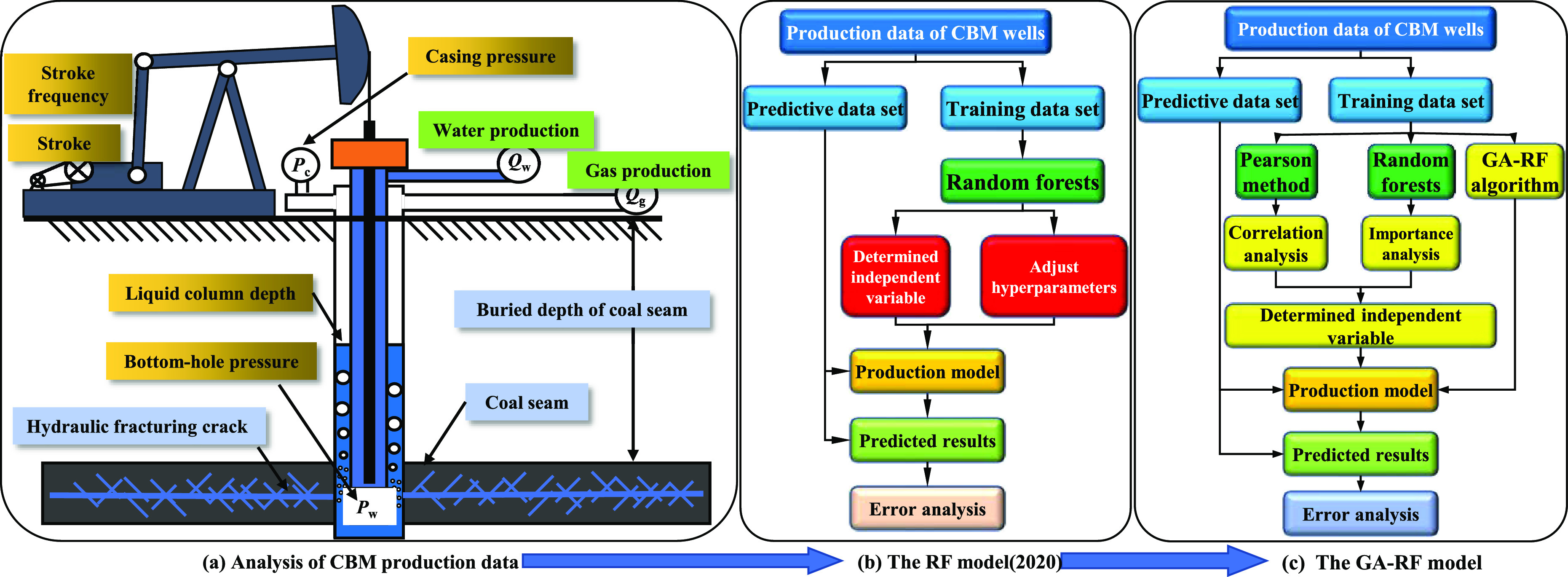
Problems and improvement of the RF model for CBM production.
To avoid the correlated independent variables in the model, the Pearson method and RF were applied to analyze the correlation of production control parameters, and the independent variables influencing gas production were chosen. After determining the independent variables, the RF model optimized by a genetic algorithm (GA) was constructed to automatically adjust its two important hyperparameters, ntree and mtry; then, the optimal hyperparameters were determined. Based on the hybrid GA–RF algorithm, a production model of CBM wells was presented, which showed high accuracy on the production prediction of CBM wells in Qinshui Basin, China.
2. Principle of GA–RF Algorithm
2.1. Random Forests
RF, proposed by Breiman,40 are composed of multiple decision tree models. When a prediction is conducted, multiple decision trees are used to make a joint prediction, ensuring a high-accurate result. The calculation process of a decision tree is shown in Figure 2. When constructing the decision tree, the decision features of internal nodes are selected according to the information gain of the features.
Figure 2.

Calculation process of the decision tree algorithm.
RF include two random steps:
-
(1)
By using the bootstrap method, the original training data are randomly selected as training samples.
-
(2)
Some features can be selected randomly from all features to build a decision tree.
The above data-processing procedures of RF can greatly reduce the correlation between decision trees and further improve the prediction accuracy.
In software programming, RF modeling can determine two important hyperparameters: mtry and ntree. mtry is the number of variables used in the preselection of tree nodes. If the mtry value is too small, it would lead to overfitting (the model is so close to the distribution of training data that it loses the accuracy of prediction) of RF. If it is too large, it would lower the computation speed. ntree is the number of decision trees established by RF. If the values are small, it would cause insufficient training. If the values are large, it would increase the computational complexity of the model and overfitting.
In previous studies,39,41 when establishing the CBM well production prediction model based on RF, the determination of hyperparameter values is manually selected when the error result is small after multiple calculations, causing some problems (especially in the determination of ntree), such as cumbersome multiple calculations and complexity in dealing with multiple CBM well data. Artificial selection may decrease the accuracy of nonoptimal values, so the accuracy of the model needs to be improved. Further, the universality is poor.
RF are suitable to deal with the nonlinear feature calculation. However, the prediction range of the RF is constrained by the highest and lowest sample values in the training data. The prediction results out of the range of the training data may be inaccurate because the prediction range of RF is constrained by the highest and lowest values of the training data.42 Therefore, RF can only predict the production in stages if the data of CBM wells have been analyzed and divided into various stages properly.
2.2. Genetic Algorithm
In order to solve the problems mentioned in Section 2.1 and preferably apply the algorithm to the production fitting and prediction of different CBM wells, GA has been introduced to optimize RF, enabling it to adaptively deal with different CBM well production data and obtain the optimal hyperparameters.
GA is also called evolutionary algorithm, proposed by Holland.43 It draws on Darwin’s population evolution theory and genetic evolution theory to achieve the optimal solution of the problem by simulating the natural population elimination and individual genetic variation processes. By simulating the evolution process of organisms, the individuals in the population are continuously selected, crossed, and mutated, so as to search for the optimal solution adaptively in the solution space.
GA uses the probabilistic optimization method, automatically obtains the optimization search space, and adaptively adjusts the search direction. The basic process can be divided into three steps:44 selection of good varieties (fitness proportionate reproduction), crossing, and mutation. The processes of crossing and mutation are shown in Figure 3.
Figure 3.

Schematic diagram of GA crossover and mutation.
2.3. Construction of the GA–RF Algorithm
In order to increase the universality of RF and improve the accuracy of the RF model when dealing with the production data of different CBM wells, the GA model introduced is set as follows:
-
(1)
The SSE (sum of squared errors) of RF calculation results is set as the fitness function and mtry and ntree as unknown variables.
-
(2)
The initial population size is set as 20 and the number of iterations as 100.
-
(3)
The mutation chance is 0.05 and elitism is 4, and the optimal solution of mtry and ntree is finally obtained.
The specific calculation process is shown in Figure 4. Then, the construction of the GA–RF algorithm is carried out. The solution spaces of ntree and mtry are binary-coded. A population is randomly generated in the solution space as the initial solutions to the problem. The initial solutions of ntree and mtry are brought into RF.
Figure 4.

Construction process of the GA–RF algorithm.
Some features and samples randomly with playback are extracted by using the bootstrap method. The overall data set was divided into ntree groups of data sets. Each group of data sets has the same number of features and samples. The training data randomly selected for the training of the decision tree are in the bag; the rest are out of the bag.
According to the information gain of each characteristic Xi of the data in the bag, the order of Xi was arranged from large to small; then, Xi was selected in turn. The SSE of this feature was calculated to obtain the judgment condition.
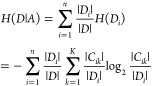
Assuming that the training data set is D, the data set can be divided into Ck (k = 1, 2, 3, ..., K) output variable categories according to different output variables y. A feature A has n different values {a1, a2, a3, ..., an}, and the data set D can be divided into n sets {D1, D2, D3, ..., Dn}. Then, the calculation formula of information gain of feature A is as follows:45
| 1 |
| 2 |
| 3 |
 |
4 |
| 5 |
The information gain g(D, A) of feature A is the difference between the overall empirical entropy H(D) and the conditional empirical entropy H(D|A) of feature A, representing the degree of information complexity (uncertainty) reduction of data set D under the condition of feature A. The larger g(D, A) is, the more important A is to the population D. |D| represents the sample size of the population data set D, and |Ck| represents the sample size of category Ck. |Di| is the sample size of Di, and the sample set belonging to class Ck in subset Di is denoted as Cik, and |Cik| is the sample size of Cik.
Eqs 12345 are used to calculate all the features in the data set and obtain the size of information gain. The feature with the largest information gain is selected as the decision feature of the node, and the node is split according to this feature. After determining the decision feature, by considering the n possible values of this feature in the node, the data in the node are divided into two groups (left child node and right child node). The case where the SSE of the decision tree is the minimum is determined, and the n value is defined as the split condition of the node.
Assuming that the node splits with a certain value ai of feature A, the data points in the node are divided into two groups. The data sample is (n1, n2), and y1® and y2® are the mean values of the output variables of the two groups of data, respectively. In this case, the SSE calculation formula of the decision tree after splitting is as follows:
| 6 |
When the minimum of SSE is determined, the value ai is defined as the splitting decision condition of this node. According to the above steps, the decision features and split conditions of the intermediate nodes of the decision tree are gradually determined. After one of the following two conditions is met, the cycle is stopped. The construction of the decision tree is eventually completed. Using the out-of-bag data to verify the constructed ntree decision trees, the SSE of the RF model is obtained.
-
(1)
The split data set consists of categories of output variables Cik, without feature Xi, which means it is unable to split continually. The modal number of Cik is taken as the leaf node, as shown in result 1 in Figure 2.
-
(2)
For the split data set, the output variables Cik have only one category; meanwhile, the value of Cik is the leaf node, as shown in results 2 and 3 in Figure 2.
The SSE of RF is used as the fitness function to calculate the value of each ntree and mtry individual in the population. The individuals with high fitness are retained; the individuals with low fitness are eliminated. Offspring are generated by crossing the genes of the retained individuals and randomly mutating to increase the genetic diversity, as shown in Figure 3. When the population condition is satisfied, the individual with the highest fitness among all offspring was selected as the optimal solution to the problem.
GA was used to optimize RF, and the optimal value of hyperparameters in RF was determined. The calculation accuracy and error of the algorithm are guaranteed, while the calculation amount of the RF model is reduced.
3. CBM Production Model Based on the GA–RF Algorithm
3.1. Modeling Process
The flowchart of the CBM production model based on the GA–RF algorithm is shown in Figure 5, as follows:
-
①
Analysis of production data: The production data and related parameters of CBM wells were collected. By using RF and the Pearson verification, the importance and correlation of the drainage control parameters were calculated, and the order of parameters affecting the daily production was obtained. The independent variables with high correlation to CBM production were determined.
-
②
Establishment of the GA–RF algorithm: The SSE and hyperparameters of RF were set as the fitness function and unknown variables, respectively, in the GA, and the GA–RF algorithm was established by referring to the algorithm operation flow in Figure 4.
-
③
Training of the GA–RF model: The independent variable parameters were brought into the GA–RF algorithm to establish the production model, and the historical data were used for model training and effectiveness evaluation.
-
④
Model application to CBM production: The model was applied to predict the future production of CBM well after learning and fitting the historical production. The model fitting and prediction results were analyzed to prove the accuracy of the model.
Figure 5.

Establishment of the CBM production model based on the GA–RF algorithm.
Zhu et al.39 and Xue46 collected the drainage and production data of CBM wells in southern Qinshui Basin. The production time is about 2000–3000 days, and the data are recorded once a day. In order to verify the accuracy of the GA–RF model in the fitting and prediction of CBM production, this paper used R language programming to carry out parameter importance analysis and correlation verification for the production data of eight CBM wells in Qinshui Basin. On this basis, the GA–RF model was used to carry out machine learning on the production data of three CBM wells; the fitting and prediction results of the model were obtained as examples to be applied to compare with the actual production data.
3.2. Parameter Importance Analysis
According to the classification standard of CBM wells’ daily production,47 the abovementioned CBM wells can be classified as follows: QN-1 and QN-2 are high-producing wells; QN-3, QN-4, QN-5, QN-6, and QN-7 are medium-producing wells; and QN-8 is a low-producing well. After the site selection, drilling, hydraulic fracturing, and other preliminary works of CBM wells, the drainage parameters during the process of production become the main factors affecting the daily gas production of CBM wells. In this work, we aim to determine the dynamic influence law of the parameters on CBM well production. The parameters of CBM wells include casing pressure, bottom-hole pressure, liquid column depth, stroke frequency, daily gas production, daily decline of casing pressure, and daily decline of bottom-hole pressure.
To understand the significance of the independent variable parameters and ensure whether there is correlation among the parameters affecting the daily gas production of CBM wells, RF were used to calculate the importance of independent variable parameters: supposing ntree decision trees are in the forest, the importance of the features of variable xi calculation formula is:40
| 7 |
where VIMi(Gini) is the importance of feature variable xi; Sxi is the set of all nodes of xi in the ntree decision trees; and Gain (xi, v) is the information gain of xi at node v:40
| 8 |
where vL and vR are the left and right child nodes of node v, respectively; wL and wR are the sample proportion allocated to the left and right child nodes; and GI(v) is the total empirical entropy of node v:40
| 9 |
where pcv is the sample proportion of categories of output variables c in node v, and there are C categories in the output variables.
The production data of CBM wells were input into R language, and the importance analysis was carried out by RF. In the GA–RF model, daily gas production was a dependent variable, whereas casing pressure, bottom-hole pressure, daily decline of casing pressure, daily decline of bottom-hole pressure, liquid column depth, and stroke frequency were independent variables. The importance indexes of the variables are shown in Figure 6.
Figure 6.
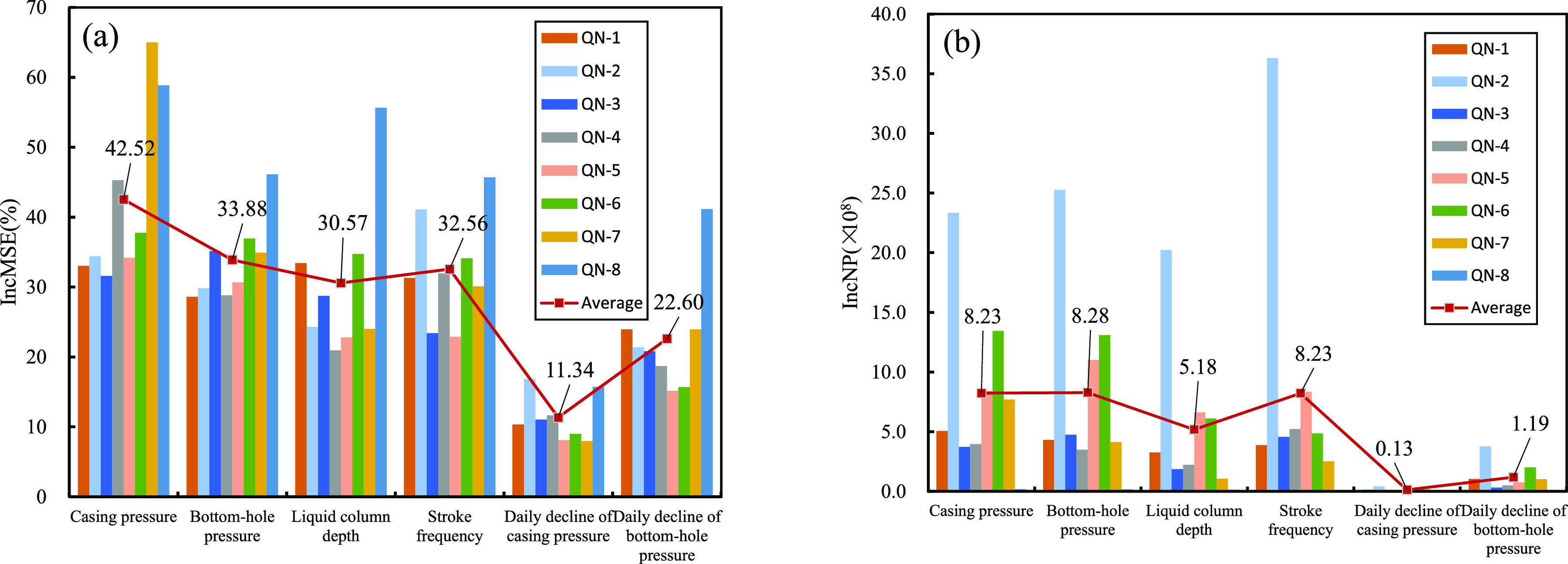
Increment of the parameters MSE and NP. (a) IncMSE for eight CBM wells. (b) IncNP for eight CBM wells.
The increment of mean-square-error (IncMSE) and the increment of node purity (IncNP) were used to estimate the importance of parameters from the perspectives of error increment and information gain, respectively. IncMSE represents the error increment when the feature changes. The greater the value of IncMSE of features xi is, the higher the importance of xi is to the dependent variable (daily gas production). According to the field data of eight CBM wells, IncMSEs of the variables from the largest to the smallest were casing pressure, bottom-hole pressure, stroke frequency, liquid column depth, daily decline of bottom-hole pressure, and daily decline of casing pressure. IncNP represents the information gain of features, which mainly reflects the result of feature selection when the model establishes the decision tree. The greater the IncNP value of xi is, the greater is information content xi carries with the system. IncNPs of the variables from the largest to smallest were casing pressure, bottom-hole pressure, stroke frequency, liquid column depth, daily decline of bottom-hole pressure, and daily decline of casing pressure.
According to the results in Figure 6, the importance order of independent variables from the largest to smallest for the eight CBM wells is as follows: casing pressure, bottom-hole pressure, stroke frequency, liquid column depth, daily decline of bottom-hole pressure, daily decline of casing pressure. For the same CBM well, coal seam depth and hydraulic fracturing properties are invariable, so the correlation with daily gas production is not obvious. Thus, the influence of these static parameters cannot be considered in a single well condition. However, for different CBM wells, there are great differences in stress distribution, permeability, and porosity of coal reservoirs with different depths, leading to changes in production,48,49 and the influence of static parameters such as geological parameters should be considered.
3.3. Correlation Analysis between Drainage Parameters
If the correlation between the parameters of independent variables is high, it will lead to multicollinearity in the process of machine learning, making the estimation of machine learning algorithm invalid and leading to the labeling error’s inaccuracy. Pearson’s verification was used to calculate the correlation among casing pressure, bottom-hole pressure, stroke frequency, liquid column depth, daily decline of bottom-hole pressure, daily decline of casing pressure, and daily gas production. The Pearson verification method is a statistical method, which can quantitatively estimate the correlation between variables. In terms of parameter statistics, this method proved effective.50,51 In computer linguistics, the method is also widely used, mainly for information extraction and other aspects, to calculate the distance between two data and get the similarity. Then, the sets are classified and further studied.
The calculation formula of the Pearson correlation coefficient is as follows:52
| 10 |
where the variables Xi and Yi are the set of x and y coordinates of all points, respectively, and X̅ and Y̅ are the mean values of the x and y coordinates of all points, respectively. Taking QN-8 well as an example, the Pearson verification method was used to obtain the correlation coefficients among various parameters.
When the Pearson method is used to analyze a data set, it is suggested to include at least 30 different samples and at least three variables.53
As shown in Figure 7, casing pressure, bottom-hole pressure, and stroke frequency have higher correlation with daily gas production. Casing pressure and bottom-hole pressure have negative correlation with daily gas production, with the correlation coefficients of −0.23 and −0.19, respectively; stroke frequency is positively correlated with the daily gas production, with the correlation coefficient of 0.19. According to the Pearson verification results, liquid column depth, daily decline of casing pressure, and daily decline of bottom-hole pressure are less correlated with the daily gas production, the correlation coefficients of which are −0.02, 0.05, and 0.09, respectively.
Figure 7.

Correlation of QN-8 well features.
According to the actual production process, after the drilling of CBM wells, hydraulic fracturing is needed, causing more water in the coal reservoir and larger pore pressure, which leads to higher initial flowing pressure and dynamic liquid level. As the drainage works, the bottom-hole pressure, liquid column depth, and pore pressure in the coal reservoir gradually decrease, which leads to the desorption of CBM and the increase of gas production. In the early production stage of CBM wells, the process of holding casing pressure leads to a high casing pressure. With drainage going on, the daily gas production gradually increases and the casing pressure gradually decreases. In the stable drainage stage, the pumping unit stroke increases, which reduces the coal reservoir pressure, enhances gas desorption in coal reservoirs, and improves gas production. According to the calculation in Figure 7, the correlation order of daily gas production from the largest to smallest is as follows: casing pressure, bottom-hole pressure, stroke frequency, daily decline of bottom-hole pressure, daily decline of casing pressure, and liquid column depth.
According to correlation analysis among the process parameters, the bottom-hole pressure is the most correlated with casing pressure, with a coefficient of 0.96. The correlation coefficients between bottom-hole pressure, casing pressure, and stroke frequency are −0.49 and −0.53, respectively.
In Figure 7, the bottom-hole pressure and casing pressure are highly positively correlated, which corresponds to the actual situation. Stroke frequency controls daily water production, which will indirectly affect the casing pressure and bottom-hole pressure. The increase in stroke frequency will lead to an increase in water production and a decrease in bottom-hole pressure, showing a negative correlation with bottom-hole pressure. The increase of stroke frequency leads to the enhancement of gas desorption in coal reservoirs. Theoretically, more desorption gas into the casing will increase casing pressure, but casing pressure is manually reduced to enhance gas production at the scene. Therefore, the actual trend of stroke frequency and casing pressure is opposite, showing a negative correlation.
In summary, the correlation between the parameters obtained by the Pearson verification method is consistent with the actual situation. The correlation between casing pressure and bottom-hole pressure is relatively high. Considering that the actual production is mainly controlled by changing the bottom-hole pressure, the casing pressure parameter is removed from the final independent variable parameters to avoid the occurrence of multicollinearity in the process of machine learning. The correlation between other process parameters (independent variables) is low; so, they are defined as independent variable parameters of CBM production model based on the GA–RF algorithm.
4. Application of Model
4.1. Optimization Results
After the importance and correlation analysis of the in situ parameters, the bottom-hole pressure, stroke frequency, liquid column depth, daily decline of bottom-hole pressure, and casing pressure were defined as independent variables, and daily gas production was taken as a dependent variable. Then, the production model of CBM wells based on the GA–RF algorithm was established. In R program, RF default to mtry = 2 and ntree = 500. In order to improve the calculation accuracy, it is necessary to determine the optimal values of mtry and ntree first. GA is used to optimize RF, which ensures the model’s function of adaptively dealing with different CBM well data and the high accuracy of the model.
Compared with the results of the RF production model,39 the accuracy of the GA–RF model improved effectively, as shown in Figure 8. MSE is also observed to greatly decrease. In R-square (RSQ), the numerical value has also improved slightly, though the original RSQ was high. The specific data of the optimization results are shown in Table 1.
Figure 8.

MSE and RSQ calculated by RF and GA–RF algorithms. (a) MSE calculated by RF and GA–RF algorithms for eight CBM wells. (b) RSQ calculated by RF and GA–RF algorithms for eight CBM wells.
Table 1. Error Analysis of the RF and GA–RF Algorithms.
| well number | RF |
GA–RF |
||||
|---|---|---|---|---|---|---|
| MSE | RSQ | MSE | RSQ | mtry | ntree | |
| QN-1 | 15,596 | 0.9804 | 10,619 | 0.9867 | 2 | 210 |
| QN-2 | 170,192 | 0.9633 | 44,192 | 0.9905 | 3 | 231 |
| QN-3 | 15,356 | 0.9769 | 7496 | 0.9887 | 4 | 290 |
| QN-4 | 11,548 | 0.9820 | 4798 | 0.9925 | 5 | 312 |
| QN-5 | 23,665 | 0.9846 | 12,563 | 0.9918 | 3 | 276 |
| QN-6 | 30,517 | 0.9815 | 10,795 | 0.9934 | 3 | 66 |
| QN-7 | 17,378 | 0.9750 | 9786 | 0.9859 | 3 | 274 |
| QN-8 | 4846 | 0.8634 | 3744 | 0.8929 | 3 | 274 |
The established GA–RF model can adaptively obtain the optimal results of mtry and ntree for different types of CBM well data. mtry can automatically select the optimal value according to the production data of different CBM wells. ntree is significantly reduced after GA optimization; meanwhile, the fitting accuracy of the GA–RF algorithm is significantly improved compared with RF. In terms of MSE reduction, QN-2 well has the largest reduction, with a value of 74.03%. The MSE of other wells is mainly reduced by 40∼60%. R2 increases in QN-8 and QN-2 wells are higher than that in the other wells, and the values are 2.95 and 2.72%, respectively. R2 in the remaining wells increases by about 1%.
Based on the RF production model, the error contours with different ntree and mtry of three CBM wells are shown in Figure 9. For QN-1 and QN-7 wells, MSE decreases with the increase of mtry and ntree. However, for the QN-8 well, MSE decreases first and then goes up when mtry > 3. It is seen that MSE of various CBM wells has a different trend with the change of mtry. For RF, the optimization procedure of ntree and mtry may be less efficient if the hyperparameters of different production types need to be manually selected.
Figure 9.

Error contour of (a) QN-1 (high-yield well), (b) QN-7 (middle-yield well), and (c) QN-8 (low-yield well) by the RF production model.
It can be found that when the GA–RF model was used to calculate the production of different types of CBM wells, it can adjust its own hyperparameters adaptively and directly apply them to calculate without complicated manual operations. The model can obtain the appropriate mtry value, reduce the ntree value to avoid the occurrence of the overfitting phenomenon, reduce the calculation amount of the model, and ensure the accuracy.
4.2. CBM Production Prediction
Through R language, historical data are learned and fitted by using the GA–RF model, and the daily gas production of different types of CBM wells in the next 180 days is predicted to further verify the applicability of the model. Among the three CBM wells, QN-1 well is a high-yield well; QN-7 well is a middle-yield well; and QN-8 well is a low-yield well. As for the different types of CBM wells, the influence relationship of production factors can be obtained from the in situ data, and the results of CBM production prediction based on the GA–RF model are shown in Figure 10.
Figure 10.

Actual and calculated results of (a) QN-1 (high-yield well), (b) QN-7 (middle-yield well), and (c) QN-8 (low-yield well) by the GA–RF production model.
In the training process of the GA–RF model, the fitting relative errors at the initial stage are higher than those at the stable stage. The main reason may be as follows:
-
①
Due to the long time interval of recording production data at the early drainage stage, there are some vacancies in the production data. The main method of dealing with vacancies is through linear completion. This way of filling vacancies will lead to some differences between the supplement and actual data, which eventually affect the fitting accuracy of the model.
-
②
At the initial stage of drainage and production, there are some fluctuations in the CBM production data, such as that in the QN-8 well in Figure 10. It shows that the gas production of CBM wells at the initial stage is unstable, directly leading to the vague connotation relationship between gas production data and drainage parameters, which reduces the model calculation accuracy. When the drainage data at an early stage is relatively smooth, such as that in the QN-7 well in Figure 10, the relative errors more than 10% in the early drainage stage are few.
The results of QN-7 and QN-8 calculated by the production model are closer to the actual data because the previous gas production curves are smoother than that of other CBM wells. Most of the prediction errors of these two wells are less than 10%. Apart from the initial stage, most of the calculated results of QN-1 are close to the actual data curve because there are obvious fluctuations in the initial stage. The existence of the interpumping operation, pumping unit efficiency reduction, pumping unit maintenance, and so on leads to the deviation of the production model calculation results, but 79.44% of the prediction errors are still below 10%.
The GA–RF model for predicting CBM production has satisfied the calculation accuracy. The results of standard deviation (SD), root-mean-square error (RMSE), absolute average relative deviation (AARD), and average relative deviation (ARD) are listed in Table 2. Min. of ARD and Max. of ARD (%) refer to minimum and maximum absolute relative deviation values, respectively. The error functions in Table 2 were calculated by the following equations:54
| 11 |
| 12 |
| 13 |
| 14 |
Table 2. Error Parameters of the Model.
| well number | data set | SD | RMSE | AARD (%) | ARD (%) | min. of ARD (%) | max. of ARD (%) |
|---|---|---|---|---|---|---|---|
| QN-1 | training | 0.225 | 52.421 | 2.491 | –1.546 | 0.001 | 60.389 |
| test | 0.069 | 202.856 | 5.300 | –4.232 | 0.036 | 15.346 | |
| total | 0.217 | 75.021 | 2.702 | –1.748 | 0.001 | 60.389 | |
| QN-7 | training | 0.065 | 54.415 | 1.365 | –0.275 | 0.001 | 36.107 |
| test | 0.049 | 105.425 | 4.054 | –3.181 | 0.016 | 11.372 | |
| total | 0.064 | 59.450 | 1.554 | –0.479 | 0.001 | 36.107 | |
| QN-8 | training | 0.070 | 29.205 | 2.508 | –0.576 | 0.001 | 55.459 |
| test | 0.070 | 37.032 | 5.751 | –1.867 | 0.076 | 27.874 | |
| total | 0.070 | 29.891 | 2.762 | –0.677 | 0.001 | 55.459 |
For QN-1, QN-7, and QN-8, the prediction results of the GA–RF model are accepted. The maximum AARD of training data, test data, and total data are 2.508, 5.751, and 2.762%, respectively. The maximum RMSE of training data, test data, and total data are 54.415, 202.856, and 75.021, respectively.
The error frequency of the GA–RF model is shown in Figure 11. When the absolute relative error is 15%, the cumulative error frequencies in the training and prediction periods of QN-1, QN-7, and QN-8 calculated by the model are 98.38, 99.55, 98.25% and 79.44, 99.44, 86.67%, respectively. In the training period, 98% of the errors are less than or equal to 15%, and 88% of the prediction errors are less than or equal to 15%. Hence, the GA–RF model has satisfied the calculation accuracy.
Figure 11.

Relative error frequency and cumulative frequency of (a) QN-1, (b) QN-7, and (c) QN-8 by the GA–RF production model.
Considering that CBM production is time-related, the calculation errors of the production model change in different production stages, which decreases the prediction accuracy of the model. Therefore, locally estimated scatterplot smoothing (LOESS) method was used to conduct outlier analysis on the errors of the GA–RF model to take the influence of time series into account to smoothen the scatters. The error curves of QN-1, QN-7, and QN-8 were calculated, as shown in the black curves in Figure 12. The upper limit of error outlier determination was set with fivefold SDs plus the LOESS curve, and the error higher than this limit will be considered as an outlier, as shown in the red curve in Figure 12. Most of the error outliers are concentrated at the initial stage of training. There are also some error outliers of QN-1 and QN-8 prediction stages. According to statistics, there are 138 outliers in 2400 data samples of QN-1, 119 outliers in 2560 data samples of QN-7, and 212 outliers in 2300 data samples of QN-8, accounting for 6, 5, and 9% errors, respectively. It means that the model is stable in calculation accuracy.
Figure 12.

Error outliers of (a) QN-1, (b) QN-7, and (c) QN-8 by the GA–RF production model.
The model shows good performance in the fitting and prediction of CBM production, which provides a reference for the production prediction of the CBM wells. Based on the GA–RF production model trained by the historical production data, the coincidence degree between the fitting curve and the actual production curve is high, and the relative errors in 93% of fitting results are less than 5%. After training, the model can perform production prediction using the production parameters. The relative errors in 89% of predictions are less than 10%. When there are no (or few) anomalies in CBM wells, the accuracy of prediction results may improve a lot. When volatility anomaly occurs, the calculation results of the model in the abnormal part would deviate. Therefore, when using this GA–RF model to predict the daily gas production of CBM wells, it is necessary to analyze the production data and handle the abnormal data appropriately, which is an important step to ensure the production prediction validity of the GA–RF production model.
5. Conclusions
RF have been optimized by GA to increase the efficiency of hyperparameter determination because the GA–RF algorithm can automatically adjust the algorithm to achieve the optimal hyperparameters. Compared with RF, the MSE of the GA–RF algorithm is reduced by 40–60%. The value of the determination parameter, R2, goes up to about 1%.
The importance and correlation indexes of CBM production data have been calculated by the GA–RF algorithm. The results show that casing pressure, bottom-hole pressure, and stroke frequency should be emphasized in the drainage control process because the parameters have important effects on the daily gas production of CBM wells.
A CBM production model based on the GA–RF algorithm was presented to analyze the daily gas production of CBM wells with different production capacities at Qinshui Basin in China. The results of the model are in good agreement with the actual production because 93% of the calculated relative errors are less than 5%. For gas production prediction, 89% of the relative errors are less than 10%. The error sets of the CBM production model have error outliers with 5–9%. This indicates that the model based on the GA–RF algorithm can provide high precision results for predicting CBM production.
Acknowledgments
This research was supported by the National Nature Science Foundation of China (52074297) and the Central University Basic Research Fund of China (2021YJSLJ02).
The authors declare no competing financial interest.
References
- Clarkson C. R.; Qanbari F. A Semi-Analytical Method for Forecasting Wells Completed in Low Permeability, Undersaturated CBM Reservoirs. J. Nat. Gas Sci. Eng. 2016, 30, 19–27. 10.1016/j.jngse.2016.01.040. [DOI] [Google Scholar]
- Ju W.; Jiang B.; Qin Y.; Wu C.; Li M.; Xu H.; Wang S. Characteristics of Present-day In-situ Stress Field Under Multi-seam Conditions: Implications for Coalbed Methane Development. J. China Coal Soc. 2020, 45, 3492–3500. [Google Scholar]
- Karacan C. O.; Ruiz F. A.; Cote M.; Phipps S. Coal Mine Methane: A Review of Capture and Utilization Practices with Benefits to Mining Safety and to Greenhouse Gas Reduction. Int. J. Coal Geol. 2011, 86, 121–156. 10.1016/j.coal.2011.02.009. [DOI] [Google Scholar]
- Flores R. M.; Rice C. A.; Stricker G. D.; Warden A. Methanogenic Pathways of Coal-bed Gas in the Powder River Basin, United States: The Geologic Factor. Int. J. Coal Geol. 2008, 76, 52–75. 10.1016/j.coal.2008.02.005. [DOI] [Google Scholar]
- Guo C.; Xia Y.; Ma D.; Sun X.; Dai G.; Shen J.; Chen Y.; Lu L. Geological Conditions of Coalbed Methane Accumulation in the Hancheng Area, Southeastern Ordos Basin, China: Implications for Coalbed Methane High-yield Potential. Energy Explor. Exploit. 2019, 37, 922–944. 10.1177/0144598719838117. [DOI] [Google Scholar]
- Li S.; Tang D.; Pan Z.; Xu H.; Tao S.; Liu Y.; Ren P. Geological Conditions of Deep Coalbed Methane in the Eastern Margin of the Ordos Basin, China: Implications for Coalbed Methane Development. J. Nat. Gas Sci. Eng. 2018, 53, 394–402. 10.1016/j.jngse.2018.03.016. [DOI] [Google Scholar]
- Scott A. R. Hydrogeologic Factors Affecting Gas Content Distribution in Coal Beds. Int. J. Coal Geol. 2002, 50, 363–387. 10.1016/S0166-5162(02)00135-0. [DOI] [Google Scholar]
- Voast V.; Wayne A. Geochemical Signature of Formation Waters Associated with Coalbed Methane. Am. Assoc. Pet. Geol. Bull. 2003, 87, 667–676. 10.1306/10300201079. [DOI] [Google Scholar]
- Yao Y.; Liu D.; Yan T. Geological and Hydrogeological Controls on the Accumulation of Coalbed Methane in the Weibei Field, Southeastern Ordos Basin. Int. J. Coal Geol. 2014, 121, 148–159. 10.1016/j.coal.2013.11.006. [DOI] [Google Scholar]
- Zhang S.; Zhang X.; Li G.; Liu X.; Zhang P. Distribution Characteristics and Geochemistry Mechanisms of Carbon Isotope of Coalbed Methane in Central-southern Qinshui basin. China. Fuel 2019, 244, 1–12. 10.1016/j.fuel.2019.01.129. [DOI] [Google Scholar]
- Li X.; Wang Y.; Jiang Z.; Chen Z.; Wang L.; Wu Q. Progress and Study on Exploration and Production for Deep Coalbed Methane. J. China Coal Soc. 2016, 41, 24–31. [Google Scholar]
- Kumar H.; Elsworth D.; Liu J.; Pone D.; Mathews J. P. Optimizing Enhanced Coalbed Methane Recovery for Unhindered Production and CO2 Injectivity. Int. J. Greenhouse Gas Control 2012, 11, 86–97. 10.1016/j.ijggc.2012.07.028. [DOI] [Google Scholar]
- Sun Z.; Huang B.; Li Y.; Lin H.; Shi S.; Yu W. Nanoconfined Methane Flow Behavior through Realistic Organic Shale Matrix under Displacement Pressure: a Molecular Simulation Investigation. J. Pet. Explor. Prod. Technol. 2021, 12, 1193–1201. 10.1007/s13202-021-01382-0. [DOI] [Google Scholar]
- Cen X.; Wu X.; Liang W.; Li S.; Tang X.; You Q.; Zheng F. Analysis of Factors Affecting Productivity of Coalbed Gas Wells. Sci. Technol. Eng. 2014, 14, 201–204. [Google Scholar]
- Bowers C. E.Analyzing Fracture Stimulation of Middle Devonian Strata in Clearfield County Pennsylvania Using a 3D Geomechanical Fault Model and Microseismic. M.S. Thesis, West Virginia University, 2014.
- Shaw D.; Mostaghimi P.; Armstrong R. T. The Dynamic Behaviour of Coal Relative Permeability Curves. Fuel 2019, 253, 293–304. 10.1016/j.fuel.2019.04.107. [DOI] [Google Scholar]
- Han X.; Yang J. Coalbed Methane Deliverability Characteristic and Its Controlling Factors in Southern Qinshui Basin. Sci. Technol. Eng. 2013, 13, 9940–9945. [Google Scholar]
- Ren J.; Ren S.; Meng S. Analysis of Production Rule and Productivity Influencing Factors of Coalbed Methane. Sci. Technol. Eng. 2013, 13, 2799–2802. [Google Scholar]
- Bakhshi E.; Golsanami N.; Chen L. Numerical Modeling and Lattice Method for Characterizing Hydraulic Fracture Propagation: A Review of the Numerical, Experimental, and Field Studies. Arch. Comput. Methods Eng. 2020, 28, 3329–3360. 10.1007/s11831-020-09501-6. [DOI] [Google Scholar]
- Zhu J.; Tang J.; Hou C.; Shao T.; Zhao Y.; Wang J.; Lin L.; Liu J.; Jiang Y. Two-phase Flow Model of Coalbed Methane Extraction with Different Permeability Evolutions for Hydraulic Fractures and Coal Reservoirs. Energy Fuels 2021, 35, 9278–9293. 10.1021/acs.energyfuels.1c00404. [DOI] [Google Scholar]
- Li B.; Yang K.; Ren C.; Li J.; Xu J. An Adsorption-permeability Model of Coal with Slippage Effect Under Stress and Temperature Coupling Condition. J. Nat. Gas Sci. Eng. 2019, 71, 102983 10.1016/j.jngse.2019.102983. [DOI] [Google Scholar]
- Sun Z.; Shi J.; Wu K.; Tao Z.; Feng D.; Li X. Effect of Pressure-Propagation Behavior on Production Performance: Implication for Advancing Low-Permeability Coalbed-Methane Recovery. SPE J. 2018, 24, 681–697. 10.2118/194021-PA. [DOI] [Google Scholar]
- Sun Z.; Huang B.; Wu K.; Shi S.; Wu Z.; Hou M.; Wang H. Nanoconfined Methane Density Over Pressure and Temperature: Wettability Effect. J. Nat. Gas Sci. Eng. 2022, 99, 104426 10.1016/j.jngse.2022.104426. [DOI] [Google Scholar]
- Maxwell K.; Rajabi M.; Esterle J. Automated Classification of Metamorphosed Coal from Geophysical Log Data Using Supervised Machine Learning Techniques. Int. J. Coal Geol. 2019, 214, 103284 10.1016/j.coal.2019.103284. [DOI] [Google Scholar]
- Lolon L.; Hamideh K.; Weijers L.; Mayerhofer M.; Melcher H.; Oduba O.. Evaluating the Relationship between Well Parameters and Production Using Multivariate Statistical Models: a Middle Bakken and Three Forks Case History; SPE Hydraulic Fracturing Technology Conference; Woodlands, Texas, USA; 2016. [Google Scholar]
- Chattaraj S.; Mohanty D.; Kumar T.; Halder G.; Mishra K. Comparative Study on Sorption Characteristics of Coal Seams from Barakar and Raniganj Formations of Damodar Valley Basin, India. Int. J. Coal Geol. 2019, 212, 103202. 10.1016/j.coal.2019.05.009. [DOI] [Google Scholar]
- Al-Anazi A.; Gates I. D. A Support Vector Machine Algorithm to Classify Lithofacies and Model Permeability in Heterogeneous Reservoirs. Eng. Geol. 2010, 114, 267–277. 10.1016/j.enggeo.2010.05.005. [DOI] [Google Scholar]
- Corina A. N.; Hovda S. Automatic Lithology Prediction from Well Logging Using Kernel Density Estimation. J. Pet. Sci. Eng. 2018, 170, 664–674. 10.1016/j.petrol.2018.06.012. [DOI] [Google Scholar]
- Shuvajit B.; Timothy R. C.; Mahesh P. Comparison of Supervised and Unsupervised Approaches for Mudstone Lithofacies Classification: Case Studies from the Bakken and Mahantango-Marcellus Shale, USA. J. Nat. Gas Sci. Eng. 2016, 33, 1119–1133. 10.1016/j.jngse.2016.04.055. [DOI] [Google Scholar]
- Gu Y.; Bao Z.; Rui Z. Complex Lithofacies Identification Using Improved Probabilistic Neural Networks. Petrophysics 2018, 59, 245–267. 10.30632/PJV59N2-2018a9. [DOI] [Google Scholar]
- Xie Y.; Zhu C.; Zhou W.; Li Z.; Liu X.; Tu M. Evaluation of Machine Learning Methods for Formation Lithology Identification: A Comparison of Tuning Processes and Model Performances. J. Pet. Sci. Eng. 2018, 160, 182–193. 10.1016/j.petrol.2017.10.028. [DOI] [Google Scholar]
- Xu X.; Rui X.; Fan Y.; Yu T.; Ju Y. A Multivariate Long Short-Term Memory Neural Network for Coalbed Methane Production Forecasting. Symmetry 2020, 12, 2045. 10.3390/sym12122045. [DOI] [Google Scholar]
- Xu X.; Rui X.; Fan Y.; Yu T.; Ju Y. Forecasting of Coalbed Methane Daily Production Based on T-LSTM Neural Networks. Symmetry 2020, 12, 861. 10.3390/sym12050861. [DOI] [Google Scholar]
- Mahdaviara M.; Rostami A.; Keivanimehr F.; Shahbazi K. Accurate Determination of Permeability in Carbonate Reservoirs Using Gaussian Process Regression. J. Pet. Sci. Eng. 2021, 196, 107807 10.1016/j.petrol.2020.107807. [DOI] [Google Scholar]
- Rostami A.; Baghban A. Application of a Supervised Learning Machine for Accurate Prognostication of Higher Heating Values of Solid Wastes. Energy Sources, Part A 2018, 40, 558–564. 10.1080/15567036.2017.1360967. [DOI] [Google Scholar]
- Rostami A.; Kamari A.; Panacharoensawad E.; Hashemi A. New Empirical Correlations for Determination of Minimum Miscibility Pressure (MMP) during N2-contaminated Lean Gas Flooding. J. Taiwan Inst. Chem. Eng. 2018, 91, 369–382. [Google Scholar]
- Rostami A.; Arabloo M.; Esmaeilzadeh S.; Mohammadi A. H. On Modeling of Bitumen/n-tetradecane Mixture Viscosity: Application in Solvent-assisted Recovery Method. Asia-Pac. J. Chem. Eng. 2017, 13, e2152 10.1002/apj.2152. [DOI] [Google Scholar]
- Lu Y.; Tang D.; Li Z.; Shao X.; Xu H. Fitting and Predicting Models for Coalbed Methane Wells Dynamic Productivity. J. China Coal Soc. 2011, 36, 1481–1485. [Google Scholar]
- Zhu Q.; Hu Q.; Du H.; Fan B.; Zhu J.; Zhang B.; Zhao Y.; Liu B.; Tang J. A Gas Production Model of Vertical Coalbed Methane Well Based on Random Forest Algorithm. J. China Coal Soc. 2020, 45, 2846–2855. [Google Scholar]
- Breiman L. Random Forests. Machine Learning 2001, 45, 5–32. 10.1023/A:1010933404324. [DOI] [Google Scholar]
- Chen Y.; Mao Y. Automatic Tuning of Ceph Parameters Based on Random Forest and Genetic Algorithm. J. Comput. Appl. 2020, 40, 347–351. [Google Scholar]
- Tsuchiya M.; Yamauchi Y.; Yamashita T.; Fujiyoshi H.. Transfer Forests Based on Covariate Shift. 2015 3rd IAPR Asian Conference on Pattern Recognition (ACPR); IEEE, 2015; pp 760–764. [Google Scholar]
- Holland J. H.Adaption in Natural and Artificial Systems. University of Michigan Press:Michigan, 1975. [Google Scholar]
- De Jong K. Adaptive System Design: A Genetic Approach. IEEE Trans. Syst. Man, Cybern. 1980, 10, 566–574. 10.1109/TSMC.1980.4308561. [DOI] [Google Scholar]
- Shannon C. E.; Weaver W. The Mathematical Theory of Communication. Philos. Rev. 1949, 60, 398–400. 10.2307/2181879. [DOI] [Google Scholar]
- Xue D.Research on the Relationship of Drainage Parameters in CBM Wells Based on Big Data Analysis. M.S. Thesis. China University of Petroleum: Beijing, 2019.
- Zhao X.; Yang Y.; Chen L.; Yang Y.; Shen J.; Chao W.; Shao G. Production Controlling Mechanism and Mode of Solid-fluid Coupling of High Rank Coal Reservoirs. Acta Pet. Sin. 2015, 36, 1029–1034. 10.7623/syxb201509001. [DOI] [Google Scholar]
- Qin Y.; Shen J. On the Fundamental Issues of Deep Coalbed Methane Geology. Acta Pet. Sin. 2016, 37, 125–136. [Google Scholar]
- Ye J.; Zhang S.; Ling B.; Zheng G.; Wu J.; Li D. Study on Variation Law of Coalbed Methane Physical Property Parameters with Seam Depth. Coal Sci. Technol. 2014, 42, 35–39. [Google Scholar]
- Cho S. J.; Li F.; Bandalos D. Accuracy of the Parallel Analysis Procedure with Polychoric Correlations. Educ. Psychol. Meas. 2009, 69, 748–759. 10.1177/0013164409332229. [DOI] [Google Scholar]
- Teng W.; Cheng L.; Zhao K.. Application of Kernel Principal Component and Pearson Correlation Coefficient in Prediction of Mine Pressure Failure. 2017 Chinese Automation Congress (CAC); IEEE, 2017. [Google Scholar]
- Rodgers L.; Nicewander W. A. Thirteen Ways to Look at the Correlation Coefficient. Am. Stat. 1988, 42, 59–66. 10.2307/2685263. [DOI] [Google Scholar]
- Koo T. K.; Li M. Y. A Guideline of Selecting and Reporting Intraclass Correlation Coefficients for Reliability Research. J. Chiropr. Med. 2016, 15, 155–163. 10.1016/j.jcm.2016.02.012. [DOI] [PMC free article] [PubMed] [Google Scholar]
- Mahdaviara M.; Rostami A.; Shahbazi K. Smart Learning Strategy for Predicting Viscoelastic Surfactant (VES) Viscosity in Oil Well Matrix Acidizing Process Using a Rigorous Mathematical Approach. SN Appl. Sci. 2021, 3, 815. 10.1007/s42452-021-04799-8. [DOI] [Google Scholar]