Impact of minimal sufficient balance, minimization, and stratified permuted blocks on bias and power in the estimation of treatment effect in sequential clinical trials with a binary endpoint

Abstract

Minimization is among the most common methods for controlling baseline covariate imbalance at the randomization phase of clinical trials. Previous studies have found that minimization does not preserve allocation randomness as well as other methods, such as minimal sufficient balance, making it more vulnerable to allocation predictability and selection bias. Additionally, minimization has been shown in simulation studies to inadequately control serious covariate imbalances when modest biased coin probabilities (≤0.65) are used. This current study extends the investigation of randomization methods to the analysis phase, comparing the impact of treatment allocation methods on power and bias in estimating treatment effects on a binary outcome using logistic regression. Power and bias in the estimation of treatment effect was found to be comparable across complete randomization, minimization, and minimal sufficient balance in unadjusted analyses. Further, minimal sufficient balance was found to have the most modest impact on power and the least bias in covariate-adjusted analyses. The minimal sufficient balance method is recommended for use in clinical trials as an alternative to minimization when covariate-adaptive subject randomization takes place.

1. Introduction and background

Randomization protects the integrity of clinical trials against selection bias and is the basis for sound statistical inference. Moreover, randomization is an indispensable aspect of all empirical trials, making it the gold standard for inferences on efficacy of treatments.^1–7 In clinical trials, assigning patients to treatment arms that have the same spectrum of prognosis allows researchers to isolate the effect of treatment, rather than have results confounded by other important prognostic variables.⁴ Use of complete randomization (also referred to as simple randomization), in which each subject has the exact same probability of being assigned to any of the treatment arms, is waning in practice.² Although in large trials, on average, complete randomization will result in comparable covariate distributions across treatment arms, there is a chance that large imbalances may occur at random. This is magnified in trials with small or medium sample sizes.^3,4,8 Clinical trials with substantial imbalances in important prognostic factors come under criticism, even though they may occur by chance.^3,9 As a result, preventing serious imbalances in known baseline factors is highly desired and has been focused on in recent clinical trials literature.^5,10–14 Although the “Introduction and background” section of this study discusses many of the same topics as Lauzon et al.,¹³ these are included in this study for completeness.

Review of the literature suggests use of covariate information in the randomization phase of clinical trials is on the rise,^15,16 especially in phase III cancer clinical trials. For instance, Pond et al.¹⁷ showed 85% of phase III cancer clinical trials incorporate at least one baseline variable in their randomization. It should be noted, however, not all procedures are equally adept at controlling imbalance across treatment arms.¹⁸ Additionally, flawed balancing procedures may lead to distorted results, indirectly causing real harm to patients.^18,19 Although it is common to indiscriminately use randomization methods that have previously been implemented in clinical trials, investigators deserve complete and balanced information on the capacities and limitations of randomization methods used in clinical trials. These capacities and limitations are measured on both the method’s ability to control covariate imbalance and to allow for reasonable proportions of unconstrained, complete random treatment assignments.⁵

An early solution for controlling covariate imbalance across treatment arms was stratification.⁴ Although there are many variations of stratification, typically it entails forming two or more levels of each known prognostic factor and sorting subjects accordingly. Then randomization of subjects to treatment arms is performed independently within each stratum, preserving the desired allocation within each stratum. “Stratified permuted block randomization to reduce imbalance on known prognostic factors is still commonly used.²⁰ The main drawback of this approach is, number of strata increases geometrically as the number of prognostic variables increases.⁴ As a result, in general, stratified randomization methods tend to be infeasible when there are more than three or four prognostic variables”.²¹

Dynamic allocation methods such as minimization^22,23 and minimal sufficient balance¹² (MSB) offer an alternative to stratification to control imbalance on a large number of prognostic variables.^3,24 Dynamic allocation methods often involves using information from covariates to determine whether a specific treatment arm should be favored, and use either biased coin or deterministic treatment assignments to favor that arm. While regulatory agencies (e.g. FDA, and EMA), state that randomization methods must have a random component, stratified permuted blocks have deterministic treatment assignments for at least the final subject in every block, and this method is most commonly used for subject randomization in clinical trials.^15,16 Thus, alternatives with a greater proportion of completely random treatment assignments are desirable and may be closer to the intent of randomization than commonly used methods.

As an alternative to stratified randomization, Taves²² and Pocock and Simon²³ independently proposed minimization (or more generally known as adaptive stratification). When using minimization, important prognostic factors are identified and continuous variables are categorized before the trial begins. Then, assignment of a new patient to a treatment arm is done using a biased coin to favor an assignment that will minimize the difference between treatment arms in terms of these covariates. Minimization controls imbalance in the treatment distribution within covariate margins associated with the current subjects, as opposed to stratification, which controls imbalance in treatment distribution with the covariate stratum associated with the current subject.²¹ Detailed information on the implementation of minimization can be found in Lauzon et al.,¹³ and Pocock and Simon.²³

In clinical trials literature, stratification with permuted blocks is the most popular method for assigning subjects to treatments when balance is sought in a prognostic, followed by minimization.^15,16 Minimization is gaining popularity in recent years,^3,24 and is often advised for use in clinical trials.^{2,4,22,23,25–27} Statistical arguments in favor of minimization argue that it controls imbalance more effectively than simple randomization and can allow for more covariates than stratification.^4,22,23,27 Comparisons between minimization and other methods of dynamic allocation that control imbalance on several prognostic factors, such as Kuhn et al.¹¹ and Lauzon et al.,¹³ have shown benefits and drawbacks of minimization. Criticisms of minimization primarily point out that minimization attempts to control aggregate imbalances, rather than imbalance in each covariate.²⁸ Another major drawback of minimization is, for continuous covariates, the method is sensitive to the cutoff for stratification set by the clinicians and statisticians prior to the trial.²¹ Those who argue for use of minimization in clinical trials cite its effectiveness of controlling baseline prognostic factors.^5,21,29 However, when continuous covariates are to be balanced on, covariate imbalance is reduced.¹³ Additionally, the impact of the loss in allocation randomness inherent to minimization due to adjustments being made for minor covariates differences across treatment arms has rarely been addressed. Nonetheless, there are a few alternatives to minimization that have been proposed to control imbalance with any number of covariates.^28,30

Zhao, Hill and Palesch¹² proposed MSB as an alternative to minimization. Its purpose is to control serious imbalances and preserve a high level of allocation randomness and it is recommended for use in clinical trials where covariate imbalance is to be controlled in the randomization phase of the trial.^5,12 The MSB method uses biased coin treatment assignments only when at least one covariate imbalance exceeds a pre-specified limit and a biased coin assignment is expected to reduce the imbalance. Covariates whose imbalance crosses the pre-specified threshold result in votes to favor treatment or control groups in order to decrease the imbalance in the covariate. Votes (which may the weighed unequally) are tallied, and the treatment with the most votes is favored using the prespecified fixed biased coin probability. Otherwise, a complete random assignment is applied by default.^5,12 Detailed information on the implementation of MSB, can be found in Lauzon et al.¹³ and Zhao et al.¹²

Zhao et al.¹² using a biased coin probability of 0.65 found, using MSB with a serious imbalance defined as p-value <0.3 from a test of imbalance of each covariate across treatment arms (e.g. t-test, Wilcoxon rank-sum test, Chi-squared test, or Fisher’s exact test), for five baseline covariates (one categorical, 4 continuous) resulted in 58.8% unconstrained randomized assignments.⁵ In Lauzon et al.,¹³ treatment assignments were re-randomized using minimization and MSB and imbalance was controlled on five covariates (four continuous, one categorical), and 11 covariates (eight continuous, three categorical). The data used for re-randomization came from the National Institute of Neurological Disorders and Stroke tissue plasminogen activator study for ischemic stroke.³¹ It was shown that, compared with minimization, MSB performed as well or better at controlling imbalance, and also had a higher degree of allocation randomness, all while preserving the nominal type I error rate for the study. Additionally, the differences in effectiveness at reducing covariate imbalance, for both methods, were greater when imbalance was controlled on a large number of covariates (11) than when imbalance was controlled on a moderate number of covariates (5).

Selection bias, controlling covariate imbalance, and preservation of the nominal type I have been the focus in comparing methods for controlling covariate imbalance.¹³ However, there are other important considerations when making informed decisions about which method to use in a clinical trial. Specifically, maintaining power and unbiasedness in the estimation of treatment effect. Birkett et al.⁴ have considered bias and power in detecting treatment effects for a model with up to four continuous covariates and a continuous outcome for moderate and large samples (more than 100 subjects) and found that minimization and stratification do not bias the treatment effect. However, small sample sizes are common in trials on rare diseases. Moreover, even in large trials, interim analyses are often planned at stages of trials when the sample sizes are not larger than 100. Furthermore, no study has considered the impact of MSB in the analysis phase of a trial. Because binary endpoints are commonly used in clinical trials, they will be the focus of this study, and logistic regression will be used as a model for data analysis.

Many studies describing stratification or minimization do not mention any implications of these in the analysis.^16,32–38 However, when such implications are discussed, most authors recommend adjusting for covariates in the analyses when randomization methods control imbalance on them.^{1,4,21,24,39–44,45–51} The claim is, if variables included in the randomization method are not adjusted for in the analysis, power can be compromised,²⁴ or the type I error rate can be reduced.^4,16,48–51 However, the literature is lacking in head-to-head comparisons of the more complex dynamic allocation methods in terms of bias and power in the estimation of treatment effect.

It is well established that controlling for highly prognostic factors in a regression analysis can lead to statistically significant increases in power to detect treatment effect, compared with cases where those factors are not controlled for.^{15,17,21,23,52–58} In clinical trial data analysis, it is imperative to adjust in the analysis phase for covariates known to influence the primary outcome;^48,59–67 failure to do so could result in inflated type I error rates,^41,59,66 biased treatment effect estimation,^42,59 and loss of power to detect treatment effect.^{52,59,60,63–65,68,69} This study aims to investigate the effects of including covariates in the randomization procedure on both adjusted and unadjusted analyses when using stratified permuted blocks, minimization and MSB methods.

This manuscript investigates properties related to power and bias in the estimation of treatment effect for complete randomized design, stratified permuted blocks, minimization, and MSB methods. In the “Method” and “Results” sections, a simulation study is outlined, and results of the bias and power for inferences on treatment effects with a binary outcome is presented. This will be followed by a discussion in the “Discussion” section.

2. Method

Although alternate versions of minimization exist where, for example, the method for measuring imbalance is changed, or covariate weighting is used,³ in practice Berger²⁸ has found that the minimization of Pocock and Simon²³ is most commonly used and in some applications Taves’s²² minimization (deterministic minimization) is also used.

The conditional probability of assigning a subject to a given treatment can differ according to the method of randomization used. In complete randomization when there are two treatments, the probability of allocation to active treatment is 0.5. When stratification is used for randomization, combinations of strata from each factor create subsets of the data and guarantee perfect (or near perfect) balance on categorical variables. Subjects within each subset have a probability of allocation to the active treatment of 0.5 if they are the first subject in the block. Subsequent subjects would have a probability of assignment to active treatment equal to the number of remaining subjects in the block that are to receive active treatment divided by the total number of subjects remaining in the block.

In the case of minimization and MSB, complete random or biased coin treatment assignments are determined once any covariate imbalances have been identified according to a pre-specified threshold. In the case of deterministic minimization, the first subject in the study is assigned to treatment or control with probability 0.5, and subsequent subjects are assigned to the treatment that minimizes the total imbalance in the covariates. If both treatments result in the same total imbalance in the covariates, the subject is assigned to treatment or control groups with probability 0.5.

The primary goal of this article is to perform a simulation study that compares power and bias for measuring treatment effect across several randomization methods commonly used in the context of covariate balancing. Modeling situations considered vary by sample size, covariate effects, and whether endpoints are adjusted for. For simplicity, only randomization in sequential clinical trials consisting of a treatment with two levels, equal marginal allocation ratios for each treatment, and a binary outcome are considered. More complex modeling, such as a model with five and 11 covariates, has been considered in Lauzon et al.13 The five methods of randomization considered are complete randomization, stratified permuted blocks, minimization with biased coin treatment assignments (referred to as minimization), minimization with deterministic treatment assignments (referred to as deterministic minimization), and MS. In this study, the stratified permuted block method uses a block size of six, which is arbitrarily chosen without loss of generality. In these simulations, relevant metrics were obtained from logistic regression.

2.1. Simulation study

Three sample sizes (n = 50, n = 100, and n = 500) were considered, representing small, moderate, and large sample sizes. Two scenarios were considered for covariates: The first scenario included a random noise covariate, and the second scenario included both a random noise covariate and a potential confounding covariate. In each set of simulations, both covariate-adjusted and unadjusted estimates of treatment effects, and hypothesis tests of treatment effects were performed. In all cases, the treatment variable had an underlying relationship with the binary outcome which resulted in an odds ratio resulting in 80% power to detect a treatment effect at the 0.05-level when no covariates (other than treatment effect) were included in the model. Ten-thousand simulations of each scenario were performed. Because there were three sample sizes considered, four models of covariates, and covariate-adjusted and unadjusted simulations, there were 240,000 simulations studies considered. In addition, to determine the impact of prevalence of the outcome on results, six additional simulation scenarios were considered, resulting in 300,000 total simulation studies considered.

In scenarios where the random noise continuous covariate (distributed as a standard normal variable) is used, it was dichotomized at the median to include in the minimization and stratified permuted blocks methods. The other covariate used in the simulations is a binary covariate with odds ratios for having the outcome of 1.5, 2, or 5. Based on the effects of the intercept, treatment variable, and the covariate variable, for each simulation, the outcome was generated by converting the log-odds of each subject having the outcome to a probability and using a uniform (0, 1) random number generator to assign the subjects to each level of the outcome variable with the appropriate probability. The minimization procedure used follows the procedure of Pocock and Simon²³ with a biased coin probability of 0.65. The deterministic minimization follows the procedure of Taves.²² In the implementation of MSB, serious imbalance is defined as a p-value below 0.3 on a balance test (Chi-Squared Test, Fisher’s Exact Test, t-test, or Wilcoxon Rank-Sum Tests, as appropriate), equal weighting is used, and a biased coin probability of 0.65 is used.

To summarize, the four primary models considered include:

• Model 1: Random noise covariate, not adjusted for covariates.

• Model 2: Random noise covariate, adjusted for covariates.

• Model 3: Random noise covariate and potential confounding covariate (OR with outcome = 1.5, 2, or 5), not adjusted for covariates.

• Model 4: Random noise covariate and potential confounding covariate (OR with outcome = 1.5, 2, or 5), adjusted for covariates.

For each set of identical simulations, the bias and standard error of treatment effects, as well as the average power to detect treatment effects using a two-sided hypothesis test were recorded. Figure 1 shows a summary of how simulations are performed. Programming and analyses were performed using R software and annotated R code is included as a supplement (version 3.6.0, R Core Team, Vienna, Austria).

Figure 1.

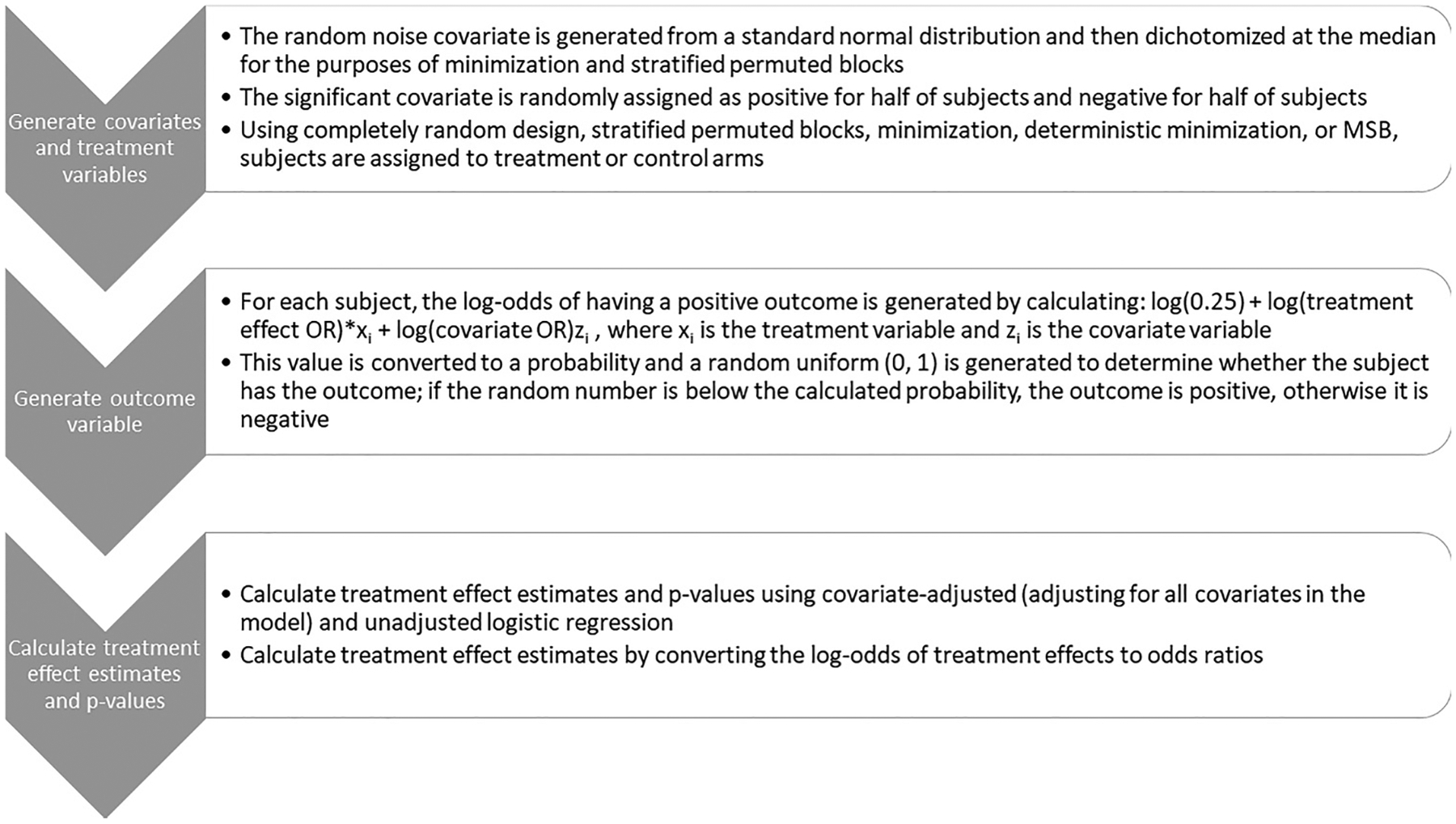
Flow chart of simulation study procedure. x represents the treatment variable, and z represents the potential confounding covariate.

Although the estimates of covariate and treatment effects asymptotically converge to the true covariate and treatment effects when maximum likelihood estimation is used, it should be noted that estimates of covariate and treatment effects are subject to bias in modeling, particularly with small sample sizes. This consideration is especially important when covariates that are related to the outcome are involved in the simulations, whether or not the covariates are adjusted for in the final analysis.^9,13,70,71 To compensate for this bias, results from simulations involving stratified permuted blocks, minimization, deterministic minimization, and MSB will be compared with the results of the complete random study design, in addition to the true treatment effects. Thus, the term relative bias will be used to describe the raw difference in the estimation of treatment effect under a particular randomization method and the estimation of treatment effect under the complete randomized method. Relative bias, along with 95% confidence intervals, was generated using the difference in the treatment effect estimates from each trial simulation for each randomization method and the completely randomized design. Underlying normal distribution of treatment effect estimates was assumed. Similarly, the term relative power will be used to describe the difference in the estimation of power to detect a treatment effect under a particular randomization method and the estimation of power to detect a treatment effect under the complete randomized method. Relative power, along with 95% confidence intervals, was generated using the difference in the proportion of trials which rejected the null hypothesis from each trial simulation for each randomization method and the completely randomized design. The analysis was done using a normal approximation of the binomial distribution.

Permutation tests were also included for comparison. Permutation tests are nonparametric and therefore are useful also in examining the sensitivity of the various methods to distributional assumptions.⁷² Because of the computational complexity of calculating effect sizes for every possible combination of treatment assignments for 50, 100 or 500 subjects, the method of Phipson and Smyth⁷³ was used. To calculate p-value using permutation tests, 1000 permutations of the treatment variables were randomly generated using the relevant randomization method and the p-value was calculated as the sum of the number of odds ratios from permutations that were above the observed odds ratio and below the inverse of the odds ratio, divided by 1000.

Prevalence of the outcome for different simulation scenarios depended on the fixed covariate odds ratio and the effect size. Therefore, the prevalence varied between simulation scenarios. Preliminary analyses found that fixing the prevalence in addition to odds ratio and effect size led to scarcity of the outcome for some combinations of treatment and covariates, causing some simulations to fail to converge. However, to study the impact of the varying prevalence, a scenario where the odds ratio is fixed (at 2), with a random noise covariate at a sample size of 500, prevalence was fixed at 20%, 35%, and 50% and simulations were performed.

3. Results

In Tables 1, 2, 3, and 4, power and bias in the estimation of treatment effect are presented for the various covariate balancing approaches (namely, complete randomization, permuted blocks, minimization, deterministic minimization, and MSB). In each of these tables, covariate imbalance is controlled on a random noise covariate, and may be adjusted for covariates. It should be noted that in Tables 3 and 4, the power consistently exceeds 80% across all methods. This is because the study was powered to detect treatment effects under the assumption that there was no confounding variable, as is commonly done in clinical trials. Thus, the potential confounding covariate influences the power to detect the treatment effect. Tables 5, 6, 7, and 8 show, for the same scenarios, relative bias and relative power for each randomization method compared with complete randomization. Tables 1 and 5 show results with only a random noise covariate and an unadjusted endpoint (Model 1). Tables 2 and 6 show results with only a random noise covariate and a covariate-adjusted endpoint (Model 2). Tables 3 and 7 show results with a random noise covariate and a covariate which is related to the outcome variable, and an unadjusted endpoint (Model 3). Tables 4 and 8 show results with a random noise covariate and a covariate which is related to the outcome variable, and a covariate-adjusted endpoint (Model 4).

Table 1.

Comparing power and bias in treatment effect estimation across methods balancing on a random noise covariate in unadjusted simulations (model 1).

	n = 50		n = 100		n = 500
	Treatment OR: 5.64		Treatment OR: 3.45		Treatment OR: 1.79
	Prevalence: 0.393 (0.264, 0.528)		Prevalence: 0.332 (0.248, 0.431)		Prevalence: 0.255 (0.218, 0.295)
Method	Bias	Power	Bias	Power	Bias	Power
CR	0.215 (0.202, 0.228)	0.805 (0.797, 0.813)	0.039 (0.030, 0.048)	0.804 (0.796, 0.812)	0.003 (−0.001, 0.007)	0.802 (0.794, 0.810)
SPB	0.187 (0.159, 0.214)	0.821 (0.813, 0.829)	0.039 (0.030, 0.048)	0.806 (0.798, 0.814)	0.005 (0.001, 0.009)	0.798 (0.790, 0.806)
Min.	0.215 (0.185, 0.246)	0.805 (0.797, 0.813)	0.039 (0.030, 0.048)	0.804 (0.796, 0.812)	0.003 (−0.001, 0.007)	0.802 (0.794, 0.810)
D. Min.	0.215 (0.185, 0.246)	0.805 (0.797, 0.813)	0.039 (0.030, 0.048)	0.804 (0.796, 0.812)	0.003 (−0.001, 0.007)	0.802 (0.794, 0.809)
MSB	0.215 (0.185, 0.246)	0.805 (0.797, 0.813)	0.039 (0.030, 0.048)	0.804 (0.796, 0.812)	0.003 (−0.001, 0.007)	0.802 (0.794, 0.810)

Results are presented as estimate (95% CI). The block size used was 6, the biased coin probability used is 0.65, and the p-value threshold is 0.3. Note that treatment effects were calculated to obtain 80% power to detect a treatment effect in the absence of covariates.

CR: completely randomized design; D. Min: deterministic minimization; Min: minimization with a biased coin; MSB: minimal sufficient balance; SPB: stratified permuted blocks.

Table 2.

Comparing power and bias in treatment effect estimation across methods balancing on a random noise covariate in covariate-adjusted simulations (model 2).

	n = 50		n = 100		n = 500
	Treatment OR: 5.64		Treatment OR: 3.45		Treatment OR: 1.79
	Prevalence: 0.393 (0.264, 0.528)		Prevalence: 0.332 (0.248, 0.431)		Prevalence: 0.255 (0.218, 0.295)
Method	Bias	Power	Bias	Power	Bias	Power
CR	0.266 (0.235, 0.297)	0.800 (0.792, 0.808)	0.054 (0.045, 0.064)	0.804 (0.796, 0.812)	0.004 (−0.000, 0.008)	0.800 (0.792, 0.808)
SPB	0.234 (0.206, 0.261)	0.819 (0.811, 0.827)	0.054 (0.044, 0.063)	0.807 (0.799, 0.815)	0.006 (0.002, 0.010)	0.798 (0.790, 0.806)
Min.	0.206 (0.180, 0.232)	0.810 (0.802, 0.818)	0.050 (0.040, 0.060)	0.812 (0.804, 0.820)	0.005 (0.001, 0.009)	0.794 (0.786, 0.802)
D. Min.	0.187 (0.163, 0.211)	0.813 (0.163, 0.211)	0.047 (0.038, 0.057)	0.808 (0.800, 0.816)	0.004 (−0.000, 0.008)	0.798 (0.790, 0.806)
MSB	0.228 (0.200, 0.255)	0.805 (0.797, 0.813)	0.050 (0.041, 0.060)	0.802 (0.794, 0.810)	0.005 (0.000, 0.009)	0.797 (0.789, 0.805)

Results are presented as estimate (95% CI). CR represents completely randomized design. The block size used was 6, the biased coin probability used is 0.65, and the p-value threshold is 0.3. Note that treatment effects were calculated to obtain 80% power to detect a treatment effect in the absence of covariates. CR: completely randomized design; D. Min: deterministic minimization; Min: minimization with a biased coin; MSB: minimal sufficient balance; SPB: stratified permuted blocks.

Table 3.

Comparing power and bias in treatment effect estimation across methods with random noise covariate and a covariate with an effect on the outcome (OR = 1.5, 2, 5) in unadjusted simulations (model 3).

		n = 50		n = 100		n = 500
		Treatment OR: 5.64		Treatment OR: 3.45		Treatment OR: 1.79
Covariate OR	Method	Bias	Power	Bias	Power	Bias	Power
1.5	Prevalence: 0.434 (0.300, 0.568)		Prevalence: 0.375 (0.285, 0.472)		Prevalence: 0.296 (0.256, 0.338)
	CR	0.133 (0.110, 0.155)	0.814 (0.807, 0.822)	0.021 (0.012, 0.030)	0.824 (0.817, 0.832)	−0.002 (−0.006, 0.002)	0.831 (0.824, 0.839)
	SPB	0.107 (0.087, 0.126)	0.818 (0.810, 0.825)	0.023 (0.014, 0.032)	0.825 (0.817, 0.832)	−0.004 (−0.008, −0.000)	0.826 (0.819, 0.833)
	Min.	0.133 (0.110, 0.155)	0.814 (0.807, 0.822)	0.021 (0.012, 0.030)	0.825 (0.817, 0.832)	−0.002 (−0.006, 0.002)	0.831 (0.824, 0.839)
	D. Min.	0.133 (0.110, 0.155)	0.814 (0.807, 0.822)	0.021 (0.012, 0.030)	0.824 (0.817, 0.832)	−0.002 (−0.006, 0.002)	0.831 (0.824, 0.839)
	MSB	0.133 (0.110, 0.155)	0.814 (0.807, 0.822)	0.021 (0.012, 0.030)	0.825 (0.817, 0.832)	−0.002 (−0.006, 0.002)	0.831 (0.824, 0.839)
2	Prevalence: 0.464 (0.337, 0.607)		Prevalence: 0.407 (0.313, 0.503)		Prevalence: 0.329 (0.289, 0.371)
	CR	0.074 (0.056, 0.093)	0.813 (0.805, 0.821)	−0.004 (−0.013, 0.005)	0.823 (0.816, 0.830)	−0.013 (−0.017, 0.010)	0.839 (0.832, 0.846)
	SPB	0.049 (0.033, 0.064)	0.810 (0.802, 0.818)	−0.004 (−0.012, 0.005)	0.826 (0.819, 0.833)	−0.014 (−0.017, −0.010)	0.841 (0.834, 0.848)
	Min.	0.074 (0.056, 0.093)	0.813 (0.805, 0.821)	−0.004 (−0.013, 0.005)	0.823 (0.816, 0.830)	−0.013 (−0.017, −0.010)	0.839 (0.832, 0.846)
	D. Min.	0.074 (0.056, 0.093)	0.813 (0.805, 0.821)	−0.004 (−0.013, 0.005)	0.823 (0.816, 0.830)	−0.013 (−0.017, −0.010)	0.839 (0.832, 0.846)
	MSB	0.074 (0.056, 0.093)	0.813 (0.805, 0.821)	−0.004 (−0.013, 0.005)	0.823 (0.816, 0.830)	−0.013 (−0.017, 0.010)	0.839 (0.832, 0.846)
5	Prevalence: 0.554 (0.413, 0.682)		Prevalence: 0.508 (0.408, 0.602)		Prevalence: 0.439 (0.396, 0.483)
	CR	−0.128 (−0.143, −0.112)	0.721 (0.712, 0.730)	−0.148 (−0.156, −0.140)	0.749 (0.741, 0.757)	−0.082 (−0.086, −0.078)	0.781 (0.773, 0.789)
	SPB	−0.160 (−0.173, −0.146)	0.723 (0.714, 0.732)	−0.151 (−0.159, −0.143)	0.758 (0.750, 0.766)	−0.082 (−0.086, −0.078)	0.786 (0.778, 0.794)
	Min.	−0.128 (−0.143, −0.112)	0.721 (0.712, 0.730)	−0.148 (−0.156, −0.140)	0.749 (0.741, 0.757)	−0.082 (−0.086, −0.078)	0.781 (0.773, 0.789)
	D. Min.	−0.128 (−0.143, −0.112)	0.721 (0.712, 0.730)	−0.148 (−0.156, −0.140)	0.749 (0.741, 0.758)	−0.082 (−0.086, −0.078)	0.781 (0.773, 0.790)
	MSB	−0.128 (−0.143, −0.112)	0.721 (0.712, 0.730)	−0.148 (−0.156, −0.140)	0.749 (0.741, 0.757)	−0.082 (−0.086, −0.078)	0.781 (0.773, 0.789)

Results are presented as estimate (95% CI). The block size used was 6, the biased coin probability used is 0.65, and the p-value threshold is 0.3. Note that treatment effects were calculated to obtain 80% power to detect a treatment effect in the absence of covariates. CR: completely randomized design; D. Min: deterministic minimization; Min: minimization with a biased coin; MSB: minimal sufficient balance; SPB: stratified permuted blocks.

Table 4.

Comparing power and bias in treatment effect estimation across methods with random noise covariate and a covariate with an effect on the outcome (OR = 1.5, 2, 5) in covariate-adjusted simulations (model 4).

		n = 50		n = 100		n = 500
		Treatment OR: 5.64		Treatment OR: 3.45		Treatment OR: 1.79
Covariate OR	Method	Bias	Power	Bias	Power	Bias	Power
1.5	Prevalence: 0.434 (0.300, 0.568)		Prevalence: 0.375 (0.285, 0.472)		Prevalence: 0.296 (0.256, 0.338)
	CR	0.277 (0.250, 0.304)	0.816 (0.809, 0.824)	0.063 (0.054, 0.072)	0.825 (0.818, 0.833)	0.005 (0.001, 0.009)	0.833 (0.826, 0.841)
	SPB	0.231 (0.208, 0.253)	0.829 (0.822, 0.837)	0.065 (0.055, 0.074)	0.827 (0.819, 0.834)	0.003 (−0.001, 0.007)	0.831 (0.824, 0.838)
	Min.	0.204 (0.185, 0.222)	0.824 (0.817, 0.832)	0.062 (0.053, 0.071)	0.828 (0.820, 0.835)	0.005 (0.001, 0.009)	0.837 (0.830, 0.844)
	D. Min.	0.215 (0.195, 0.234)	0.832 (0.825, 0.840)	0.056 (0.047, 0.065)	0.834 (0.827, 0.842)	0.007 (0.003, 0.011)	0.835 (0.827, 0.842)
	MSB	0.240 (0.217, 0.263)	0.814 (0.807, 0.822)	0.061 (0.052, 0.070)	0.823 (0.816, 0.830)	0.004 (0.000, 0.008)	0.828 (0.820, 0.835)
2	Prevalence: 0.464 (0.337, 0.607)		Prevalence: 0.407 (0.313, 0.503)		Prevalence: 0.329 (0.289, 0.371)
	CR	0.269 (0.244, 0.295)	0.818 (0.810, 0.826)	0.062 (0.052, 0.071)	0.829 (0.822, 0.836)	0.004 (0.000, 0.008)	0.848 (0.841, 0.855)
	SPB	0.232 (0.210, 0.254)	0.828 (0.821, 0.835)	0.063 (0.053, 0.072)	0.837 (0.830, 0.844)	0.003 (−0.001, 0.007)	0.847 (0.840, 0.854)
	Min.	0.212 (0.192, 0.232)	0.825 (0.818, 0.832)	0.064 (0.055, 0.073)	0.836 (0.829, 0.843)	0.005 (0.001, 0.009)	0.850 (0.843, 0.857)
	D. Min.	0.214 (0.195, 0.234)	0.830 (0.822, 0.837)	0.056 (0.047, 0.065)	0.839 (0.831, 0.846)	0.007 (0.003, 0.011)	0.849 (0.842, 0.856)
	MSB	0.239 (0.216, 0.262)	0.814 (0.806, 0.822)	0.058 (0.049, 0.067)	0.831 (0.824, 0.838)	0.005 (0.001, 0.009)	0.844 (0.837, 0.851)
5	Prevalence: 0.554 (0.413, 0.682)		Prevalence: 0.508 (0.408, 0.602)		Prevalence: 0.439 (0.396, 0.483)
	CR	0.494 (0.447, 0.542)	0.749 (0.741, 0.747)	0.069 (0.059, 0.079)	0.796 (0.788, 0.804	0.004 (0.000, 0.008)	0.839 (0.832, 0.846)
	SPB	0.414 (.372, 0.456)	0.763 (0.755, 0.771)	0.072 (0.062, 0.083)	0.800 (0.792, 0.808)	0.003 (−0.001, 0.007)	0.839 (0.832, 0.846)
	Min.	0.375 (0.336, 0.414)	0.761 (0.753, 0.769)	0.073 (0.063, 0.082)	0.805 (0.797, 0.813)	0.006 (0.002, 0.010)	0.842 (0.835, 0.849)
	D. Min.	0.398 (0.357, 0.438)	0.768 (0.760, 0.776)	0.061 (0.052, 0.071)	0.801 (0.793, 0.809)	0.008 (0.004, 0.012)	0.842 (0.835, 0.850)
	MSB	0.447 (0.403, 0.491)	0.751 (0.743, 0.759)	0.070 (0.059, 0.080)	0.795 (0.787, 0.803)	0.006 (0.002, 0.009)	0.843 (0.836, 0.850)

Results are presented as estimate (95% CI). The block size used was 6, the biased coin probability used is 0.65, and the p-value threshold is 0.3. Note that treatment effects were calculated to obtain 80% power to detect a treatment effect in the absence of covariates. CR: completely randomized design; D. Min: deterministic minimization; Min: minimization with a biased coin; MSB: minimal sufficient balance; SPB: stratified permuted blocks.

Table 5.

Comparing relative power and relative bias across methods balancing on a random noise covariate in unadjusted simulations (model 1).

	n = 50		n = 100		n = 500
	Treatment OR: 5.64		Treatment OR: 3.45		Treatment OR: 1.79
	Prevalence: 0.393 (0.264, 0.528)		Prevalence: 0.332 (0.248, 0.431)		Prevalence: 0.255 (0.218, 0.295)
Method	Relative bias	Relative power	Relative bias	Relative power	Relative bias	Relative power
SPB	−0.029 (−0.047, −0.011)	0.016 (0.005, 0.027)	0.000 (−0.013, 0.013)	0.002 (−0.009, 0.013)	0.002 (−0.004, 0.008)	−0.004 (−0.015, 0.007)
Min.	0.000 (−0.018, 0.018)	0.000 (−0.011, 0.011)	0.000 (−0.013, 0.013)	0.000 (−0.011, 0.011)	0.000 (−0.006, 0.006)	0.000 (−0.011, 0.011)
D. Min.	0.000 (−0.018, 0.018)	0.000 (−0.011, 0.011)	0.000 (−0.013, 0.013)	0.000 (−0.011, 0.011)	0.000 (−0.006, 0.006)	0.000 (−0.011, 0.011)
MSB	0.000 (−0.018, 0.018)	0.000 (−0.011, 0.011)	0.000 (−0.013, 0.013)	0.000 (−0.011, 0.011)	0.000 (−0.006, 0.006)	0.000 (−0.011, 0.011)

Results are presented as estimate (95% CI). The block size used was 6, the biased coin probability used is 0.65, and the p-value threshold is 0.3. Note that treatment effects were calculated to obtain 80% power to detect a treatment effect in the absence of covariates. CR: completely randomized design; D. Min: deterministic minimization; Min: minimization with a biased coin; MSB: minimal sufficient balance; SPB: stratified permuted blocks.

Table 6.

Comparing relative power and relative bias across methods balancing on a random noise covariate in covariate-adjusted simulations (model 2).

	n = 50		n = 100		n = 500
	Treatment OR: 5.64		Treatment OR: 3.45		Treatment OR: 1.79
	Prevalence: 0.393 (0.264, 0.528)		Prevalence: 0.332 (0.248, 0.431)		Prevalence: 0.255 (0.218, 0.295)
Method	Relative bias	Relative power	Relative bias	Relative power	Relative bias	Relative power
SPB	−0.033 (−0.052, −0.014)	0.019 (0.008, 0.030)	0.000 (−0.013, 0.013)	0.003 (−0.008, 0.014)	0.002 (−0.004, 0.008)	−0.002 (−0.013, 0.009)
Min.	−0.060 (−0.079, −0.041)	0.010 (−0.001, 0.021)	−0.004 (−0.017, 0.009)	0.008 (−0.003, 0.019)	0.001 (−0.005, 0.007)	−0.006 (−0.017, 0.005)
D. Min.	−0.079 (−0.098, −0.060)	0.013 (0.002, 0.024)	−0.007 (−0.020, 0.006)	0.004 (−0.007, 0.015)	0.000 (−0.006, 0.006)	−0.002 (−0.013, 0.009)
MSB	−0.039 (−0.058, −0.020)	0.005 (−0.006, 0.016)	−0.004 (−0.017, 0.009)	−0.002 (−0.013, 0.009)	0.001 (−0.005, 0.007)	−0.003 (−0.014, 0.008)

Results are presented as estimate (95% CI). The block size used was 6, the biased coin probability used is 0.65, and the p-value threshold is 0.3. Note that treatment effects were calculated to obtain 80% power to detect a treatment effect in the absence of covariates. CR: completely randomized design; D. Min: deterministic minimization; Min: minimization with a biased coin; MSB: minimal sufficient balance; SPB: stratified permuted blocks.

Table 7.

Comparing relative power and relative bias across methods with random noise covariate and a covariate with an effect on the outcome (OR = 1.5, 2, 5) in unadjusted simulations (model 3).

		n = 50		n = 100		n = 500
		Treatment OR: 5.64		Treatment OR: 3.45		Treatment OR: 1.79
Covariate OR	Method	Relative bias	Relative power	Relative bias	Relative power	Relative bias	Relative power
1.5	Prevalence: 0.434 (0.300, 0.568)		Prevalence: 0.375 (0.285, 0.472)		Prevalence: 0.296 (0.256, 0.338)
	SPB	−0.026 (−0.044, −0.008)	0.004 (−0.007, 0.015)	0.002 (−0.010, 0.014)	0.001 (−0.010, 0.012)	−0.004 (−0.010, 0.002)	−0.005 (−0.015, 0.005)
	Min.	0.000 (−0.018, 0.018)	0.000 (−0.011, 0.011)	0.000 (−0.012, 0.012)	0.000 (−0.011, 0.011)	−0.002 (−0.008, 0.004)	0.000 (−0.010, 0.010)
	D. Min.	0.000 (−0.018, 0.018)	0.000 (−0.011, 0.011)	0.000 (−0.012, 0.012)	0.000 (−0.011, 0.011)	−0.002 (−0.008, 0.004)	0.000 (−0.010, 0.010)
	MSB	0.000 (−0.018, 0.018)	0.000 (−0.011, 0.011)	0.000 (−0.012, 0.012)	0.000 (−0.011, 0.011)	−0.002 (−0.008, 0.004)	0.000 (−0.010, 0.010)
2	Prevalence: 0.464 (0.337, 0.607)		Prevalence: 0.407 (0.313, 0.503)		Prevalence: 0.329 (0.289, 0.371)
	SPB	−0.026 (−0.044, −0.008)	−0.003 (−0.014, 0.008)	0.000 (−0.012, 0.012)	0.003 (−0.008, 0.014)	−0.001 (−0.006, 0.004)	0.002 (−0.008, 0.012)
	Min.	0.000 (−0.018, 0.018)	0.000 (−0.011, 0.011)	0.000 (−0.012, 0.012)	0.000 (−0.011, 0.011)	0.000 (−0.005, 0.005)	0.000 (−0.010, 0.010)
	D. Min.	0.000 (−0.018, 0.018)	0.000 (−0.011, 0.011)	0.000 (−0.012, 0.012)	0.000 (−0.011, 0.011)	0.000 (−0.005, 0.005)	0.000 (−0.010, 0.010)
	MSB	0.000 (−0.018, 0.018)	0.000 (−0.011, 0.011)	0.000 (−0.012, 0.012)	0.000 (−0.011, 0.011)	0.000 (−0.005, 0.005)	0.000 (−0.010, 0.010)
5	Prevalence: 0.554 (0.413, 0.682)		Prevalence: 0.508 (0.408, 0.602)		Prevalence: 0.439 (0.396, 0.483)
	SPB	−0.032 (−0.049, −0.014)	0.002 (−0.010, 0.014)	−0.003 (−0.015, 0.009)	0.009 (−0.003, 0.021)	0.000 (−0.005, 0.005)	0.005 (−0.006, 0.016)
	Min.	0.000 (−0.017, 0.017)	0.000 (−0.012, 0.012)	0.000 (−0.012, 0.012)	0.000 (−0.012, 0.012)	0.000 (−0.005, 0.005)	0.000 (−0.011, 0.011)
	D. Min.	0.000 (−0.017, 0.017)	0.000 (−0.012, 0.012)	0.000 (−0.012, 0.012)	0.000 (−0.012, 0.012)	0.000 (−0.005, 0.005)	0.000 (−0.011, 0.011)
	MSB	0.000 (−0.017, 0.017)	0.000 (−0.012, 0.012)	0.000 (−0.012, 0.012)	0.000 (−0.012, 0.012)	0.000 (−0.005, 0.005)	0.000 (−0.011, 0.011)

Results are presented as estimate (95% CI). The block size used was 6, the biased coin probability used is 0.65, and the p-value threshold is 0.3. Note that treatment effects were calculated to obtain 80% power to detect a treatment effect in the absence of covariates. CR: completely randomized design; D. Min: deterministic minimization; Min: minimization with a biased coin; MSB: minimal sufficient balance; SPB: stratified permuted blocks.

Table 8.

Comparing relative power and relative bias across methods with random noise covariate and a covariate with an effect on the outcome (OR = 1.5, 2, 5) in covariate-adjusted simulations (model 4).

		n = 50		n = 100		n = 500
		Treatment OR: 5.64		Treatment OR: 3.45		Treatment OR: 1.79
Covariate OR	Method	Relative bias	Relative power	Relative bias	Relative power	Relative bias	Relative power
1.5	Prevalence: 0.434 (0.300, 0.568)		Prevalence: 0.375 (0.285, 0.472)		Prevalence: 0.296 (0.256, 0.338)
	SPB	−0.046 (−0.065, −0.027)	0.013 (0.002, 024)	0.002 (−0.011, 0.015)	0.002 (−0.009, 0.013)	−0.002 (−0.008, 0.004)	−0.002 (−0.012, 0.008)
	Min.	−0.073 (−0.092, −0.048)	−0.006 (−0.017, 0.005)	−0.001 (−0.012, 0.014)	0.003 (−0.010, 0.016)	0.000 (−0.006, 0.006)	0.004 (−0.006, 0.014)
	D. Min.	−0.062 (−0.074, −0.050)	0.016 (0.005, 0.027)	−0.007 (−0.020, 0.006)	0.009 (−0.004, 0.022)	0.002 (−0.004, 0.008)	0.002 (−0.008, 0.012)
	MSB	−0.037 (−0.056, −0.018)	−0.001 (−0.012, 0.010)	−0.002 (−0.015, 0.011)	−0.002 (−0.013, 0.009)	−0.001 (−0.007, 0.005)	−0.005 (−0.015, 0.005)
2	Prevalence: 0.464 (0.337, 0.607)		Prevalence: 0.407 (0.313, 0.503)		Prevalence: 0.329 (0.289, 0.371)
	SPB	−0.038 (−0.057, −0.019)	0.010 (−0.001, 0.021)	0.001 (−0.011, 0.013)	0.008 (−0.002, 0.018)	−0.001 (−0.006, 0.004)	−0.001 (−0.011, 0.009)
	Min.	−0.058 (−0.077, −0.039)	0.007 (−0.004, 0.018)	0.002 (−0.010, 0.014)	0.007 (−0.003, 0.017)	0.001 (−0.004, 0.006)	0.002 (−0.008, 0.012)
	D. Min.	−0.055 (−0.074, −0.036)	0.012 (0.001, 0.023)	−0.006 (−0.018, 0.006)	0.010 (−0.000, 0.020)	0.003 (−0.002, 0.008)	0.001 (−0.009, 0.011)
	MSB	−0.031 (−0.050, −0.012)	−0.004 (−0.015, 0.007)	−0.004 (−0.016, 0.008)	0.002 (−0.008, 0.012)	0.001 (−0.004, 0.006)	−0.004 (−0.014, 0.006)
5	Prevalence: 0.554 (0.413, 0.682)		Prevalence: 0.508 (0.408, 0.602)		Prevalence: 0.439 (0.396, 0.483)
	SPB	−0.081 (−0.101, −0.061)	0.014 (0.002, 0.026)	0.003 (−0.010, 0.016)	0.004 (−0.007, 0.015)	−0.001 (−0.006, 0.004)	0.000 (−0.010, 0.010)
	Min.	−0.119 (−0.139, −0.099)	0.012 (0.000, 0.024)	0.004 (−0.009, 0.017)	0.009 (−0.002, 0.020)	0.002 (−0.003, 0.007)	0.003 (−0.007, 0.013)
	D. Min.	−0.096 (−0.116, −0.076)	0.019 (0.007, 0.031)	−0.008 (−0.021, 0.005)	0.005 (−0.006, 0.016)	0.004 (−0.001, 0.009)	0.003 (−0.007, 0.013)
	MSB	−0.048 (−0.069, −0.027)	0.002 (−0.010, 0.014)	0.001 (−0.012, 0.014)	−0.001 (—0.012, 0.010)	0.002 (−0.003, 0.007)	0.004 (−0.006, 0.014)

Results are presented as estimate (95% CI). The block size used was 6, the biased coin probability used is 0.65, and the p-value threshold is 0.3. Note that treatment effects were calculated to obtain 80% power to detect a treatment effect in the absence of covariates. CR: completely randomized design; D. Min: deterministic minimization; Min: minimization with a biased coin; MSB: minimal sufficient balance; SPB: stratified permuted blocks.

All simulations involving minimization and MSB where no covariate adjustment was made had no statistically significant differences in bias or power in the estimation of treatment effect compared with complete randomized design (see Tables 5 and 7). In the case of small sample sizes (n = 50) when imbalance was only controlled on the random noise covariate, stratified permuted blocks randomization had a relative bias of −0.029 (95% CI: −0.047 to −0.011) and higher relative power of 0.016 (95% CI: 0.005, 0.027) (see Table 5). Simulations using larger sample sizes (n = 100, 500) did not find statistically significant differences in bias and power compared with complete randomized designs under all randomization methods (see Tables 5 and 7).

Simulations under Model 2 involving minimization with a biased coin and MSB had no statistically significant differences in power to detect treatment effect compared with complete randomized design (see Tables 2 and 6). In the case of small sample sizes (n = 50), stratified permuted blocks randomization had a relative power of 0.019 (95% CI: 0.008, 0.030), and deterministic minimization had a relative power of 0.013 (95% CI: 0.002, 0.024) (see Table 6). In the case of small sample sizes, all four covariate-adaptive randomization methods had covariate estimates that were on average lower than those of the complete randomized design under Model 2. In this case, the relative bias for stratified permuted blocks randomization was −0.033 (95% CI: −0.052 to −0.014), the relative bias for minimization was −0.060 (95% CI: −0.079 to −0.041), the relative bias for deterministic minimization was −0.079 (95% CI: (−0.098, −0.060)), and the relative bias for MSB was −0.039 (95% CI: −0.058 to −0.020) (see Table 6). Simulations using larger sample sizes (n = 100, 500) did not find statistically significant differences in bias and power compared with complete randomized designs under stratified permuted blocks randomization, minimization, deterministic minimization, or MSB.

Under Model 3, where a random noise covariate and a potential confounding covariate are included in the analysis, and the binary endpoint is unadjusted, all simulations involving MSB, minimization, or deterministic minimization had no statistically significant differences in bias and power to detect treatment effect compared with complete randomized design (see Table 7). In the case of small sample sizes (n = 50), stratified permuted blocks randomization compared with complete randomized design had a relative bias of −0.026 (95% CI: −0.044 to −0.008) for an odds ratio of 1.5, −0.026 (95% CI: −0.044 to −0.008) for an odds ratio of 2, and −0.032 (95% CI: −0.049 to −0.014) for an odds ratio of 5. No statistically significant differences in power were found between the complete randomized design and any of the methods under Model 3.

Permutation tests were performed, using a model with a random noise covariate and a covariate whose odds ratio associated with the outcome variable was 2 (n = 50, Model 3). The results showed that there were no significant deviations in the empirical type I error rates between the complete randomized design (p < 0.043; 95% CI: 0.039, 0.047), stratified permuted block randomization (SPB: p < 0.042 95% CI: 0.037, 0.046), minimization (p < 0.043; 95% CI: 0.039, 0.047), deterministic minimization (p < 0.043; 95% CI: 0.039, 0.047), or MSB (p < 0.043; 95% CI: 0.039, 0.047). It should be noted that the empirical type I error rate is below 0.05 across all methods. This is because the study was powered to detect treatment effects under the assumption that there was no variable, other than the treatment effect, that was related to the outcome, as is commonly done in clinical trials.

Simulations involving varied rates of prevalence of the outcome did not reveal any statistically significant differences in results based on prevalence for a sample size of 500 and prevalence of 20%, 35%, and 50%. For the unadjusted analyses, relative bias ranged from −0.001 to 0.001 across all randomization methods, and relative power ranged from 0.000 to 0.002 across all randomization methods. For the covariate-adjusted analyses, relative bias ranged from −0.002 to 0.003 across all randomization methods, and relative power ranged from −0.001 to 0.010 across all randomization methods. None of these deviations were statistically significant.

In Table 4, power and bias in the estimation of treatment effect are presented for the various randomization methods. In the simulations presented in this table, covariate imbalance is being controlled on a random noise covariate as well as a binary covariate, with an odds ratio that changes across sets of simulations between 1.5, 2, and 5 and the outcome is adjusted for covariates (Model 4). For the same scenario, relative bias and relative power, for the four other methods compared with complete randomization, are provided in Table 8. In the case of small sample sizes (n = 50), stratified permuted blocks randomization, minimization, deterministic minimization, and MSB all had average treatment effects which were statistically significantly below that of the complete randomized design for all odds ratios considered. Nonetheless, the most modest deviations were from simulations involving MSB, and the most extreme deviations were from simulations involving minimization with a biased coin. For example, in simulations involving minimization with a random noise covariate and a covariate with an odds ratio of 5 with a covariate-adjusted binary endpoint, the relative bias was −0.081 (95% CI: −0.101 to −0.061) under stratified permuted blocks randomization, −0.119 (95% CI: −0.139 to −0.099) under minimization, −0.096 (95% CI: −0.116 to −0.076) under deterministic minimization, and −0.048 (95% CI: −0.069 to −0.027) under MSB (see Table 8).

Power to detect treatment effect was not statistically significantly different from the complete randomized design in any simulations involving MSB (see Tables 5, 6, 7, and 8). Simulations involving stratified permuted blocks resulted in statistically significant increases in power from complete randomized design when the endpoint was adjusted for and a potential confounding variable was included in the randomization scheme (Model 4). This occurred in simulations involving a random noise covariate and potential confounding covariate in two cases involving small sample sizes (n = 50): when the odds ratio of the covariate was 1.5 (relative power of 0.013, 95% CI: 0.002, 0.024) and when the odds ratio of the covariate was 5 (relative power of 0.014, 95% CI: 0.002, 0.026) (see Table 8). Simulations involving minimization did result in statistically significant deviations increases in power from complete randomized design when the endpoint was adjusted for and a potential confounding variable was included in the randomization scheme in one of three simulation scenarios (Model 4). This deviation occurred where n = 50 and the odds ratio of the covariate was 5 (relative power of 0.012, 95% CI: 0.000, 0.024). Simulations involving deterministic minimization resulted in statistically significant increases in power from complete randomized design when the endpoint was adjusted for and a potential confounding variable was included in the randomization scheme (Model 4). These deviations occurred where n = 50 and the odds ratio of the covariate was 1.5 (relative power of 0.016, 95% CI: 0.005, 0.027), n = 50 and the odds ratio of the covariate was 2 (relative power of 0.012, 95% CI: 0.001, 0.023), and n = 50 and the odds ratio of the covariate was 5 (relative power of 0.019, 95% CI: 0.007, 0.031).

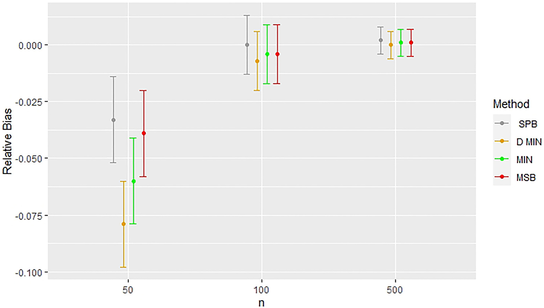
Figures 2 and 3 highlight the consistent issues found in the estimation of treatment effect when stratified permuted blocks were used for randomization with a small sample size (n = 50) in analyses where covariates were not adjusted for (models 1 and 3). In Figures 2 and 3, we see that this deviation in treatment effect estimates exists for n = 50, but no longer exists when n = 100, and n = 500 in unadjusted analyses. All other methods produced almost identical treatment effect estimates, but stratified permuted blocks deviated substantially from all other methods in every modeling situation considered in this study where the outcome was not adjusted for (models 1 and 3). Figure 4 shows that elevated power was found for n = 50 in the model with the random noise covariate and an unadjusted endpoint (Model 1), but this was not the case for the models with a potential confounding variable (Model 3, see Table 7). In the models with the random noise covariate only, the treatment effect estimates improved in the unadjusted analyses for n = 100 and n = 500 (models 1 and 3, sew Tables 5 and 7).

Figure 2.

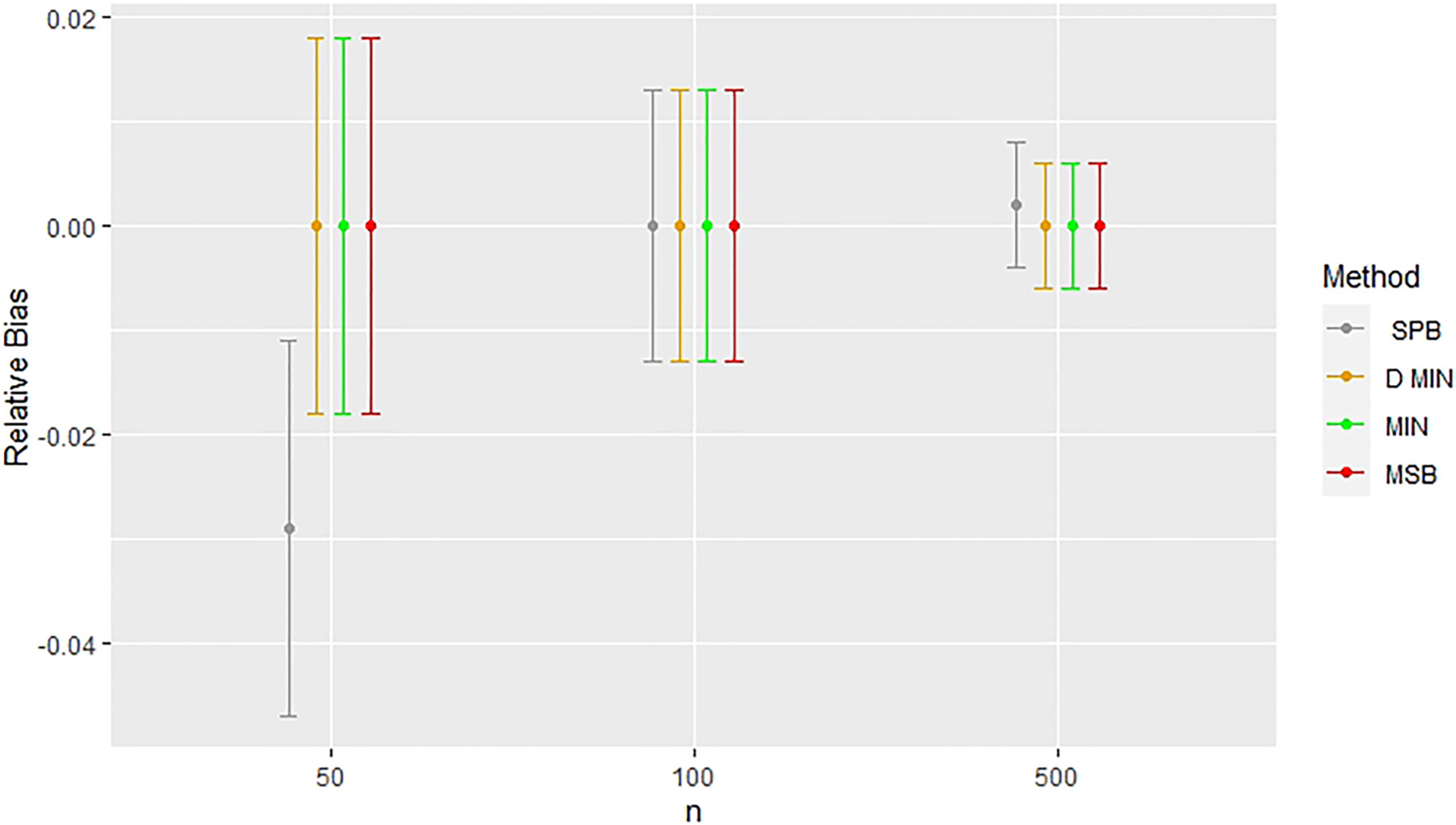
Comparing relative bias across methods with a random noise covariate in unadjusted simulations (Model 1). Error bars represent 95% confidence intervals. Relative bias indicates deviations from results for complete randomization. CR: completely randomized design; D. Min: deterministic minimization; Min: minimization with a biased coin; MSB: minimal sufficient balance; SPB: stratified permuted blocks.

Figure 3.

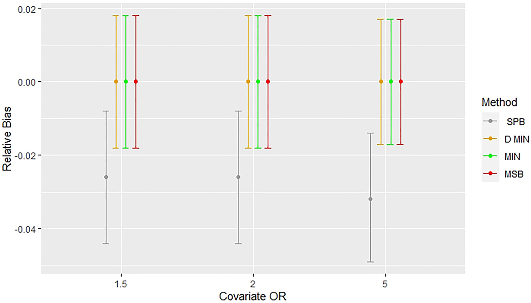
Comparing relative bias across methods with a potential confounding covariate (OR = 1.5,2, 5) and a random noise covariate in unadjusted simulations (Model 3) with n = 50. Error bars represent 95% confidence intervals. Relative bias indicates deviations from results for complete randomization. CR: completely randomized design; D. Min: deterministic minimization; Min: minimization with a biased coin; MSB: minimal sufficient balance; SPB: stratified permuted blocks.

Figure 4.

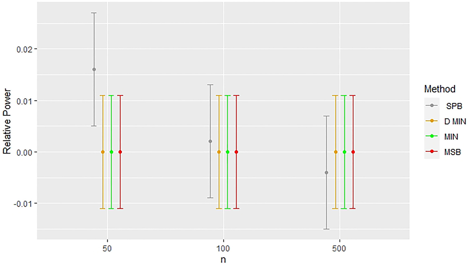
Comparing relative power across methods with a random noise covariate in unadjusted simulations (Model 1). Error bars represent 95% confidence intervals. Relative power indicates deviations from results for complete randomization. CR: completely randomized design; D. Min: deterministic minimization; Min: minimization with a biased coin; MSB: minimal sufficient balance; SPB: stratified permuted blocks.

As discussed previously, bias in covariate-adjusted simulations exist when sample sizes are small (n = 50, models 2 and 4). Treatment effects appear to converge to the estimates found in the complete randomized design as seen in Figure 5. Figures 5 and 6 highlight that the greatest bias, however, is found in covariate-adjusted simulations when minimization with a biased coin is used, followed by deterministic minimization, stratified permuted blocks, and MSB. Figure 7 shows stratified permuted blocks, minimization, and deterministic minimization all have at least one model which shows statistically significant increases in power relative to complete randomized design, whereas MSB does not.

Figure 5.

Comparing relative bias across methods with a random noise covariate in covariate-adjusted simulations (Model 2). Error bars represent 95% confidence intervals. Relative bias indicates deviations from results for complete randomization. CR: completely randomized design; D. Min: deterministic minimization; Min: minimization with a biased coin; MSB: minimal sufficient balance; SPB: stratified permuted blocks.

Figure 6.

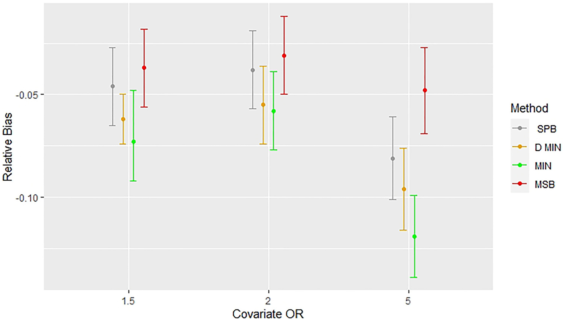
Comparing bias across methods with a potential confounding covariate (OR = 1.5,2, 5) and a random noise covariate in covariate-adjusted simulations (Model 4) with n = 50. Error bars represent 95% confidence intervals. Relative bias indicates deviations from results for complete randomization. CR: completely randomized design; D. Min: deterministic minimization; Min: minimization with a biased coin; MSB: minimal sufficient balance; SPB: stratified permuted blocks.

Figure 7.

Comparing relative power across methods with a potential confounding covariate and a random noise covariate in covariate-adjusted simulations with n = 50 (Model 4), error bars represent 95% confidence intervals. Relative bias indicates deviations from results for complete randomization. CR: completely randomized design; D. Min: deterministic minimization; Min: minimization with a biased coin; MSB: minimal sufficient balance; SPB: stratified permuted blocks.

4. Discussion

Many important conclusions can be made from this simulation study. One major result of this study is that it suggests that minimization (with and without biased coin) and MSB were reliable in unadjusted analyses of treatment effects on a binary endpoint. Results affirm findings of previous research by demonstrating that when stratified permuted blocks are used for randomization, unadjusted analyses can lead to biased treatment effect estimates^42,59 and statistical efficiency may be altered (with respect to power to detect a true treatment effect).^{52,59,60,63–65,68,69} It should be noted that biased treatment effects and altered power were only found in simulations involving stratified permuted blocks with small sample sizes (n = 50). However, there was no evidence – from simulations involving minimization, deterministic minimization, or MSB for all sample sizes and models considered – of biased treatment effect estimates or altered power in unadjusted analyses with a binary endpoint.

A second major finding from this study was that simulations involving MSB demonstrated that, in all cases of models and for all sample sizes, there were no statistically significant differences in the power to detect treatment effects compared with complete randomized design. This was not the case for minimization, deterministic minimization, or stratified permuted blocks and is perhaps a natural consequence of the way MSB is implemented. MSB allows complete randomization to take place for a majority of subjects that are assigned to a treatment arm. A biased coin is only used when a serious imbalance is present, which, as we found in Lauzon et al.¹³ is substantially less often than in minimization. Moreover, when p-values are used to determine serious imbalances, smaller absolute differences are permitted as sample size increases, whereas minimization attempts to control minor imbalances regardless of sample size. Because the MSB method uses fewer biased coin treatment assignments, it more closely resembles complete randomization than minimization.

A third major finding from this study was that in all simulations where covariate adjustment took place with a small sample size (n = 50), treatment effects were biased relative to the findings from the completely randomized design. While the impact of MSB was less than that of stratified permuted blocks and minimization, it is important to consider this bias when deciding to perform covariate-adaptive randomization when the primary analysis is to be adjusted for the covariates included in the randomization method. This consideration is important not only for clinical trials with a small sample size, but for larger trials which have interim analyses which may involve small sample sizes.

A fourth major finding from this study was that there were no significant deviations of power or treatment effect estimation between complete randomized design, stratified permuted blocks, minimization, deterministic minimization and MSB for n = 100 and n = 500. This finding cuts across covariate-adjusted and unadjusted analyses with a binary endpoint. Thus, these methods did not appear to harm the integrity of a trial in any of the modeling situations considered for sample sizes of 100 or greater.

A fifth major finding from this study was that in a modeling situation with two covariates, there were no statistically significant differences between the complete randomized design, stratified permuted block randomization, minimization, deterministic minimization, or MSB with respect to type I error for detecting treatment effect resulting from permutation tests.

This study is meant to complement Lauzon et al.¹³ in comparing and contrasting minimization and MSB in equal allocation sequential clinical trials. In Lauzon et al.,¹³ the stratified permuted blocks method was not considered because of its inability to control imbalance on a large number of covariates. This study considered models with fewer covariates than are typically used for minimization in order to provide a head-to-head comparison with the stratified permuted blocks method, which is widely used in clinical trials. In addition, analyses with a larger number of covariates may be difficult to interpret and results may appear to be too heavily model-dependent. If issues are found with respect to bias and power in treatment effect estimation with a simpler model, it is easier to generalize to a more complex model, as opposed to generalizing across different models of identical complexity. Between both studies, the five aspects which have been considered are: the capacity to control imbalance on several covariates, the proportion of complete randomized treatment assignments, and preservation of the type I error rate, power, and bias in the estimation of treatment effect. Both studies illustrate the preservation of the type I error rate in all covariate-adaptive randomization methods. The stratified permuted blocks method is known (by design) to be unable to control imbalance on a large number of covariates and have a low proportion of complete random treatment designs. Lauzon et al.¹³ showed that for elevated biased coin probabilities (e.g. 0.7 or greater) minimization and MSB were both sufficient for controlling covariate imbalances on five covariates but that the proportion of completely random treatment assignments was far greater for MSB than for minimization in every simulation scenario considered. Allocation randomness remains the most important argument for use of MSB in clinical trials because completely random treatment assignments protects against imbalance of known and unknown covariates and is the basis for inference.¹³

Further research should explore each method in a variety of modeling situations and with different types of outcomes, including continuous outcomes and time-to-event outcomes. Additionally, it should be noted that small differences in power (such as 1–2%) may be statistically significant while not being clinically meaningful in a specific study. However, randomization methods can and should preserve the statistical properties designed for the study, and this study found variations in treatment effect estimation and power to detect treatment effect that can be attributed to the randomization method used. These deviations can permeate in all studies that use these methods and may be expressed even more strongly in other data than what was considered in this study. This study also has limitations inherent to simulation results, and theoretical arguments would provide stronger evidence for the claims made in this study. Additionally, there are many possibilities for models that may use covariate-adaptive randomization, however this study only explores only a few of them. In addition, because deviations across methods occurred only for n = 50, it should be noted that most clinical trials have sample sizes larger than this. Thus, major concerns with respect to bias and power in the estimation of treatment effects should be reserved to small trials and early interim analyses.

Because of increased demand to develop and expand randomization methods that can accommodate unequal allocation,⁷⁴ the randomization methods used in this study should be developed and explored in the context of clinical trials with unequal allocation. MSB is recommended as an alternative to minimization and stratified permuted blocks in equal allocation sequential clinical trials with a binary endpoint when covariate-adaptive randomization is to take place.

References

- 1.Ciolino JD, Martin RH, Zhao W, et al. Continuous covariate imbalance and conditional power for clinical trial interim analyses. Contemp Clin Trials 2014; 38: 9–18. [DOI] [PMC free article] [PubMed] [Google Scholar]
- 2.Simon R. Restricted randomization designs in clinical trials. 1979; 35: 503–512. [PubMed] [Google Scholar]
- 3.Hu F, Hu Y, Ma Z, et al. Adaptive randomization for balancing over covariates. Wiley Interdiscip Rev Comput Stat 2014; 6: 288–303. [Google Scholar]
- 4.Birkett NJ. Adaptive allocation in randomized controlled trials. Control Clin Trials 1985; 6: 146–155. [DOI] [PubMed] [Google Scholar]
- 5.Zhao W and Berger V. Imbalance control in clinical trial subject randomization—from philosophy to strategy. J Clin Epidemiol 2018; 101: 116–118. [DOI] [PubMed] [Google Scholar]
- 6.Sackett D, Rosenberg W, Gray J, et al. Evidence based medicine: what it is and what it isn’t it’s. Br Med J 1996; 312: 71–72. [DOI] [PMC free article] [PubMed] [Google Scholar]
- 7.Bondemark L and Ruf S. Randomized controlled trial: the gold standard or an unobtainable fallacy? Eur J Orthod 2015; 37: 457–461. [DOI] [PubMed] [Google Scholar]
- 8.Senn S. Testing for baseline balance in clinical trials. Stat Med 1997; 13: 1715–1726. [DOI] [PubMed] [Google Scholar]
- 9.Ciolino JD, Martin RH, Zhao W, et al. Covariate imbalance and adjustment for logistic regression analysis of clinical trial data. J Biopharm Stat 2011; 23: 1383–1402. [DOI] [PMC free article] [PubMed] [Google Scholar]
- 10.Yu F. Randomization, stratification, and minimization. In: Principles of clinical trials : bias and precision control. 2019: 1–27. [Google Scholar]
- 11.Kuhn J, Sheldrick RC, Broder-Fingert S, et al. Simulation and minimization: technical advances for factorial experiments designed to optimize clinical interventions. BMC Med Res Methodol 2019; 19: 239. [DOI] [PMC free article] [PubMed] [Google Scholar]
- 12.Zhao W, Hill MD and Palesch Y. Minimal sufficient balance-a new strategy to balance baseline covariates and preserve randomness of treatment allocation. Stat Methods Med Res 2015; 24: 989–1002. [DOI] [PMC free article] [PubMed] [Google Scholar]
- 13.Lauzon SD, Ramakrishnan V, Nietert PJ, et al. Statistical properties of minimal sufficient balance and minimization as methods for controlling baseline covariate imbalance at the design stage of sequential clinical trials. Stat Med 2020. [DOI] [PMC free article] [PubMed] [Google Scholar]
- 14.Simon R Restricted randomization designs in clinical trials. Biometrics 1979; 35(2):503–512. https://www.jstor.org/stable/2530354 [PubMed] [Google Scholar]
- 15.Schulz KF and Grimes DA. Unequal group sizes in randomised trials: guarding against guessing. Lancet 2002; 359: 966–970. doi: 10.1016/S0140-6736(02)08029-7 [DOI] [PubMed] [Google Scholar]
- 16.Kahan BC and Morris TP. Improper analysis of trials randomised using stratified blocks or minimisation. Stat Med 2012; 31: 328–340. [DOI] [PubMed] [Google Scholar]
- 17.Pond GR, Tang PA, Welch SA, et al. Trends in the application of dynamic allocation methods in multi-arm cancer clinical trials. Clin Trials 2010; 7: 227–234. [DOI] [PubMed] [Google Scholar]
- 18.Berger VW, Bejleri K and Agnor R. Comparing MTI randomization procedures to blocked randomization. Stat Med 2016; 35: 685–694. [DOI] [PubMed] [Google Scholar]
- 19.Berger VW, Matthews JR and Grosch EN. On improving research methodology in clinical trials. Stat Methods Med Res 2008; 17: 231–242. [DOI] [PubMed] [Google Scholar]
- 20.McEntegart D. The pursuit of balance using stratified and dynamic randomization techniques: an overview. Drug Inf J 2003; 37: 293–308. [Google Scholar]
- 21.Scott NW, McPherson GC, Ramsay CR, et al. The method of minimization for allocation to clinical trials. a review. Control Clin Trials 2002; 23: 662–674. http://www.ncbi.nlm.nih.gov/pubmed/12505244 [DOI] [PubMed] [Google Scholar]
- 22.Taves DR. Minimization: a new method of assigning patients to treatment and control groups. Clin Pharmacol Ther 1974; 15: 443–453. [DOI] [PubMed] [Google Scholar]
- 23.Pocock SJ and Simon R. Sequential treatment assignment with balancing for prognostic factors in the controlled clinical trial. Biometrics 1975; 31: 103–115. http://www.jstor.org/stable/2529712 [PubMed] [Google Scholar]
- 24.Xu Z, Proschan M and Lee S. Validity and power considerations on hypothesis testing under minimization. Stat Med 2016; 35: 2315–2327. [DOI] [PubMed] [Google Scholar]
- 25.Hannigan JJ, Korety M, McGuigan E, et al. Adaptive randomization biased coin design: experience in a cooperative group clinical trial. Control Clin Trials 1980; 1. [Google Scholar]
- 26.Klotz J. Maximum entropy constrained balance randomization for clinical trials. Int Biometric Soc 1978; 34: 283–287. [PubMed] [Google Scholar]
- 27.Nordle O and Brantmark B. A self-adjusting randomization plan for allocation of patients into two treatment groups. Clin Pharmacol Ther 1977; 22: 825–830. [DOI] [PubMed] [Google Scholar]
- 28.Berger VW. Minimization : not all it ‘ s cracked up to be. Clin Trials 2011; 8. [DOI] [PubMed] [Google Scholar]
- 29.Saghaei M. An Overview of Randomization and Minimization Programs for randomized clinical trials. J Med Signals Sens 2011; 1(1): 55–61. [PMC free article] [PubMed] [Google Scholar]
- 30.Berger VW. Minimization, by its nature, precludes allocation concealment, and invites selection bias. Contemp Clin Trials 2010; 31: 06. [DOI] [PMC free article] [PubMed] [Google Scholar]
- 31.Group T national institute of neurological disorders and stroke rt-P stroke study. Tissue plasminogen activator for acute ischemic stroke. N Engl J Med 2005; 333: 1581–1587. [DOI] [PubMed] [Google Scholar]
- 32.Wang D and Bakhai A. Clinical trials: a practical guide to design, analysis, and reporting. London: Remedica, p. 20036. [Google Scholar]
- 33.Girling D, Parmar M, Stenning S, et al. Cinical trials in cancer: principles and practice. Oxford: Oxford University Press, 2003. [Google Scholar]
- 34.Pocock S. Clinical trials: a practical approach. Chichester: Wiley, 1983. [Google Scholar]
- 35.Altman D. Practical statistics for medical research. London: Chapman and Hall, 1991. [Google Scholar]
- 36.Altman DG and Bland JM. Treatment allocation by minimisation. Br Med J 2005; 330: 43. [DOI] [PMC free article] [PubMed] [Google Scholar]
- 37.Meinert C. Clinical trials: design, conduct, and analysis. Oxford: Oxford University Press, 1986. [Google Scholar]
- 38.Schulz KF and Grimes DA. Generation of allocation sequences in randomised trials: chance, not choice. Lancet 2002; 359: 515–519. [DOI] [PubMed] [Google Scholar]
- 39.Harrington DP. The randomized clinical trial. J Am Stat Assoc 2000; 95: 312–315. [Google Scholar]
- 40.Friedman LM, Furberg CD, DeMets DL, et al. Fundamentals of clinical trials. 2015.
- 41.International Conference on Harmonisation (ICH). ICH harmonised tripartite guideline E9: statistical principles for clinical trials. Stat Med 1999; 18: 1903–1942. http://www.ncbi.nlm.nih.gov/pubmed/10440877 [PubMed] [Google Scholar]
- 42.Raab GM, Day S and Sales J. How to select covariates to include in the analysis of a clinical trial. Control Clin Trials 2000; 21: 330–342. [DOI] [PubMed] [Google Scholar]
- 43.Senn S. Statistical issues in drug development. Chichester: Wiley, 2007. [Google Scholar]
- 44.Redmond C and Colton T. Biostatistics in clinical trials. Chichester: Wiley, 2001. [Google Scholar]
- 45.Piantadosi S Clinical trials: a methodologic perspective. New Jersey: Wiley, 2005. [Google Scholar]
- 46.Lachin JM, Matts JP and Wei JP. Randomization in clinical trials: conclusions and recommendations. Control Clin Trials 1988; 9: 365–374. [DOI] [PubMed] [Google Scholar]
- 47.Kernan WN, Viscoli CM, Makuch RW, et al. Stratified randomization for clinical trials. J Clin Epidemiol 1999; 52: 19–26. [DOI] [PubMed] [Google Scholar]
- 48.Weir CJ and Lees KR. Comparison of stratification and adaptive methods for treatment allocation in an acute stroke clinical trial. Stat Med 2003; 22: 705–726. [DOI] [PubMed] [Google Scholar]
- 49.Hagino A, Hamada C, Yoshimura I, et al. Statistical comparison of random allocation methods in cancer clinical trials. Control Clin Trials 2004; 25: 572–584. [DOI] [PubMed] [Google Scholar]
- 50.Forsythe AB. Validity and power of tests when groups have been balanced for prognostic factors. Comput Stat Data Anal 1987; 5: 193–200. [Google Scholar]
- 51.Rovers MM, Straatman H and Zielhuis GA. Comparison of balanced and random allocation in clinical trials: a simulation study. Eur J Epidemiol 2000; 16: 1123–1129. [DOI] [PubMed] [Google Scholar]
- 52.Kahan BC, Jairath V, Doré CJ, et al. The risks and rewards of covariate adjustment in randomized trials: an assessment of 12 outcomes from 8 studies. Trials 2014; 15: 1–7. [DOI] [PMC free article] [PubMed] [Google Scholar]
- 53.Lachin JM. Properties of simple randomization in clinical trials. Control Clin Trials 1988; 9: 312–326. [DOI] [PubMed] [Google Scholar]
- 54.Kalish LA and Begg CB. Treatment allocation methods in clinical trials: a review. Stat Med 1985; 4: 129–144. [DOI] [PubMed] [Google Scholar]
- 55.Fisher R The arrangement of field experiments. J Min Agric Gt Br. 1926; 33: 83–94. [Google Scholar]
- 56.Efron B Forcing a sequential experiment to be balanced. Biometrika 1971; 58: 403–417. [Google Scholar]
- 57.Wei LJ and Lachin JM. Properties of the urn randomization in clinical trials. Control Clin Trials 1988; 9: 345–364. [DOI] [PubMed] [Google Scholar]
- 58.Atkinson AC. Optimum biased coin designs for sequential clinical trials with prognostic factors. Biometrika 1982; 69: 61–67. [Google Scholar]
- 59.Ciolino JD, Martin RH, Zhao W, et al. Measuring continuous baseline covariate imbalances in clinical trial data. Stat Methods Med Res 2013; 24: 255–272. [DOI] [PMC free article] [PubMed] [Google Scholar]
- 60.Austin PC, Manca A, Zwarenstein M, et al. A substantial and confusing variation exists in handling of baseline covariates in randomized controlled trials: a review of trials published in leading medical journals. J Clin Epidemiol 2010; 63: 142–153. [DOI] [PubMed] [Google Scholar]
- 61.Ciolino JD, Martin RH, Zhao W, et al. Measuring continuous baseline covariate imbalances in clinical trial data. Stat Methods Med Res 2015; 24: 255–272. [DOI] [PMC free article] [PubMed] [Google Scholar]
- 62.Ciolino J, Zhao W, Martin R, et al. Quantifying the cost in power of ignoring continuous covariate imbalances in clinical trial randomization. Contemp Clin Trials 2011; 32: 250–259. [DOI] [PMC free article] [PubMed] [Google Scholar]
- 63.Deddens JA and Petersen MR Approaches for estimating prevalence ratios. Occup Environ Med 2008; 65: 501–506. [DOI] [PubMed] [Google Scholar]
- 64.Ford I and Norrie J. The role of covariates in estimating treatment effects and risk in long-term clinical trials. Stat Med 2002; 21: 2899–2908. [DOI] [PubMed] [Google Scholar]
- 65.Frey JL. Recombinant tissue plasminogen activator (rtPA) for stroke: the perspective at 8 years. Neurologist 2005; 11: 123–133. [DOI] [PubMed] [Google Scholar]
- 66.Ingall TJ, O’Fallon WM, Asplund K, et al. Findings from the reanalysis of the NINDS tissue plasminogen activator for acute ischemic stroke treatment trial. Stroke 2004; 35: 2418–2424. [DOI] [PubMed] [Google Scholar]
- 67.Kalish LA and Begg CB. The impact of treatment allocation procedures on nominal significance levels and bias. Control Clin Trials 1987; 8: 121–135. [DOI] [PubMed] [Google Scholar]
- 68.Robinson LD and Jewell NP. Some surprising results about covariate adjustment in logistic regression models. Int Stat Inst 2006; 59: 227. [Google Scholar]
- 69.Hauck WW, Anderson S and Marcus SM. Should we adjust for covariates in nonlinear regression analyses of randomized trials? Control Clin Trials 1998; 19: 249–256. [DOI] [PubMed] [Google Scholar]
- 70.Gail MH, Wieand S and Piantadosi S. Biased estimates of treatment effect in randomized experiments with nonlinear regressions and omitted covariates. Biometrika 1984; 71: 431–444. [Google Scholar]
- 71.Hernández AV, Steyerberg EW and Habbema JDF. Covariate adjustment in randomized controlled trials with dichotomous outcomes increases statistical power and reduces sample size requirements. J Clin Epidemiol 2004; 57: 454–460. [DOI] [PubMed] [Google Scholar]
- 72.Hasegawa T and Tango T. Permutation test following covariate-adaptive randomization in randomized controlled trials. J Biopharm Stat 2009; 19: 106–119. [DOI] [PubMed] [Google Scholar]
- 73.Phipson B and Smyth GK. Permutation P-values should never be zero: calculating exact P-values when permutations are randomly drawn. Stat Appl Genet Mol Biol 2010; 9: 1–12. [DOI] [PubMed] [Google Scholar]
- 74.Kuznetsova OM and Tymofyeyev Y. Preserving the allocation ratio at every allocation with biased coin randomization and minimization in studies with unequal allocation. Stat Med 2012; 31: 701–723. [DOI] [PubMed] [Google Scholar]
Associated Data
This section collects any data citations, data availability statements, or supplementary materials included in this article.