Expectation-Based Probabilistic Naive Approach for Forecasting Involving Optimized Parameter Estimation

Abstract

This paper presents a forecasting technique based on the principle of naïve approach imposed in a probabilistic sense, thus allowing to express the prediction as the statistical expectation of known observations with a weight involving an unknown parameter. This parameter is learnt from the given data through minimization of error. The theoretical foundation is laid out, and the resulting algorithm is concisely summarized. Finally, the technique is validated on several test functions (and compared with ARIMA and Holt–Winters), special sequences and real-life covid-19 data. Favorable results are obtained in every case, and important insight about the functioning of the technique is gained.

Introduction

Extrapolative forecasting methods are widely used in production and inventory decisions [1], tourism data forecasting [2], economic and financial risk management [3], wind forecasting [4], analyzing and forecasting traffic dynamics [5], forecasting road accidents [6], demographic and epidemiological projection [7], etc. One finds forecasting-related work employing both conventional techniques and machine learning (ML)-based techniques [8], for instance electricity load forecasting using hybrid model based on IEMD, ARIMA, WNN and FOA [9], short-term electricity price forecasting using an adaptive hybrid model based on VMD, SAPSO, SARIMA and DBN [10], and electricity requirement forecasting for smart grid and buildings using ML models, ensemble-based techniques and ANNs [11]. The most recent application of forecasting techniques carried out by various researchers is on the covid-19 data (see for instance [12–16]).

There is a relation between the future and past; however, the knowledge of this relation is not available which calls for developing innovative methods of prediction. Before proceeding to introduce our technique, let us look at the methods proposed/studied in literature. There are a wide range of frequently used quantitative forecasting tools, but most of the focus is still on moving average, simple linear regression based on covariance, and multiple linear regression.

Dedicated forecasting algorithms like ARIMA, SARIMA, Holt–Winters, etc. majorly use integrated moving average after disaggregating into trend, seasonality and white noise. According to Billah et al. [17], applications of exponential smoothing to forecasting time series usually rely on simple exponential smoothing, trend corrected exponential smoothing and a seasonal variation. Their results indicate that the information criterion approaches provide the best basis for automated method selection, where the Akaike information criteria has a slight edge over its information criteria counterparts. Exponential smoothing-based models like Holt–Winters are widely used for forecasting [18]. The interested readers may refer to the work of Chatfield et al. [19] and Armstrong et al. [20] who provide general guidelines for selecting forecasting methods.

Carbonneau et al. [21] applied a representative set of traditional and ML-based forecasting techniques to the demand data and compared the accuracy of the methods. The average performance of the ML techniques did not outperform the traditional deterministic approaches. Efficient training of ML models with ANN, CNN, LSTM, GRU backbones is now possible for deep representation learning. Siami et al. [22] concluded that the average reduction in error rates obtained by LSTM was between 84% and 87% when compared to ARIMA, indicating the superiority of LSTM to ARIMA; however, it is only suitable where ample amount of data and computation resources are available. Problem of overfitting in ML needs to be tackled by different regularization techniques. However, using a support vector machine (SVM) trained on multiple demand series produced the most accurate forecasts. Myrtveit et al. [23] simulated a machine learning and a regression model, based on which they suggested that more reliable research procedures need to be developed before we can have confidence in the conclusions of comparative studies of software prediction models.

Zhang et al. [24] and Khashei et al. [25] created a hybrid model with ARIMA and ANN to capture the linear and nonlinear modeling simultaneously to obtain better accuracy. Hybrid forecasting system based on a dual decomposition strategy and multi-objective optimization was proposed by Yang et al. [26] for electricity price forecasting. In fact, optimization algorithms are widely used to obtain optimal parameters of the forecasting models. It is important since Das et al. [27] concluded that the accuracy of the PV power forecasting model varies by changing the forecast horizon, even with identical forecast model parameters. Zou et al. [28] tried to combine forecasts of individual models with an appropriate weighting scheme to have a predictor with smaller variability so that the accuracy can be improved relative to the use of a selection criterion. Stekler et al. [29] found that combining forecasts does improve accuracy while working on sports forecasting. Also, a need to adjust weights for new and old information is pronounced as prediction may be independent of previous events. Makridakis et al. [30] showed that the statistical methods are more accurate than ML and require lesser computation. Green et al. [31] after comparing 25 papers with quantitative comparisons claimed that complexity (by using more equations, more complex functional forms and more complex interactions) increases forecast error by $27\%$ on an average.

Transdisciplinary transition to distributional or probabilistic forecast has been observed in the past few years. Gneiting et al. [32] formalized and studied notions of calibration in a prediction space setting. Probabilistic forecasts serve as an essential ingredient for optimal decision making since they can quantify uncertainty. Overall, the need for advancement in the methodology of forecasting is immense; thus, researchers constantly look for opportunities to overcome challenges in the field.

This paper proposes an unconventional forecasting approach where the principle of naïve method and average method is modified and simultaneously employed in a probabilistic sense where a parameter is learnt from available data by minimizing an error function, and consequently make a prediction at the unknown point. The paper is organized as follows: Section 2 develops the technique and formally summarizes the algorithm, and Section 3 applies it on several standard mathematical functions, special sequences and a real-life example (covid-19 dataset).

Problem Formulation and Development of Technique

Suppose an analyst is given n data points denoted by $(x_i,y_i)$ for $1\le i\le n$. The objective is to determine $y_{n+1}$ corresponding to the point $x_{n+1}$ where $x_{n+1}\ge x_n$.

The three most basic approaches in literature are: average method, naïve approach, and drift method. In average method, the non-observed value is estimated as the average of past observed values. Naïve approach generates predictions equal to the last observed value, mathematically, $y_{n+1}=y_n$ where $y_n$ is the last data. Modifying this idea to allow slope gives the drift method which is similar to using first and last observation for linear extrapolation to the future. Often there is such a relation where the future is related to the past, however, the knowledge of this relation (or model) is either not available or not accurate, and has uncertainty which clearly indicate that forecasts should be probabilistic. In order to determine $y_{n+1}$ from ${(y_i)}_{1\le i\le n}$, the technique proposed is an agglomeration of naïve approach and average method but in a probabilistic sense as described below.

Since $x_{n+1}$ is near to $x_n$, so the likelihood of $y_{n+1}$ being almost (or exactly) equal to $y_n$ is higher than any other $y_i$. It is quite intuitive that as $x_{n+1}\to x_n$, so $y_{n+1}\to y_n$ for a continuous function. Thus, the value at point $x_{n+1}$ must be most influenced by the value at point $x_n$. Let $y_{n+1}=Y$ be treated as a random variable and $\mathbb{P}[Y=y_i]$ is the probability that $y_{n+1}$ is equal to $y_i$. This probability falls as a point is chosen far away from $x_{n+1}$. Additionally, it must be maximum only at $x_{n+1}$ which is not actually possible since it is the point at which prediction is to be made, so the value is not known beforehand. Keeping these properties in mind, $\mathbb{P}$ can be chosen to obey the Gaussian distribution curve with peak at $x_{n+1}$ with some parameter $\sigma$. Thus, the predicted value of $y_{n+1}$ can be given as the expectation of past data:

$$\begin{array}{c}\hfill {\widehat{y}}_{n+1}=\sum _{i=1}^n{y}_i\mathbb{P}[Y=y_i],\end{array}$$ 1

where

$$\begin{array}{c}\hfill \mathbb{P}[Y=y_i]=\frac{1}{\sigma \sqrt{2\pi }}exp\left(-,\frac{{\left(x_i,-,x_{n+1}\right)}^2}{2{\sigma }^2}\right).\end{array}$$ 2

Here, the parameter $\sigma$ depends on the available data and can be extracted by minimizing the following error function:

$$\begin{array}{c}\hfill E=\sum _{j=1}^{n-1}({\widehat{y}}_{j+1}-y_{j+1}{)}^2,\end{array}$$ 3

which shall give the optimal ${\sigma }^{\ast }=argminE$ that is substituted in (1) to predict $y_{n+1}$.

With (3), one gets good performance for certain standard functions; however, the technique does not perform satisfactorily for functions like $y=log(x)$. This situation can be improved by employing the operating principle on the error function as well, that is, for evaluation at $x_{n+1}$ consider only nearby points in the error function. But reduction of data points is not a wise decision; instead, all data points must be kept but with higher importance assigned to the nearby points. So, we consider the error function given below:

$$\begin{array}{c}\hfill E=\sum _{j=1}^{n-1}({\widehat{y}}_{j+1}-y_{j+1}{)}^2\times \frac{2j}{n(n-1)}\end{array}$$ 4

to determine ${\sigma }^{\ast }$ and then predict $y_{n+1}$. The final technique is concisely given as Algorithm 1.

Results and Discussion

The proposed method is applied to dataset sampled from certain standard functions, special/popular sequences, and real-life dataset like that of covid-19. In this paper, Nelder–Mead algorithm [33] shall be used to minimize the nonlinear loss function. Bottou et al. [34] explained that optimization algorithms such as stochastic gradient descent (SGD) show better performance for large-scale problems. In particular, second-order stochastic gradient and averaged stochastic gradient are asymptotically efficient after a single pass on the training set. Application of this algorithm minimizes the loss function to get the optimal parameter $\sigma$. The optimizer algorithm may be changed; for instance, one may try [35]. Nelder–Mead requires very few function evaluations at each step as it uses a simplex-based direct search method that performs a sequence of transformations of the working simplex, aimed at decreasing the function values at its vertices. Interested readers may apply other optimization techniques to minimize the error function. The experimentation is carried out on an operating environment having Intel(R) Core (TM) i5-10300H CPU with processor speed 4.5 GHz, 16 GB RAM, 1 TB SSD, 8 GB NVIDIA GeForce GTX 1650 graphics processor under 64-bit Windows 10 operating system. The numerical validation of the algorithm is conducted on python coded using open source libraries such as numpy, pandas and matplotlib.

Testing on Standard Functions

The proposed technique is applied to certain functions having different shapes and rate of growth as listed in Table 1. Each test function is sampled at a step size h in the given range. Prediction is made at every point using the data prior to that point. The obtained actual versus predicted plots are shown in Fig. 1 for the considered test functions.

Table 1.

Performance of the proposed technique for different test functions

Function	Range	Step h	Final ${\sigma }^{\ast }$	RMSE	MAPE
x	[1, 50]	0.25	0.2009	0.4809	3.5873
$x^2$	[1, 50]	0.25	0.2021	9.2894	4.1773
$logx$	[1.5, 50]	0.25	0.1999	0.1386	3.3952
$expx$	[1, 30]	0.25	0.5808	2366.0	0.8154
$sin0.1x$	$[1,20\pi ]$	0.25	0.1984	0.0420	10.9208
$cos0.1x$	$[1,20\pi ]$	0.25	0.2002	0.0911	12.9588

Fig. 1.

Plots of actual versus prediction for certain standard functions

For each test function, Table 1 gives the value of root mean squared error (RMSE) and mean absolute percentage error (MAPE) using the error evaluated between the actual curve and the prediction. The actual and predicted data points for selected test functions listed earlier are visualized in Fig. 1 where we observe that the proposed method successfully learns the trend and predicts very close to the actual data. Our method also performs well on periodic trigonometric function like $sinx$ which have alternating slopes.

An interesting revelation comes from Fig. 2 which depicts the prediction for function $sin(x)$ sampled at 0.25, 1.00 and 2.50, respectively. For data points relatively closer to each other, our technique quickly learns and adapts, and thus performs better than other cases. Those working in the field of signal processing might find resemblance of this phenomenon to the Nyquist-Shannon sampling theorem. The output is a flat line for $h=2.5$, it is distorted/phase-shifted (seems non-differentiable) for $h=1$, but for $h=0.25$, the predicted curve initially overestimates then corrects itself over two wavelengths eventually resulting in an almost accurate approximation of the actual curve.

Fig. 2.

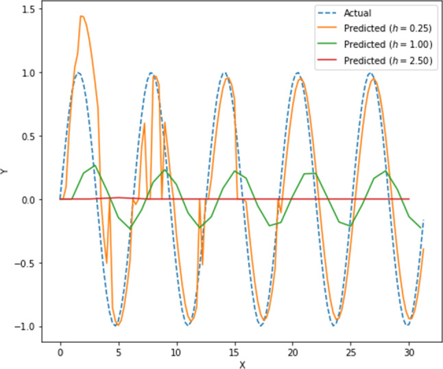
Plot of actual versus predicted for $sin(x)$ with sampling step of 0.25, 1.00 and 2.50

Figure 1 indicates that the prediction is overall accurate except initially. The divergence is a specific property of extrapolation methods and is only circumvented when the functional forms assumed by the method (inadvertently or intentionally due to additional information) accurately represent the nature of the function being extrapolated. In the beginning, the prediction is poor due to insufficient data preceding the point at which prediction is to be made. Eventually, the prediction becomes better and thus better fits the actual curve.

To further strengthen our belief on the proposed technique, it is compared with ARIMA and Holt–Winters. ARIMA refers to autoregressive integrated moving average and is a more complex version of the autoregressive moving average, with the addition of integration. The dependence between an observation and a residual error from a moving average model applied to lagged data is used in this model where the “integrator” aspect makes the time series steady. The Holt–Winters technique is a popular time series forecasting approach that can account for both trend and seasonality. This approach is made up of three different smoothing methods viz. simple exponential smoothing (SES: assumes that the level of the time series remains constant, so cannot be utilized with series that have both trend and seasonality), Holt’s exponential smoothing (HES: it allows trend component in the time series data), and Winter’s exponential smoothing (WES: it is Holt’s exponential smoothing enhancement that finally allows for seasonality to be included).

Figure 3 shows the comparative plot of prediction made in the specific range for linear and exponential functions using ARIMA and Holt–Winters against the point predictions by proposed technique. The process is omitted for other functions since the conclusion remains same or the other methods fail to perform on negative values.

Fig. 3.

Comparative plots of prediction for linear and exponential functions obtained using proposed technique, ARIMA and Holt–Winters; demonstrating better accuracy of the proposed method

Testing on Popular and Special Sequences

The proposed method is also applied to two widely known sequences, namely the Fibonacci and partition sequences. These are described below.

1. Fibonacci Sequence—It is a sequence defined by the recursive relation $F(n)=F(n-2)+F(n-1)$ and is listed as: 1, 1, 2, 3, 5, 8, 13, 21, 34, 55, 89, 144, 233, 377, 610, 987, 1597, 2584, 4181, 6765, 10946, 17711, 28657, 46368, 75025, 121393 and so on, for $n\ge 1$. More information can be found on OEIS [36].

2. Partition Sequence—It is a sequence which represents the number of ways of expressing a positive integer as a sum of smaller positive integers. For $n\ge 1$, the sequence is given as: 1, 2, 3, 5, 7, 11, 15, 22, 30, 42, 56, 77, 101, 135, 176, 231, 297, 385, 490, 627, 792, 1002, 1255, 1575, 1958, 2436, 3010, 3718, 4565, 5604, 6842, 8349, 10143 and so on. More information can be found on OEIS [37].

The actual and predicted data points for the considered sequences are depicted in Fig. 4. The obtained MAPE for Fibonacci sequence is $78.8562\%$, while for partition sequence is $73.6793\%$. While the values do not match, the predicted curve increases at the same rate of growth. Reducing the step size is not an option in situations like these where the function is not defined for non-integer inputs. Considering observations from earlier results, it seems that one can refine by scaling the x-axis (say by 1/6) which is reversible step. The improved results are depicted in Fig. 5. The obtained MAPE for Fibonacci sequence is $3.0263\%$, while for partition sequence is $8.2235\%$.

Fig. 4.

Plots of accuracy versus predicted for the two sequences without preprocessing

Fig. 5.

Plots of accuracy versus predicted for the two sequences with preprocessing

Application to Real-Life Data

In order to see how the proposed technique performs on real-life data, here it is applied to daily covid-19 cases in India considered from January 30, 2020 to September 7, 2020 [38]. Therefore, the dataset spans 221 points (which is insufficient for ML algorithms to perform well). It is seen that machine learning algorithms converge much faster with feature scaling than without it. Additionally, scaling would help not to saturate too fast like in the case of sigmoid activation in neural networks. Since the proposed algorithm has been driven by Nelder–Mead method, monotonic transformation like scaling seems to provide improved results. Within the dataset, “New Cases Smoothed” feature column is considered and preprocessed by removing null values and applying standardization by considering ${\mathbf{x}}_{\text{std}}=\frac{\mathbf{x}-\text{mean}(\mathbf{x})}{\sqrt{\text{var}(\mathbf{x})}}$. These data are treated as y_given, while x_given is normalized as [1/3, len(data)/3] with a step of 1/3 for scaling down input and prevent overshooting and thereby achieve better training performance and accurate prediction results.

The proposed technique is applied on this dataset to arrive at a prediction; then, reversing the preprocessing step gives the final plot of actual versus predicted as shown in Fig. 6. Evidently, it is a good fit with MAPE of $8.6810\%$ and RMSE of 0.0458. Since we can compare with the actual dataset here, there was no need to compare with other techniques. Since the model has only one tunable parameter ${\sigma }^{\ast }$ so it is really fast to train and lightweight as it can be stored in 64-bit/128-bit floating point representations. In fact, immense work has emerged in the last year on specifically this topic. The objective here was to show that our technique can learn unprecedented variation in data. This was partially evident from the prediction of sinusoidal functions as well, but this example further strengthens our claim.

Fig. 6.

Plot of actual versus predicted for daily covid-19 cases in India for a period of 221 days

Conclusion

This paper proposes a forecasting approach where the principle of the classical naïve method and average (expectation) method are probabilistically modified and simultaneously employed to predict, where a crucial parameter of the distribution is estimated through loss minimization from past data. Although this paper employs Nelder–Mead algorithm for optimization, other techniques are also promoted for the reader to pursue. The proposed technique converges in every considered scenario within fraction of seconds to produce the forecast. It is rigorously tested for several functions and sequences of different nature and growth rates. The proposed method is compared with other popular techniques like ARIMA and Holt–Winters. In fact, it is also applied to covid-19 data to demonstrate that the technique is adaptable to unprecedented variations. This work encourages the application of probability and optimization to the field of forecasting.

Funding

No funding.

Declarations

Conflict of interest

No competing interest.

References

- 1.Hassani H, Silva ES. Forecasting with big data: a review. Ann. Data Sci. 2015;2(1):5–19. doi: 10.1007/s40745-015-0029-9. [DOI] [Google Scholar]
- 2.Athanasopoulos G, Hyndman RJ, Song H, Wu DC. The tourism forecasting competition. Int. J. Forecast. 2011;27(3):822–844. doi: 10.1016/j.ijforecast.2010.04.009. [DOI] [Google Scholar]
- 3.Groen JJ, Paap R, Ravazzolo F. Real-time inflation forecasting in a changing world. J. Bus. Econ. Stat. 2013;31(1):29–44. doi: 10.1080/07350015.2012.727718. [DOI] [Google Scholar]
- 4.Chang WY. A literature review of wind forecasting methods. J. Power Energy Eng. 2014;2(04):161. doi: 10.4236/jpee.2014.24023. [DOI] [Google Scholar]
- 5.Avila A, Mezićc I. Data-driven analysis and forecasting of highway traffic dynamics. Nat. Commun. 2020;11(1):1–16. doi: 10.1038/s41467-020-15582-5. [DOI] [PMC free article] [PubMed] [Google Scholar]
- 6.Sangare M, Gupta S, Bouzefrane S, Banerjee S, Muhlethaler P. Exploring the forecasting approach for road accidents: analytical measures with hybrid machine learning. Expert Syst. Appl. 2020;167:113855. doi: 10.1016/j.eswa.2020.113855. [DOI] [Google Scholar]
- 7.Raftery AE, Li N, Ševčíková H, Gerland P, Heilig GK. Bayesian probabilistic population projections for all countries. Proc. Natl. Acad. Sci. 2012;109(35):13915–13921. doi: 10.1073/pnas.1211452109. [DOI] [PMC free article] [PubMed] [Google Scholar]
- 8.Kuster C, Rezgui Y, Mourshed M. Electrical load forecasting models: a critical systematic review. Sustain. Cities Soc. 2017;35:257–270. doi: 10.1016/j.scs.2017.08.009. [DOI] [Google Scholar]
- 9.Zhang J, Wei YM, Li D, Tan Z, Zhou J. Short term electricity load forecasting using a hybrid model. Energy. 2018;158:774–781. doi: 10.1016/j.energy.2018.06.012. [DOI] [Google Scholar]
- 10.Zhang J, Tan Z, Wei Y. An adaptive hybrid model for short term electricity price forecasting. Appl. Energy. 2020;258:114087. doi: 10.1016/j.apenergy.2019.114087. [DOI] [Google Scholar]
- 11.Ahmad T, Zhang H, Yan B. A review on renewable energy and electricity requirement forecasting models for smart grid and buildings. Sustain. Cities Soc. 2020;55:102052. doi: 10.1016/j.scs.2020.102052. [DOI] [Google Scholar]
- 12.Bertozzi AL, Franco E, Mohler G, Short MB, Sledge D. The challenges of modeling and forecasting the spread of covid-19. Proc. Natl. Acad. Sci. 2020;117(29):16732–16738. doi: 10.1073/pnas.2006520117. [DOI] [PMC free article] [PubMed] [Google Scholar]
- 13.Perc M, Gorišek Miksić N, Slavinec M, Stožer A. Forecasting covid-19. Front Phys. 2020;8:127. doi: 10.3389/fphy.2020.00127. [DOI] [Google Scholar]
- 14.Anastassopoulou C, Russo L, Tsakris A, Siettos C. Data-based analysis, modellingand forecasting of the covid-19 outbreak. PLoS One. 2020;15(3):e0230405. doi: 10.1371/journal.pone.0230405. [DOI] [PMC free article] [PubMed] [Google Scholar]
- 15.Al-Qaness MA, Ewees AA, Fan H, Abd El Aziz M. Optimization method for forecasting confirmed cases of covid-19 in China. J Clin Med. 2020;9(3):674. doi: 10.3390/jcm9030674. [DOI] [PMC free article] [PubMed] [Google Scholar]
- 16.Petropoulos F, Makridakis S. Forecasting the novel coronavirus covid-19. PLoS One. 2020;15(3):e0231236. doi: 10.1371/journal.pone.0231236. [DOI] [PMC free article] [PubMed] [Google Scholar]
- 17.Billah B, King ML, Snyder RD, Koehler AB. Exponential smoothing model selection for forecasting. Int. J. Forecast. 2006;22(2):239–247. doi: 10.1016/j.ijforecast.2005.08.002. [DOI] [Google Scholar]
- 18.Gardner, E.S., Jr.: Exponential smoothing: the state of the art. J. Forecast. 4(1), 1–28 (1985). 10.1002/for.3980040103
- 19.Chatfield C. What is the ‘best’ method of forecasting? J. Appl. Stat. 1988;15(1):19–38. doi: 10.1080/02664768800000003. [DOI] [Google Scholar]
- 20.Armstrong, J.S.: Selecting forecasting methods. In: Principles of Forecasting, pp. 365–386. Springer (2001). 10.1007/978-0-306-47630-316
- 21.Carbonneau R, Vahidov R, Laframboise K. Machine learning-based demand forecasting in supply chains. Int. J. Intell. Inform. Technol. (IJIIT) 2007;3(4):40–57. doi: 10.4018/jiit.2007100103. [DOI] [Google Scholar]
- 22.Siami-Namini, S.; Tavakoli, N.; Namin, A.S.: A comparison of ARIMA and LSTM in forecasting time series. In: 2018 17th IEEE International Conference on Machine Learning and Applications (ICMLA), pp. 1394–1401. IEEE (2018). 10.1109/ICMLA.2018.00227
- 23.Myrtveit I, Stensrud E, Shepperd M. Reliability and validity in comparative studies of software prediction models. IEEE Trans. Softw. Eng. 2005;31(5):380–391. doi: 10.1109/TSE.2005.58. [DOI] [Google Scholar]
- 24.Zhang GP. Time series forecasting using a hybrid ARIMA and neural network model. Neurocomputing. 2003;50:159–175. doi: 10.1016/S0925-2312(01)00702-0. [DOI] [Google Scholar]
- 25.Khashei M, Bijari M. An artificial neural network (p, d, q) model for time-series forecasting. Expert Syst. Appl. 2010;37(1):479–489. doi: 10.1016/j.eswa.2009.05.044. [DOI] [Google Scholar]
- 26.Yang W, Wang J, Niu T, Du P. A hybrid forecasting system based on a dual decomposition strategy and multi-objective optimization for electricity price forecasting. Appl. Energy. 2019;235:1205–1225. doi: 10.1016/j.apenergy.2018.11.034. [DOI] [Google Scholar]
- 27.Das UK, Tey KS, Seyedmahmoudian M, Mekhilef S, Idris MYI, Van Deventer W, Horan B, Stojcevski A. Forecasting of photovoltaic power generation and model optimization: a review. Renew. Sustain. Energy Rev. 2018;81:912–928. doi: 10.1016/j.rser.2017.08.017. [DOI] [Google Scholar]
- 28.Zou H, Yang Y. Combining time series models for forecasting. Int. J. Forecast. 2004;20(1):69–84. doi: 10.1016/S0169-2070(03)00004-9. [DOI] [Google Scholar]
- 29.Stekler, H.O.; Sendor, D.; Verlander, R.: Issues in sports forecasting. Int. J. Forecast. 26(3), 606–621 (2010). 10.1016/j.ijforecast.2010.01.003
- 30.Makridakis, S.; Spiliotis, E.; Assimakopoulos, V.: Statistical and machine learning forecasting methods: concerns and ways forward. PLoS One 13(3), e0194889 (2018). 10.1371/journal.pone.0194889 [DOI] [PMC free article] [PubMed]
- 31.Green KC, Armstrong JS. Simple versus complex forecasting: the evidence. J. Bus. Res. 2015;68(8):1678–1685. doi: 10.1016/j.jbusres.2015.03.026. [DOI] [Google Scholar]
- 32.Gneiting T, Katzfuss M. Probabilistic forecasting. Annu. Rev. Stat. Appl. 2014;1:125–151. doi: 10.1146/annurev-statistics-062713-085831. [DOI] [Google Scholar]
- 33.Nelder JA, Mead R. A simplex method for function minimization. Comput. J. 1965;7(4):308–313. doi: 10.1093/comjnl/7.4.308. [DOI] [Google Scholar]
- 34.Bottou, L.: Large-scale machine learning with stochastic gradient descent. In: Proceedings of COMPSTAT’2010, pp. 177–186. Springer (2010)
- 35.Javed S, Khan A. Efficient regularized Newton-type algorithm for solving convex optimization problem. J. Appl. Math. Comput. 2021 doi: 10.1007/s12190-021-01620-y. [DOI] [Google Scholar]
- 36.Sloane, N.J.A.: The Online Encyclopedia of Integer Sequences. https://oeis.org/A000045
- 37.Sloane, N.J.A.: The Online Encyclopedia of Integer Sequences. https://oeis.org/A000041
- 38.Humanitarian data exchange. available [online]: https://data.humdata.org/dataset/novel-coronavirus-2019-ncov-cases. (Accessed 10 Oct 2020)