A Bayesian Hierarchical Model for Individual Participant Data Meta-Analysis of Demand Curves

Abstract

Individual participant data meta-analysis is a frequently used method to combine and contrast data from multiple independent studies. Bayesian hierarchical models are increasingly used to appropriately take into account potential heterogeneity between studies. In this paper, we propose a Bayesian hierarchical model for individual participant data generated from the Cigarette Purchase Task (CPT). Data from the CPT details how demand for cigarettes varies as a function of price, which is usually described as an exponential demand curve. As opposed to the conventional random-effects meta-analysis methods, Bayesian hierarchical models are able to estimate both the study-specific and population-level parameters simultaneously without relying on the normality assumptions. We applied the proposed model to a meta-analysis with baseline CPT data from six studies and compared the results from the proposed model and a two-step conventional random-effects meta-analysis approach. We conducted extensive simulation studies to investigate the performance of the proposed approach and discussed the benefits of using the Bayesian hierarchical model for individual participant data meta-analysis of demand curves.

1 |. INTRODUCTION

Meta-analysis refers to a set of statistical methods commonly used in biomedical research, which allows data from several independent studies concerned with the same question to be combined and contrasted.¹ It can increase statistical power and precision and reduce potential biases (e.g. publication bias and small study effects).^2,3

Meta-analysis has been used frequently in areas such as medicine,⁴ finance,⁵ and genetics.⁶ Broadly speaking, meta-analysis includes the conventional methods for aggregated study-level data, methods for individual participant data,^7,8,9 and methods to combine aggregated study-level data and individual participant data.^10,11

When only aggregated study-level data is available, the conventional meta-analysis methods include the common effect, fixed-effects, and random-effects models, which rely on different assumptions. Specifically, the common effect model combines results from studies by assuming that the true effects underlying all studies are the same.^1,12 The fixed-effects model¹³ assumes that each study has its own true effect and that the effects are not from a statistical distribution, whereas the random-effects model assumes that they are random and from a statistical distribution.^1,12,14

In traditional aggregated study-level meta-analyses, one often needs to deal with problems such as estimates or results being reported in different formats from study to study. In this sense, study-level meta-analyses are vulnerable to the idiosyncrasies of each individual study. For example, outcomes or predictors may be measured on different scales or defined differently even if the key variables are defined the same way, and effects may be estimated on different scales. In such circumstances, researchers may need to standardize or transform estimates from one scale to another, and during this process, bias may be introduced. Generally speaking, if individual participant data (IPD) is available for each study, IPD meta-analysis is preferable, as it allows more powerful and uniformly consistent analyses as well as better characterisation of subgroups and outcomes, compared to those which are based on aggregate data extracted from published trial reports. Furthermore, compared with using standardized or transformed information to perform statistical analysis, the IPD meta-analysis is a more effective way to borrow information across studies and to evaluate whether borrowing information across studies is justified.^7,15,16 Although IPD meta-analysis has many advantages in assessing the effects of health care, several aspects could be further developed to take full advantage of these time-consuming projects.¹⁷ In particular, the level of heterogeneity of both within and between studies should be reported, and borrowing information from heterogeneous studies should be justified.

In this paper, we focused on using IPD meta-analysis to combine data from six independent studies’ Cigarette Purchase Task (CPT), a self-report survey used to measure hypothetical cigarette consumption at escalating prices. A meta-analysis was reported in behavioral economics, specifically for purchase tasks data, using aggregated study-level data.¹⁸ In behavioral economics, the concept of relative reinforcing efficacy (RRE) describes the reinforcing potency and abuse liability of a substance of abuse (e.g., recreational drugs, food, nicotine).^19,20 The CPT has proved useful for quantifying RRE of smoking.²¹ Based on the model introduced by Jacobs and Bickel,²¹ data for the CPT are obtained by asking survey participants to give their hypothetical daily cigarette consumption under a sequence of increasing prices. Hursh and colleagues introduced an exponential demand equation that relates the demand for a commodity (Q) to factors, such as price (p), that affect the willingness of a consumer to buy the commodity^22,23,24:

$$\log Q(p)=\log Q_0+\delta \left(e^{-\alpha p}-1\right),$$ (1)

where Q₀ is the consumption at price 0 or the intensity, and δ is the range of consumption in the logarithm scale. The parameter δ is determined based on the range of the response. It is calculated as the difference of the maximum and minimum observed consumption in the data in the logarithm scale and set constant across all participants.²⁵ According to Hursh and colleagues, α is the measure of reinforcing strength, and δ and α jointly determine the sensitivity of consumption to increased price.^22,23,24 However, if the consumption is 0, the exponential demand curve cannot be used directly. Many researchers have proposed strategies to deal with this issue. The approach developed by Koffarnus and others is to simply omit the zeros, and the approach by Galuska et al. replaces zero assumptions with small, nonzero values.^26,27,28,29

Zhao et al.³⁰ proposed a two-part mixed-effects model to better model the expected non-zero consumption and probability of zero consumption simultaneously, where the first part contains a logistic regression model to estimate the probability of cessation (binary outcome), and the second part is an exponential demand curve model to estimate the expected consumption of cigarettes. The two parts are connected by correlated random effects with a multivariate normal distribution. According to the two-part model introduced by Zhao et al. and the references therein,^24,30,31,32 several clinical relevant indices can be estimated to describe the demand curve: (a) intensity is the consumption at price p = 0; (b) Omax is the maximum expenditure, i.e., max(pQ); (c) Pmax is the price at which the maximum expenditure is reached; and (d) elasticity of demand is the sensitivity of consumption to increased prices. Pmax can be obtained by solving the equation δαpe^−αp−1 = 0 with respect to p, and Omax can be obtained simply by multiplying Pmax to $Q(Pmax):Omax=Pmax\cdot Q_0\cdot \exp \left\{\delta \left(e^{-\alpha Pmax}-1\right)\right\}$.³⁰ The elasticity of demand is defined as the partial derivative of the log-demand with respect to log-price, i.e., elasticity(p) = ∂ logQ/∂ log p = δαpe^−αp, which could change with price.

Extending the two-part mixed-effects model by Zhao et al.,³⁰ we propose a Bayesian hierarchical model to combine heterogeneous data from multiple studies. In contrast to the meta-analysis of purchase tasks data by Zvorsky et al.¹⁸ using study-level data, we use individual participant data. With individual participant data, we can estimate the study-specific and population-averaged parameters simultaneously.

The rest of the paper is organized as follows. In Section 2, we describe the motivating case study with the CPT data collected at baseline from six independent studies. Then we introduce the proposed Bayesian hierarchical model in Section 3. In Section 4, we apply the proposed Bayesian hierarchical model to the case study. In Section 5, we present the result of a simulation study for evaluating the performance of the proposed model. Finally, we present a brief discussion in Section 6.

2 |. A MOTIVATING CASE STUDY

We now introduce a case study with six tobacco studies (i.e., the Quit & Win Study, CENIC1 P1, CENIC1 P2, COMET1 4A, COMET1 4B, COMET1 4C) which were all multi-center studies coordinated by the University of Minnesota. Before pooling the individual study data, a careful examination of the “poolability” of these studies was performed in terms of the study design, the CPT survey design based on which the outcome variables were derived, and covariates of the study participants. Summary of these studies and citations can be found in Table 1. All six studies are randomized trials studying interventions to tobacco control, but in this paper, we only used their CPT data collected at baseline before the initiation of any interventions. The detailed design of each study can be found in their respective main outcome paper(s). Briefly, the Quit & Win study³³ was a two-by-two randomized trial, studying the impact of financial incentives with or without a behavioral intervention on tobacco cessation among college smokers. The CENIC1 P1 study³⁴ was a seven-group parallel randomized trial exploring the impact of reducing nicotine content in cigarettes on smoking behavior and biomarkers. The CENIC1 P2 study³⁵ was a three-group parallel randomized trial studying the impact of immediate and gradual reduction of nicotine in cigarettes on biomarker exposures. Studies COMET1 4A-C^36,37 included three independent randomized trials evaluating the effect of alternative tobacco products (i.e., snus, which is a powder smokeless tobacco product, e-cigarettes, and nicotine replacement therapy) on smoking-related behaviors and biomarker exposures. We included data from subjects with complete baseline CPT responses and non-missing age, gender, and race in this study. Analysis of CPT data (baseline or follow-up) of a single study from these trials has been reported elsewhere.^30,38

TABLE 1.

Study descriptions.

Parent Study	Citation	Recruitment Years	CPT Survey Prices (per cigarette)
Quit & Win	Thomas et al., 201533 Zhao et al., 201630	2010–2013	0, 1c, 5c, 13c, 25c, 50c, $1, $2, $3, $4, $5, $6, $11, $35, $70, $140, $280, $560, and $1,120
CENIC1 P1	Donny et al., 201534 Smith et al., 201638	2013–2014	0, 2c, 5c, 10c-$1 in 10c increments, $1-$5 in $1 increments
CENIC1 P2	Hatsukami et al., 201835	2014–2016	0, 2c, 5c, 10c-$1 in 10c increments, $1-$5 in $1 increments
COMET1 4A	Meier et al., 202036	2013–2015	1c-50c in 1c increments, 50c-98c in 4c increments, $1-$5 in $1 increments
COMET1 4B	Meier et al., 202036 Hatsukami et al., 202037	2014–2016	0, 1c, 2c, 3c, 4c, 6c, 10c, 15c, 25c, 40c, 60c, $1, $1.5, $2.5, $4, $6, $10, $15, $25, $40, $60, $100
COMET1 4C	Hatsukami et al., 202037	2016–2017	0, 1c, 2c, 3c, 4c, 6c, 10c, 15c, 25c, 40c, 60c, $1, $1.5, $2.5, $4, $6, $10, $15, $25, $40, $60, $100

The sample size and demographic characteristics of the six studies are shown in Table 2. The CPT surveys delivered to the participants in studies were based on the same original behavioral economics model and survey design,²¹ but adopted different sequences of price (see Table 1). In this paper, we restricted the data to only unit price from $0 to $5 per cigarette. The Quit & Win study recruited participants from colleges/universities, so it enrolled younger smokers (58% for age ≤ 25) than the other studies (all <20%). The Quit & Win study also had slightly more female participants (>50%) than the other studies (all <50%). There were more white than non-white participants in all studies.

TABLE 2.

Baseline demographic variables for motivating data set.

Study	Full Sample Size	Analysis Sample size [1][2]	Age ≤ 25 [3]	Male [3]	Non-white [3]
Quit & Win	1217	1214 (> 99%)	700 (58%)	548 (45%)	181 (15%)
CENIC1 P1	840	839 (> 99%)	137 (16%)	481 (57%)	410 (49%)
CENIC1 P2	1250	1227 (98%)	102 (8%)	688 (56%)	469 (38%)
COMET1 4A	224	179 (80%)	22 (12%)	113 (63%)	40 (22%)
COMET1 4B	211	181 (86%)	15 (8%)	98 (54%)	85 (47%)
COMET1 4C	295	223 (76%)	24 (11%)	122 (55%)	105 (47%)

Note.

^[1]Percentages are based on full sample sizes.

^[2]Analysis sample size refers to the number of subjects with full CPT data and without any missing value for age, gender, and race.

^[3]Percentages are based on analysis sample sizes.

Figure 1 presents the summary plots of the baseline CPT data from the six studies. Panel A shows that with the increasing price of cigarettes, more people would choose to stop smoking, and Panel B shows that consumption (i.e., hypothesized number of cigarettes purchases) would go down with increased unit price even among people who would not quit. Even with similar trends in the demand curves observed, there was a fair amount of heterogeneity across the six studies. This has motivated us to study statistical methods which can deal with heterogeneity between studies and provide the estimation of demand parameters for both individual studies and for the population.

FIGURE 1.

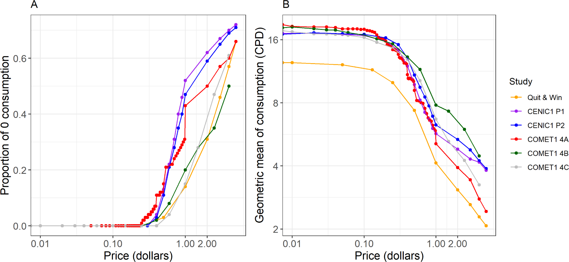
Summary plots of baseline cigarette purchase task data of six studies with price in logarithm scale. Panel A shows the proportion of zero consumption at each price for each study. Panel B shows the geometric mean of non-zero consumption, in cigarettes per day (CPD), at each price for each study.

3 |. A BAYESIAN HIERARCHICAL MODEL

In this section, we present a Bayesian hierarchical model for the analysis of individual participant data to synthesize CPT data from multiple studies. Our main goal was to estimate the combined group’s demand curve, and evaluate the between-study heterogeneity among study-specific demand curves. We extended the two-part mixed-effects model of Zhao et al.³⁰ for a single study to multiple studies using a Bayesian hierarchical model where between-study heterogeneity was appropriately considered.

Let us consider a meta-analysis of demand curves with a collection of K studies. Let Z_kij denote the binary outcome for cessation (i.e., Z = 1 if cessation, and Z = 0 if not) for subject i at the j^th unit price in study k, (i = 1, 2, ...,N_k, j = 1, 2, ..., J_k, k = 1, 2, ...,K), and without loss of generality, the J_k prices in study k are in increasing order. Let Y_ki (= 1, 2, ..., J_k) be the order of the unit prices at which the cessation happens, and X_ki represents the covariate vector for subject i in study k. Let p_kj denote the j^th unit price in study k. Let Q_kij > 0 represent a non-zero consumption value for subject i at the j^th unit price in study k.

Section 3.1 describes the first level of the proposed Bayesian hierarchical model, a within-study model. This level of model is a two-part mixed-effects model corresponding to the model introduced by Zhao et al.³⁰ Section 3.2 presents the second level model, a between-study level model used to properly consider between-study heterogeneity. Section 3.3 describes the prior specifications. Finally, Section 3.4 demonstrates the likelihood and posterior distribution of the proposed Bayesian hierarchical model.

3.1 |. Within-study model

The first part of the model introduced by Zhao et al.³⁰ is a logistic regression model used to estimate the probability of smoking cessation. As shown in Figure 1A, the study-specific probability of cessation does not have an S-shape for the entire range of pricing. Therefore, we considered linear splines for price in the logistic regression model to make the model more flexible. In this case, the model is linear to a function of the independent variable instead of the independent variable itself. Let h_j(X_ki) = P(Y_ki = j|Y_ki ≥ j, X_ki) be the hazard of cessation at the j^th price for people in study k with covariates X_ki, where P(·|·) denotes conditional probabilities. Let s index the subintervals of the spline method and S denote the total number of subintervals. Let p_s denote the unit price at the s^th knot (s = 1, 2, ..., S−1) for the linear spline method, and both S and p_s’s are predetermined. Let β_0k, β_10k, and β_1sk be study-specific intercepts and slopes for the s^th subinterval in study k (s = 1, 2, ..., S − 1, k = 1, 2, ...,K). Let β_x be the parameter vector for the covariates. The function f(·) is a proper function for price such as the shifted log transformation, log(price+0.001), and a_ki is the random intercept for subject i in study k. Therefore, the logistic model is represented as follows:

$$Z_{kij}~\text{Bernoulli}\left\{h_j\left({\mathit{X}}_{\mathit{k}\mathit{i}}\right)\right\},$$

and

$$\mathrm{logit}\left\{h_j\left({\mathbf{X}}_{\mathit{k}\mathit{i}}\right)\right\}={\beta }_{0k}+{\beta }_{10k}f\left(p_{kj}\right)+\sum _{s=1}^{S-1}{\beta }_{1sk}I\left(p_{kj}\ge p_s\right)\left\{f\left(p_{kj}\right)-f\left(p_s\right)\right\}+{\mathit{\beta }}_{\mathit{x}}^T{\mathit{X}}_{\mathit{k}\mathit{i}}+a_{ki}.$$ (2)

The second part of the model is about the relationship between the unit price and the hypothetical non-zero consumption (Q_kij). For the cigarette demand curve analysis, researchers assume that the relationship between the log-transformed positive response log(Q_kij) and price (p) is a nonlinear mixed-effects model.²⁴ Let μ_kij be the expected log-transformed demand and ϵ_kij be an independent error term which is distributed as N(0, σ²). Let logQ_0k be the study-specific intercept, while δ_k is the study-specific range of consumption in the log scale, which is usually a nuisance parameter and assumed to be fixed. Let γ_x and α_x be the parameter vectors for covariates. Let α_0k be a study-specific slope for price, b_ki and c_ki be the subject-specific random intercept and slope for subject i in study k. We assume that the random effects, (a_ki, b_ki, c_ki)^T, follow a multivariate normal distribution with mean 0 = (0, 0, 0)^T and variance-covariance matrix Σ, and that the random effects are independent. Then, the second-part model for j < Y_ki can be presented as:

$$\begin{gathered} \log \left(Q_{kij}\right)={\mu }_{kij}+{ϵ}_{kij}=\left(\log Q_{0k}+{\mathit{\gamma }}_{\mathit{x}}^T{\mathit{X}}_{\mathit{k}\mathit{i}}+b_{ki}\right)+{\delta }_k\left\{e^{-\left({\alpha }_{0k}+{\mathit{\alpha }}_{\mathit{x}}^T{\mathit{X}}_{\mathit{k}\mathit{l}}+c_{ki}\right)p_{kj}}-1\right\}+{ϵ}_{kij}, \\ {ϵ}_{kij}\stackrel{iid}{~}\text{N}\left(0,{\sigma }^2\right), \\ {\left(a_{ki},b_{ki},c_{ki}\right)}^T\stackrel{iid}{~}\text{MVN}(\mathbf{0},\mathrm{\Sigma }). \end{gathered}$$ (3)

3.2 |. Between-study model

The between-study model describes the heterogeneity across the studies. Let the collection of parameters for study k be denoted by θ_k = (β_0k, β_10k, β_1sk, logQ_0k, δ_k, α_0k), s = 1, 2, ..., S − 1, and assume that θ_k, k = 1, 2, ...., K, are independent. To account for between-study heterogeneity, we assume that the study-specific parameters follow normal distributions:

$${\beta }_{0k}\stackrel{iid}{~}\text{N}\left({\beta }_0,{\sigma }_{{\beta }_0}^2\right),$$

$${\beta }_{10k}\stackrel{iid}{~}\text{N}\left({\beta }_{10},{\sigma }_{{\beta }_{10}}^2\right),$$

$${\beta }_{1sk}\stackrel{iid}{~}\text{N}\left({\beta }_{1s},{\sigma }_{{\beta }_{1s}}^2\right),s=1,2,\dots ,S-1,$$

$$\log Q_{0k}\stackrel{iid}{~}\text{N}\left(\log Q_0,{\sigma }_{\log Q_0}^2\right)$$

$${\delta }_k\stackrel{iid}{~}\text{N}\left(\delta ,{\sigma }_{\delta }^2\right),\text{and}$$

$${\alpha }_{0k}\stackrel{iid}{~}\text{N}\left({\alpha }_0,{\sigma }_{{\alpha }_0}^2\right).$$

At the same time, we assume the parameter vectors for covariates (i.e., β_x, γ_x, and α_x) to be the same for all studies. We also assume the variance-covariance matrix for (a_ki, b_ki, c_ki)^T and the variance for ϵ (i.e., Σ and σ²) to be homogeneous for all studies.

3.3 |. Prior specifications

Let π(·) denote the probability density function of the priors for parameters, and let θ = (β₀, β₁₀, β_1s, logQ₀, δ, α₀) and $\mathit{\eta }=\left({\sigma }_{{\beta }_0},{\sigma }_{{\beta }_{10}},{\sigma }_{{\beta }_{1s}},{\sigma }_{\log Q_0},{\sigma }_{\delta },{\sigma }_{{\alpha }_0}\right),s=1,2,\dots ,S-1$. Then, the prior joint distribution of β₀, β₁₀, β_1s, logQ₀, δ, α₀, ${\sigma }_{{\beta }_0}$, ${\sigma }_{{\beta }_{10}}$, ${\sigma }_{{\beta }_{1s}}$, ${\sigma }_{\log Q_0}$, σ_δ, ${\sigma }_{{\alpha }_0}$, β_x, γ_x, α_x, δ, σ, and Σ can be expressed as:

$$\begin{gathered} \pi (\mathit{\theta },\mathit{\eta },{\mathit{\beta }}_{\mathit{x}},{\mathit{\gamma }}_{\mathit{x}},{\mathit{\alpha }}_{\mathit{x}},\delta ,\sigma ,\mathrm{\Sigma })=\pi ({\beta }_0)\pi ({\sigma }_{{\beta }_0})\pi ({\beta }_{10})\pi ({\sigma }_{{\beta }_{10}})\prod _{s=1}^{S-1}\left\{\pi ({\beta }_{1s})\pi ({\sigma }_{{\beta }_{1s}})\right\}\pi (\log Q_0)\pi ({\sigma }_{\log Q_0})\pi ({\alpha }_0)\pi ({\sigma }_{{\alpha }_0})\pi ({\mathit{\beta }}_{\mathit{x}})\pi ({\mathit{\gamma }}_{\mathit{x}})\pi ({\mathit{\alpha }}_{\mathit{x}}) \\ \pi (\delta )\pi ({\sigma }_{\delta })\pi (\sigma )\pi (\mathrm{\Sigma }). \end{gathered}$$

The Bayesian specification is completed with noninformative priors. As Gelman³⁹ and Ho et al.²⁵ noted, the priors for β₀, β₁₀, β_1s, β_x, logQ₀, γ_x, and δ (s = 1, 2, ..., S − 1) are normal priors with large variances, and uniform priors are used for ${\sigma }_{{\beta }_0}$, ${\sigma }_{{\beta }_{10}}$, ${\sigma }_{{\beta }_{1s}}$, ${\sigma }_{\log Q_0}$, σ_δ, α₀, α_x, ${\sigma }_{{\alpha }_0}$, and σ (s = 1, 2, ..., S − 1). In addition, the prior for Σ is specified to be Σ⁻¹ ~ Wishart(Ω, u).

3.4 |. Likelihood and posterior distribution

Finally, we present the likelihood and posterior distribution of the proposed Bayesian hierarchical model. Let Z and Q represent the vectors for the binary outcome for cessation and the hypothetical consumption, respectively. Through the Bayesian hierarchical model and priors that we specified, we can derive the likelihood as follows:

$$\begin{gathered} L\left[\mathit{Z},\log \mathit{Q}\mid \mathit{\theta },\mathit{\eta },{\mathit{\beta }}_{\mathit{x}},{\mathit{\gamma }}_{\mathit{x}},{\mathit{\alpha }}_{\mathit{x}},\sigma ,\mathrm{\Sigma }\right]=\prod _{k=1}^K[\prod _{i=1}^{N_k}\prod _{j=1}^{J_k}\left\{P\left(\log Q_{kij},z_{kij}\mid {\beta }_{0k},{\beta }_{10k},{\beta }_{1sk},\log Q_{0k},{\delta }_k,{\alpha }_{0k},{\mathit{\beta }}_{\mathit{x}},{\mathit{\gamma }}_{\mathit{x}},{\mathit{\alpha }}_{\mathit{x}},\sigma ,\mathrm{\Sigma }\right)\right\} \\ \times P\left({\beta }_{0k}\mid {\beta }_0,{\sigma }_{{\beta }_0}\right)\times P\left({\beta }_{10k}\mid {\beta }_{10},{\sigma }_{{\beta }_{10}}\right)\left\{\prod _{s=1}^{S-1}P\left({\beta }_{1sk}\mid {\beta }_{1s},{\sigma }_{{\beta }_{1s}}\right)\right\} \\ \times P\left({\delta }_k\mid \delta ,{\sigma }_{\delta }\right)P\left({\alpha }_{0k}\mid {\alpha }_0,{\sigma }_{{\alpha }_0}\right)P\left(\log Q_{0k}\mid \log Q_0,{\sigma }_{\log Q_0}\right)]. \end{gathered}$$

The P(·|·)’s are well defined likelihood functions, which can be found in Sections 3.1 and 3.2. Thus, the posterior distribution of β₀, ${\sigma }_{{\beta }_0}$, β₁₀, ${\sigma }_{{\beta }_{10}}$, β_1s, ${\sigma }_{{\beta }_{1s}}$ (s = 1, 2, ..., S − 1), logQ₀, ${\sigma }_{\log Q_0}$, δ, σ_δ, α₀, ${\sigma }_{{\alpha }_0}$, β_x, γ_x, α_x, σ, and Σ, given the observations, is proportional to:

$$P\left(\mathit{\theta },\mathit{\eta },{\mathit{\beta }}_{\mathit{x}},{\mathit{\gamma }}_{\mathit{x}},{\mathit{\alpha }}_{\mathit{x}},\sigma ,\mathrm{\Sigma }\mid \mathit{Z},\log \mathit{Q}\right)\propto L[\mathit{Z},\log \mathit{Q})\mid \mathit{\theta },\mathit{\eta },{\mathit{\beta }}_{\mathit{x}},{\mathit{\gamma }}_{\mathit{x}},{\mathit{\alpha }}_{\mathit{x}},\sigma ,\mathrm{\Sigma }]\times \pi \left(\mathit{\theta },\mathit{\eta },{\mathit{\beta }}_{\mathit{x}},{\mathit{\gamma }}_{\mathit{x}},{\mathit{\alpha }}_{\mathit{x}},\sigma ,\mathrm{\Sigma }\right).$$

With these assumptions and the model, we are able to do the posterior computation using the Markov chain Monte Carlo (MCMC) method, and the computation was carried out using the downloadable, free software JAGS (http://mcmc-jags.sourceforge.net) and the rjags package in R (http://www.r-project.org/). The computing code can be found in Section 4 of the Supplementary Materials. The posterior credible intervals (CI) for β₀, ${\sigma }_{{\beta }_0}$, β₁₀, ${\sigma }_{{\beta }_{10}}$, β_1s, ${\sigma }_{{\beta }_{1s}}$ (s = 1, 2, ..., S − 1), logQ₀, ${\sigma }_{\log Q_0}$, δ, σ_δ, α₀, ${\sigma }_{{\alpha }_0}$, β_x, γ_x, α_x, σ, and Σ can be obtained from the posterior distribution approximated by the MCMC samples.

4 |. RESULTS FOR THE CASE STUDY

For the motivating data example, baseline age, gender, and race for each subject were available and measured the same way for each study, based on which we created three indicator variables for Age ≤ 25, Gender = Male, and Race = Non-white as covariates in the model (i.e., X_ki = {I(Age_ki ≤ 25), I(Gender_ki = Male), I(Race_ki = Non-white)}^T). The Age variable was dichotomized at 25 based on the 31st tobacco-related Surgeon General’s report which defines youth with ages 12 through 17 and young adults with ages 18 through 25.⁴⁰ Therefore, the parameter vectors for the three covariates are β_x = (β₂, β₃, β₄)^T, γ_x = (γ₁, γ₂, γ₃)^T, and α_x = (α₁, α₂, α₃)^T. The number and location of knots are informed by Figure 1A, where we see a possible knot around unit price $1. Therefore, we chose S = 2 subintervals with one knot at unit price $1 for the linear spline method. We also observed from Figure 1A that there could be a separation between different studies’ observed zero consumption curves beyond the knot, but the proposed model allows study-specific spline term parameters (β_11k) to accommodate this between-study heterogeneity. Following Zhao et al.,³⁰ we used the shifted log transformation on price (i.e., f(x) = log(x + 0.001)). Before fitting the full model, the individual participant model was applied to the six studies. As the estimated δ’s were close to each other, in the case study, we set δ_k = δ for all k. The final two-part model for the motivating data example can be written as follows:

Part I model (for the binary cessation outcome):

$$\mathrm{logit}\left(h_j\left({\mathit{X}}_{\mathit{k}\mathit{i}}\right)\right)={\beta }_{0k}+{\beta }_{10k}\log \left(p_{kj}+0.001\right)+{\beta }_{11k}I\left(p_{kj}\ge 1\right)\left\{\log \left(p_{kj}+0.001\right)-\log (1.001)\right\}+{\mathit{\beta }}_{\mathit{x}}^T{\mathit{X}}_{\mathit{k}\mathit{i}}+a_{ki};$$

Part II model (for the continuous consumption outcome):

$$\log \left(Q_{kij}\right)={\mu }_{kij}+{ϵ}_{kij}=\left(\log Q_{0k}+{\mathit{\gamma }}_{\mathit{x}}^T{\mathit{X}}_{\mathit{k}\mathit{i}}+b_{ki}\right)+\delta \left\{e^{-\left({\alpha }_{0k}+{\mathit{\alpha }}_{\mathit{x}}^T{\mathit{X}}_{\mathit{k}\mathit{i}}+c_{ki}\right)p_{kj}}-1\right\}+{ϵ}_{kij}.$$

The priors used for the motivating data example are as follows^39,25: β₀, β₁₀, β₁₁, β₂, β₃, β₄ ~ N(0, 2²), logQ₀, γ₁, γ₂, γ₃, δ ~ N(0, 10⁶), α₀ ~ unif(0, 100), α₁, α₂, α₃ ~ unif(−10, 10), ${\sigma }_{{\beta }_0}$, ${\sigma }_{{\beta }_{10}}$, ${\sigma }_{{\beta }_{11}}$, ${\sigma }_{\log Q_0}$, ${\sigma }_{{\alpha }_0}$, σ ~ unif(0, 10) and Σ⁻¹ ~ Wishart(Ω, u) where $\mathrm{\Omega }=\left(\begin{array}{ccc}1& 0.1& 0.1\\ 0.1& 1& 0.1\\ 0.1& 0.1& 1\end{array}\right)$ and u = 3. We tried various prior distributions for α’s, including the normal priors used in a previous animal study of our group,²⁵ and the simulation results showed that the uniform prior was the most stable one among different priors. The prior distributions for variances were determined by following Gelman³⁹ where it was noted that prior distribution on a compact set (e.g., in the range [−A, A] for some large value of A) would lead to a posterior distribution depending strongly on the lower bound. Since our model was developed based on the model proposed by Zhao et al.,³⁰ we expected the estimated α₀ to be greater than 0, so the prior for α₀ was set to be uniform with a lower bound 0. For α_x, since we had no prior information for these parameters, we let the likelihood determine the values. So, we let α_x have uniform prior with a relatively large range (0, 100). Three chains were used, with each chain having 4,000 burn-in iterations and 10,000 MCMC samples.

Table 3 details the summarized result of the posterior sample distributions for all population-level parameters. The estimated curves for the two-part model are shown in Section 1 of the Supplementary Materials. Convergence diagnostics were conducted with the Gelman and Rubin convergence statistics⁴¹ with three chains. The GR diagnostics for θ and η are all close to 1 (i.e., ranging from 1.00 to 1.10). Based on the estimated regression coefficients for the three covariates reported in Table 3, younger ages were significantly related to a smaller intensity (estimated γ₁ = −0.18, 95% CI = [−0.24, −0.12]) and higher elasticity to price change because of a larger α value (estimated α₁ = 0.07, 95% CI = [0.02, 0.12]). Male gender was significantly related to higher intensity (estimated γ₂ = 0.05, 95% CI = [0.02, 0.08]). Non-white race was significantly related to a smaller intensity (estimated γ₃ = −0.25, 95% CI = [−0.29, −0.20]) and a lower hazard of cessation (estimated β₄ = −0.30, 95% CI = [−0.45, −0.12]).

TABLE 3.

Population-level parameter estimates based on the Bayesian hierarchical model for the motivating data set

Parameter	Posterior Median	Posterior Mean	MC SE	95% CI
Part I model parameters
β 0	−2.12	−2.10	0.42	(−2.89, −1.20)
${\sigma }_{{\beta }_0}$	0.82	0.94	0.46	(0.43, 2.15)
β 10	2.86	2.86	0.21	(2.45, 3.26)
${\sigma }_{{\beta }_{10}}$	0.20	0.26	0.27	(0.01, 0.92)
β 11	−2.05	−2.03	0.36	(−2.69, −1.26)
${\sigma }_{{\beta }_{11}}$	0.62	0.71	0.41	(0.23, 1.74)
β 2	0.01	0.01	0.09	(−0.16, 0.19)
β 3	0.09	0.09	0.07	(−0.05, 0.23)
β 4	−0.30	−0.30	0.08	(−0.45, −0.12)
Part II model parameters
α 0	0.50	0.50	0.07	(0.37, 0.65)
${\sigma }_{{\alpha }_0}$	0.12	0.14	0.07	(0.06, 0.32)
logQ0	2.99	2.99	0.10	(2.79, 3.19)
${\sigma }_{\log Q_0}$	0.19	0.22	0.11	(0.10, 0.50)
δ	3.20	3.20	0.03	(3.11, 3.24)
α 1	0.07	0.07	0.03	(0.02, 0.12)
α 2	−0.03	−0.03	0.02	(−0.08, 0.01)
α 3	−0.03	−0.03	0.02	(−0.06, 0.04)
γ 1	−0.17	−0.18	0.03	(−0.24, −0.12)
γ 2	0.06	0.05	0.02	(0.02, 0.08)
γ 3	−0.25	−0.25	0.02	(−0.29, −0.20)
σ	0.25	0.25	0.00	(0.25, 0.25)
Covariance matrix for (aki, dki, cki)
Σ[1,1]	1.25	1.32	0.26	(0.90, 1.91)
Σ[1,2]	−0.04	−0.04	0.02	(−0.07, −0.01)
Σ[1,3]	0.20	0.21	0.01	(0.18, 0.24)
Σ[2,1]	−0.04	−0.04	0.02	(−0.07, −0.01)
Σ[2,2]	0.33	0.33	0.01	(0.32, 0.35)
Σ[2,3]	0.07	0.07	0.00	(0.06, 0.08)
Σ[3,1]	0.20	0.21	0.01	(0.18, 0.24)
Σ[3,2]	0.07	0.07	0.00	(0.06, 0.08)
Σ[3,3]	0.15	0.15	0.01	(0.14, 0.16)

Note. MC SE: Monte Carlo standard error; CI: credible interval.

Of note, we examined models (not shown) with different functional forms of the continuous age, the scaled age defined as (Age − min(Age))/(max(Age) − min(Age)) and log(Age) and compared them with the model with binary age, and found that the binary age model had the smallest DIC. We did not consider cutoff other than 25 years for the binary age due to the concern of multiple testing or polynomials due to the difficulty in result interpretation.

In addition to the one-step approach of the proposed Bayesian hierarchical model, we also tried a two-step approach by estimating the study-level parameters for each study separately and then using the random-effects meta-analysis method to calculate the population-level parameters. Table 4 shows a comparison between the results of the one-step and two-step approaches for both the study-level parameters (β_0k, β_10k, β_11k, logQ_0k, and α_0k) and population-level parameters (β₀, β₁₀, β₁₁, logQ₀, and α₀). The forest plots for these parameters for both the one-step and two-step approaches are shown in Figure 2. For the study-level parameters, the estimates of the one-step approach of the proposed Bayesian hierarchical model shrink toward the population-level parameters estimates when compared to the estimates of the two-step approach. This figure also shows different levels of between-study heterogeneity in model parameters. A prominent result is the parameter of logQ_0k in Figure 2D, which possibly reflects the lower amount of use, hence lower demand of cigarettes in the college/university population of the Quit & Win study compared to the smoking populations in the other five studies. The particularly noticeable shrinkage in α_0k for COMET1 4A as shown in Figure 2E indicates that the population in COMET 4A may be more sensitive in the amount of consumption to price than the rest of the population, and the small sample size (the smallest among the 6 studies) may also contribute to the large shrinkage.

TABLE 4.

Study-and population-level parameter estimates for β₀, β₁₀, β₁₁, logQ₀, and α₀ using both one-step and two-step approaches.

Project	β0k (MC SE)	β10k (MC SE)	β11k (MC SE)	logQ0k (MC SE)	α0k (MC SE)
Quit & Win One-step approach	−2.56 (0.16)	2.83 (0.18)	−1.58 (0.21)	2.69 (0.03)	0.44 (0.04)
Two-step approach	−2.79 (0.19)	2.79 (0.22)	−1.40 (0.24)	2.70 (0.03)	0.37 (0.02)
CENIC1 P1 One-step approach	−1.28 (0.11)	2.77 (0.18)	−2.67 (0.21)	3.06 (0.03)	0.56 (0.03)
Two-step approach	−1.50 (0.12)	2.28 (0.16)	−2.40 (0.19)	2.96 (0.04)	0.52 (0.04)
CENIC1 P2 One-step approach	−1.49 (0.09)	2.79 (0.18)	−2.53 (0.18)	3.03 (0.02)	0.48 (0.03)
Two-step approach	−1.50 (0.09)	2.24 (0.12)	−2.20 (0.17)	2.98 (0.02)	0.51 (0.02)
COMET1 4A One-step approach	−2.97 (0.20)	2.98 (0.23)	−1.85 (0.33)	3.12 (0.05)	0.67 (0.04)
Two-step approach	−2.79 (0.23)	2.55 (0.27)	−1.64 (0.38)	3.22 (0.06)	1.38 (0.06)
COMET1 4B One-step approach	−2.43 (0.21)	2.81 (0.23)	−2.16 (0.31)	3.01 (0.05)	0.43 (0.05)
Two-step approach	−3.43 (0.60)	3.49 (0.56)	−2.12 (0.63)	3.02 (0.06)	0.65 (0.16)
COMET1 4C One-step approach	−2.41 (0.20)	3.07 (0.32)	−1.70 (0.39)	3.03 (0.04)	0.44 (0.04)
Two-step approach	−2.23 (0.30)	3.38 (0.48)	−1.94 (0.57)	3.05 (0.05)	0.35 (0.02)
Summary One-step approach	−2.10 (0.42)	2.86 (0.21)	−2.03 (0.36)	2.99 (0.10)	0.50 (0.07)
Two-step approach	−2.22 (0.19)	2.72 (0.10)	−2.05 (0.14)	2.99 (0.04)	0.56 (0.08)

Note. MC SE: Monte Carlo standard error.

FIGURE 2.

The forest plots for the estimated study- and population-level parameters β_0k (Panel A), β_10k (Panel B), β_11k (Panel C), logQ_0k (Panel D), and α_0k (Panel E) using both the one-step (black horizontal bars) and two-step approaches (gray horizontal bars). The vertical lines represent the population-level parameter estimates (solid line for one-step and dash line for two-step approach).

With the Bayesian hierarchical approach, we can calculate the synthetical demand curve using the MCMC sampling method. With the Bayesian model, any function of parameters can be easily obtained with multiplicity of posterior samples, and the problem of multiple comparison disappear entirely.⁴² Therefore, we calculated the RRE indices, intensity (Q₀), Omax, Pmax, and α using posterior samples and presented the results in Table 5. The contrasts between subgroups in terms of the intensity and α values are consistent with the findings from the regression coefficients for the covariates reported in Table 3: older ages, male gender, and white race were associated with higher intensities; and younger ages were associated with higher sensitivity to price. In addition, older ages, male gender, and white race also showed positive correlations with Omax and Pmax.

TABLE 5.

Estimated relative reinforcing efficacy indices for populations stratified by age, gender, and race

Covariate values	Intensity (MC SE)	Omax (MC SE)	Pmax (MC SE)	α (MC SE)
Age ≤ 25, Gender = Male, Race = White	17.62 (1.85)	4.01 (0.71)	0.46 (0.07)	0.55 (0.07)
Age ≤ 25, Gender = Male, Race = Non-white	13.76 (1.47)	3.33 (0.64)	0.48 (0.08)	0.52 (0.07)
Age ≤ 25, Gender = Female, Race = White	16.69 (1.75)	3.59 (0.61)	0.43 (0.06)	0.58 (0.07)
Age ≤ 25, Gender = Female, Race = Non-white	13.04 (1.38)	2.97 (0.55)	0.46 (0.07)	0.55 (0.07)
Age > 25, Gender = Male, Race = White	21.06 (2.16)	5.59 (1.27)	0.53 (0.11)	0.47 (0.07)
Age > 25, Gender = Male, Race = Non-white	16.45 (1.70)	4.69 (1.28)	0.57 (0.15)	0.44 (0.07)
Age > 25, Gender = Female, Race = White	19.95 (2.07)	4.96 (1.00)	0.50 (0.09)	0.50 (0.07)
Age > 25, Gender = Female, Race = Non-white	15.58 (1.62)	4.14 (0.94)	0.53 (0.11)	0.47 (0.08)

Note. MC SE: Monte Carlo standard error; α: measure of reinforcing strength.

5 |. SIMULATION

For the simulation study, we used S = 2 subintervals with 1 knot at unit price $1 for the linear spline method and the transformation function for price, f(x) = log(x + 0.001) as in the motivating data set. We did the simulation 1000 times, and for each simulation, we generated 10 or 5 studies and 200 or 100 subjects for each study to demonstrate the performance of the proposed Bayesian hierarchical model. For each subject, the cigarette consumption was measured at 21 various unit prices from $0 to $5 (i.e., $0, $0.02, $0.05, $0.1, $0.2, $0.3, $0.4, $0.5, $0.6, $0.7, $0.8, $0.9, $1, $1.5, $2, $2.5, $3, $3.5, $4, $4.5, and $5). The true values for the parameters were set as: β₀ = −2, ${\sigma }_{{\beta }_0}=1$, β₁₀ = 2.5, ${\sigma }_{{\beta }_{10}}=0.4$, β₁₁ = −1.4, ${\sigma }_{{\beta }_{11}}=0.4$, logQ₀ = 2.5, ${\sigma }_{\log Q_0}=1.1$, α₀ = 4, ${\sigma }_{{\alpha }_0}=1$, δ = 2.8, and σ = 0.06. The random effects for each subject were generated from a multivariate normal distribution:

$$\left(\begin{array}{c}{a}_{ki}\\ b_{ki}\\ c_{ki}\end{array}\right)\stackrel{iid}{~}\text{N}(\left(\begin{array}{c}0\\ 0\\ 0\end{array}\right),\left(\begin{array}{ccc}0.5& 0.1& 0.1\\ 0.1& 0.5& 0.1\\ 0.1& 0.1& 0.5\end{array}\right)).$$

The prior distributions we used for the simulation are: β₀ ~ N(0, 2²), β₁₀ ~ N(0, 2²), β₁₁ ~ N(0, 2²), logQ₀ ~ N(0, 10⁶), α₀ ~ unif(0, 100), δ ~ N(0, 10⁶), ${\sigma }_{{\beta }_0}~\mathrm{unif}(0,10)$, ${\sigma }_{{\beta }_{10}}~\mathrm{unif}(0,10)$, ${\sigma }_{{\beta }_{11}}~\mathrm{unif}(0,10)$, ${\sigma }_{{\alpha }_0}~\mathrm{unif}(0,10)$, ${\sigma }_{\log Q_0}~\mathrm{unif}(0,10)$, and σ ~ unif(0, 10). For the random effects’s variance, we used ${\mathrm{\Sigma }}^{-1}~\text{Wishart}(\left(\begin{array}{ccc}1& 0.1& 0.1\\ 0.1& 1& 0.1\\ 0.1& 0.1& 1\end{array}\right),3)$. The summary of the simulation results for the proposed Bayesian hierarchical model, including true value, posterior mean, Monte Carlo standard error (MC SE), relative bias, and 95% coverage rate, is shown in Table 6. The posterior means from our proposed model are close to their true values with small relative bias and satisfactory 95% coverage rate. The estimates for the standard deviations (i.e., ${\sigma }_{{\beta }_0}$, ${\sigma }_{{\beta }_{10}}$, ${\sigma }_{{\beta }_{11}}$, ${\sigma }_{\log Q_0}$, and ${\sigma }_{{\alpha }_0}$) also have around 95% coverage rates and small biases. Also, we found that under our simulation scenarios, the bias for β₀ is relatively high compared with the other parameters when the number of study is small, while the coverage rate does not change much with the number of studies. This indicates that the posterior distribution for this parameter might be skewed with a small number of studies. With the hierarchical model, we were able to calculate both the study- and population-level parameters in a one-step approach. As compared with the two-step random-effects meta-analysis approach, one of the advantages of the proposed one-step Bayesian hierarchical model is that once a posterior distribution of a parameter is obtained from Bayesian methods, one can directly provide information such as the posterior probability that the parameter is greater than certain values, which is difficult to obtain using the frequentist two-step approach. Further simulations including simulation for the two-step approach and the sensitivity analysis for both one-step and two-step approach were also conducted. Details can be found in Section 3 of the Supplementary Materials.

TABLE 6.

Simulation result

Size	Parameter	True Value	Posterior Mean	MC SE	Relative Bias	95% Coverage Rate
5 × 100	β 0	−2	−1.80	0.68	0.10	0.97
	β 10	2.5	2.47	0.45	0.01	0.99
	β 11	−1.4	−1.33	0.52	0.05	0.99
	logQ0	2.5	2.39	0.91	0.04	0.98
	α 0	4	4.01	0.74	0.00	0.97
	δ	2.8	2.80	0.01	0.00	0.95
10 × 100	β 0	−2	−1.94	0.38	0.03	0.97
	β 10	2.5	2.52	0.25	0.01	0.97
	β 11	−1.4	−1.38	0.29	0.01	0.96
	logQ0	2.5	2.46	0.43	0.02	0.97
	α 0	4	4.00	0.38	0.00	0.96
	δ	2.8	2.81	0.01	0.00	0.94
5 × 200	β 0	−2	−1.77	0.68	0.12	0.97
	β 10	2.5	2.46	0.40	0.02	0.98
	β 11	−1.4	−1.36	0.44	0.03	0.99
	logQ0	2.5	2.47	0.84	0.01	0.98
	α 0	4	4.00	0.73	0.00	0.98
	δ	2.8	2.81	0.01	0.00	0.94
10 × 200	β 0	−2	−1.92	0.38	0.04	0.96
	β 10	2.5	2.52	0.22	0.01	0.97
	β 11	−1.4	−1.39	0.24	0.01	0.97
	logQ0	2.5	2.49	0.42	0.00	0.96
	α 0	4	3.99	0.38	0.01	0.96
	δ	2.8	2.81	0.00	0.00	0.92

Note. Size: number of studies × number of subjects per study; MC SE: Monte Carlo standard error; Relative Bias = (estimate − true)∕true.

6 |. DISCUSSION

The exponential demand curve²⁴ has been widely used for analyzing data generated from the CPT.⁴³ Zhao et al.³⁰ proposed the two-part mixed-effects model to appropriately consider cessation without arbitrarily imputing values for zeros. In this paper, we extended the two-part mixed-effects model proposed by Zhao et al.³⁰ to a Bayesian hierarchical model for meta-analysis of the CPT data collected in six studies. For the Bayesian hierarchical model, we assumed that the study-level parameters were heterogeneous among studies and that the true parameters were samples from normal distributions, which is commonly used in Bayesian analysis with random effects.⁴⁴ In future research, we can consider other distributions (e.g., multivariate t distribution). This work is meant to be a proof of concept for demonstrating the utility of the Bayesian framework for the analysis of complex data, but we acknowledge that the proposed model contains a substantial number of parameters and may require the study of its sensitivity to choices of priors and other features. Compared with the conventional random-effects meta-analysis method, the Bayesian hierarchical model can estimate both study- and population-level parameters simultaneously. At the same time, the estimates and 95% CIs of the commonly used RRE indices, Omax and Pmax, which are not directly from the model parameters, can be obtained easily with posterior samples from MCMC method.

To make the trend of the hazard of cessation more flexible, we included linear spline terms on the top of the transformed price in the proposed Part I model. As demonstrated with our motivating data example, the number of sub-intervals and the location of knots can be determined empirically by examining the plot of the proportion of zero consumption. Other more sophisticated spline functions may be considered if the data suggest so and can be accommodated in our proposed model. Also, as demonstrated in Zhao et al.,³⁰ other functional forms of price may be chosen if supported by residual diagnosis results. We also want to mention that as a byproduct of the proposed model, we can derive the formula for the cumulative probability of zeros from the hazard of cessation for combinations of covariate values (shown in Appendix A). One possible model diagnosis method could be comparing the estimated cumulative probability of zeros with the observed proportions in addition to the comparison between observed demand curves for individuals and the estimated demand curve by study (as shown in Figure S2 in the Supplementary Materials, Section 2).

There are two statistical approaches for conducting the IPD meta-analyses: one-step and two-step approach. The one-step approach is to estimate the study-level and overall parameters simultaneously, while the two-step approach is to estimate the study-level parameters separately, then use traditional meta-analysis methods to combine these results. In this paper, we demonstrated both one-step and two-step approaches and compared their results. The one-step approach is more efficient, especially when estimating population-level parameters. The overall results for the two approaches are similar, and the study-level parameter estimates shrink towards the population-level estimates.^45,46

In conclusion, in this study, we evaluated the performance of the proposed Bayesian hierarchical model for meta-analysis of demand curves. The proposed Bayesian hierarchical model allows the meta-analysis of multiple purchase task data within one step. Although we only implemented the model on CPT data in this paper, the proposed model can be used for purchase task data of other products such as e-cigarettes.

APPENDIX

APPENDIX A. DERIVING THE CUMULATIVE PROBABILITY OF CESSATION

The cumulative probability of cessation can be expressed as a function of hazards of cessation at a sequence of prices as follows:

$$\begin{gathered} P\left(Y_{ki}\le j\mid {\mathit{X}}_{\mathit{k}\mathit{i}}\right)=1-P\left(Y_{ki}\ge j+1\mid {\mathit{X}}_{\mathit{k}\mathit{i}}\right) \\ =1-P\left(Y_{ki}\ge 1,Y_{ki}\ge 2,\dots ,Y_{ki}\ge j+1\mid {\mathit{X}}_{\mathit{k}\mathit{i}}\right) \\ =1-\prod _{t=1}^{j}P\left(Y_{ki}\ge t+1\mid Y_{ki}\ge t,{\mathit{X}}_{\mathit{k}\mathit{i}}\right) \\ =1-\prod _{t=1}^j\left\{1-P\left(Y_{ki}=t\mid Y_{ki}\ge t,{\mathit{X}}_{\mathit{k}\mathit{i}}\right)\right\} \\ =1-\prod _{t=1}^j\left\{1-h_t\left({\mathit{X}}_{\mathit{k}\mathit{i}}\right)\right\}. \end{gathered}$$

References

- 1.Borenstein M, Hedges LV, Higgins JPT, Rothstein HR. Introduction to Meta-Analysis. New York, NY: John Wiley & Sons; 2009. [Google Scholar]
- 2.Lin L, Chu H, Quantifying publication bias in meta-analysis. Biometrics. 2018;74(3): 785–794. [DOI] [PMC free article] [PubMed] [Google Scholar]
- 3.Hong C, Salanti G, Morton SC, Riley RD, Chu H, Kimmel SE, Chen Y. Testing small study effect in multivariate meta-analysis. Biometrics. 2020;76(4):1240–1250. [DOI] [PMC free article] [PubMed] [Google Scholar]
- 4.Dersimonian R, Laird N. Meta-analysis in clinical trials. Control Clin Trials. 1986;7(3):177–188. [DOI] [PubMed] [Google Scholar]
- 5.Orlitzky M, Schmidt FL, Rynes SL. Corporate social and financial performance: a meta-analysis. Organ Stud. 2003;24(3):403–441. [Google Scholar]
- 6.Sullivan PF, Neale MC, Kendler KS. Genetic epidemiology of major depression: review and meta-analysis. Am J Psychiatry. 2000;157(10):1552–1562. [DOI] [PubMed] [Google Scholar]
- 7.Riley RD, Lambert PC, Abo-Zaid G. Meta-analysis of individual participant data: rationale, conduct, and reporting. BMJ. 2010;340:c221. 10.1136/bmj.c221. [DOI] [PubMed] [Google Scholar]
- 8.Stewart LA, Clarke M, Rovers M, et al. Preferred reporting items for systematic review and meta-analyses of individual participant data: the PRISMA-IPD statement. JAMA. 2015;313(16):1657–1665. [DOI] [PubMed] [Google Scholar]
- 9.Riley RD, Price MJ, Jackson D, et al. Multivariate meta-analysis using individual participant data. Res Synth Methods. 2015;6(2):157–174. [DOI] [PMC free article] [PubMed] [Google Scholar]
- 10.Riley RD, Lambert PC, Staessen JA, et al. Meta-analysis of continuous outcomes combining individual patient data and aggregate data. Stat Med. 2008;27(11):1870–1893. [DOI] [PubMed] [Google Scholar]
- 11.Riley RD, Dodd SR, Craig JV, Thompson JR, Williamson PR. Meta-analysis of diagnostic test studies using individual patient data and aggregate data. Stat Med. 2008;27(29):6111–6136. [DOI] [PubMed] [Google Scholar]
- 12.Bender R, Friede T, Koch A, et al. Methods for evidence synthesis in the case of very few studies. Res Synth Methods. 2018;9(3):382–392. [DOI] [PMC free article] [PubMed] [Google Scholar]
- 13.Rice K, Higgins JPT, Lumley T. A re-evaluation of fixed effect(s) meta-analysis. J R Stat Soc Ser A Stat Soc. 2018;181(1):205–227. [Google Scholar]
- 14.Higgins JP, Thompson SG, Spiegelhalter DJ. A re-evaluation of random-effects meta-analysis. J R Stat Soc Ser A Stat Soc. 2009;172(1):137–159. [DOI] [PMC free article] [PubMed] [Google Scholar]
- 15.Tudur SC, Marcucci M, Nolan SJ, et al. Individual participant data meta-analyses compared with meta-analyses based on aggregate data. Cochrane Database Syst Rev. 2016;9(9):MR000007. [DOI] [PMC free article] [PubMed] [Google Scholar]
- 16.Cooper H, Patall EA. The relative benefits of meta-analysis conducted with individual participant data versus aggregated data. Psychol Methods. 2009;14(2):165–176. [DOI] [PubMed] [Google Scholar]
- 17.Simmonds MC, Higginsa JPT, Stewartb LA, Tierneyb JF, Clarke MJ, Thompson SG. Meta-analysis of individual patient data from randomized trials: a review of methods used in practice. Clinical Trials. 2005;2(3):209–217. [DOI] [PubMed] [Google Scholar]
- 18.Zvorsky I, Nighbor TD, Kurti AN, et al. Sensitivity of hypothetical purchase task indices when studying substance use: A systematic literature review. Prev Med. 2019. Nov;128:105789. 10.1016/j.ypmed.2019.105789. [DOI] [PMC free article] [PubMed] [Google Scholar]
- 19.Griffiths RR, Brady JV, Bradford LD. Predicting the abuse liability of drugs with animal drug self-administration procedures: psychomotor stimulants and hallucinogens. Advances in behavioral pharmacology. 1979;2:163–208. [Google Scholar]
- 20.Katz JL. Models of relative reinforcing efficacy of drugs and their predictive utility. Behav Pharmacol. 1990;1(4):283–301. [DOI] [PubMed] [Google Scholar]
- 21.Jacobs EA, Bickel WK. Modeling drug consumption in the clinic using simulation procedures: demand for heroin and cigarettes in opioid-dependent outpatients. Exp Clin Psychopharmacol. 1999;7(4):412–426. [DOI] [PubMed] [Google Scholar]
- 22.Hursh SR. Economic concepts for the analysis of behavior. J Exp Anal Behav. 1980;34(2):219–238. [DOI] [PMC free article] [PubMed] [Google Scholar]
- 23.Hursh SR, Raslear TG, Shurtleff D, Bauman R, Simmons L. A cost-benefit analysis of demand for food. J Exp Anal Behav. 1988;50(3):419–440. [DOI] [PMC free article] [PubMed] [Google Scholar]
- 24.Hursh SR, Silberberg A. Economic demand and essential value. Psychol Rev. 2008;115(1):186–198. [DOI] [PubMed] [Google Scholar]
- 25.Ho Y, Vo TN, Chu H, LeSage MG, Luo X, Le C. A Bayesian hierarchical model for demand curve analysis. Stat Methods Med Res. 2018;27(8):2401–2412. [DOI] [PubMed] [Google Scholar]
- 26.Koffarnus MN, Hall A, Winger G. Individual differences in rhesus monkeys’ demand for drugs of abuse. Addict Biol. 2012;17(5):887–896. [DOI] [PMC free article] [PubMed] [Google Scholar]
- 27.Koffarnus MN, Franck CT, Stein JS, Bickel WK. A modified exponential behavioral economic demand model to better describe consumption data. Exp Clin Psychopharmacol. 2015;23(6):504–512. [DOI] [PMC free article] [PubMed] [Google Scholar]
- 28.Galuska CM, Banna KM, Willse LV, Yahyavi-Firouz-Abadi N, See RE. A comparison of economic demand and conditioned-cued reinstatement of methamphetamine-seeking or food-seeking in rats. Behav Pharmacol. 2011;22(4):312–323. [DOI] [PMC free article] [PubMed] [Google Scholar]
- 29.MacKillop J, Few LR, Murphy JG, Wier LM, Acker J, Murphy C, Stojek M, Carrigan M, Chaloupka F. High-resolution Behavioral Economic Analysis of Cigarette Demand to Inform Tax Policy. Addiction. 2012;107(12):2191–2200. [DOI] [PMC free article] [PubMed] [Google Scholar]
- 30.Zhao T, Luo X, Chu H, Le C, Epstein L, Thomas JL. A two-part mixed effects model for cigarette purchase task data. J Exp Anal Behav. 2016;106(3):242–253. [DOI] [PMC free article] [PubMed] [Google Scholar]
- 31.Hursh SR. Behavioral economics of drug self-administration and drug abuse policy. J Exp Anal Behav. 1991;56(2):377–393. [DOI] [PMC free article] [PubMed] [Google Scholar]
- 32.Hursh SR, Winger G. Normalized demand for drugs and other reinforcers. J Exp Anal Behav. 1995;64(3):373–384. [DOI] [PMC free article] [PubMed] [Google Scholar]
- 33.Thomas JL, Luo X, Bengtson J, et al. Enhancing Quit & Win contests to improve cessation among college smokers: a randomized clinical trial. Addiction. 2015;111(2):331–339. [DOI] [PMC free article] [PubMed] [Google Scholar]
- 34.Donny EC, Denlinger RL, Tidey JW, et al. Randomized trial of reduced-nicotine standards for cigarettes. N Engl J Med. 2015;373(14):1340–1349. [DOI] [PMC free article] [PubMed] [Google Scholar]
- 35.Hatsukami DK, Luo X, Jensen JA, et al. Effect of immediate vs gradual reduction in nicotine content of cigarettes on biomarkers of smoke exposure: a randomized clinical trial. JAMA. 2018;320(9):880–891. [DOI] [PMC free article] [PubMed] [Google Scholar]
- 36.Meier E, Lindgren BR, Anderson A, et al. A randomized clinical trial of snus examining the effect of complete vs. partial cigarette substitution on smoking-related behaviors, and biomarkers of exposure. Nicotine Tob Res. 2020;22(4):473–481. [DOI] [PMC free article] [PubMed] [Google Scholar]
- 37.Hatsukami DK, Meier E, Lindgren BR, Anderson A, Reisinger SA, Norton KJ, Strayer L, Jensen JA, Dick L, Murphy SE, Carmella SG, Tang M-K, Chen M, Hecht SS, O’connor RJ, Shields PG. A randomized clinical trial examining the effects of instructions for electronic cigarette use on smoking-related behaviors and biomarkers of exposure. Nicotine Tob Res. 2020;22(9):1524–1532. [DOI] [PMC free article] [PubMed] [Google Scholar]
- 38.Smith TT, Cassidy RN, Tidey JW, Luo X, Le C, Hatsukami DK, Donny Ec. Impact of smoking reduced nicotine content cigarettes on sensitivity to cigarette price: further results from a multi-site clinical trial. Addiction. 2017;112(2):349–359. [DOI] [PMC free article] [PubMed] [Google Scholar]
- 39.Gelman A Prior distributions for variance parameters in hierarchical models (Comment on Article by Browne and Draper). Bayesian Anal. 2006;1(3):515–534. [Google Scholar]
- 40.Preventing Tobacco Use Among Youths, Surgeon General fact sheet. https://www.hhs.gov/surgeongeneral/reports-and-publications/tobacco/preventing-youth-tobacco-use-factsheet/index.htm. June 6, 2017. Accessed April 18, 2020.
- 41.Gelman A, Rubin DB. Inference from iterative simulation using multiple sequences. Stat Sci. 1993;7(4):457–472. [Google Scholar]
- 42.Gelman A, Hill J, Yajima M. Why We (Usually) Don’t Have to Worry About Multiple Comparisons. Journal of Research on Educational Effectiveness. 2012;5(2):189–211. [Google Scholar]
- 43.Murphy JG, Mackillop J, Tidey JW, Brazil LA, Colby SM. Validity of a demand curve measure of nicotine reinforcement with adolescent smokers. Drug Alcohol Depend. 2011;113(2–3):207–214. [DOI] [PMC free article] [PubMed] [Google Scholar]
- 44.Carlin BP, Louis TA. Bayesian methods for data analysis, 3rd ed. Chapman & Hall/CRC; 2009. [Google Scholar]
- 45.Burke DL, Ensor J, Riley RD. Meta-analysis using individual participant data: one-stage and two-stage approaches, and why they may differ. Stat Med. 2016;36(5):855–875. [DOI] [PMC free article] [PubMed] [Google Scholar]
- 46.Debray TPA, Moons KGM, Abo-Zaid GMA, Koffijberg H, Riley RD. Individual Participant Data Meta-Analysis for a Binary Outcome: One-Stage or Two-Stage? PLoS One. 2013;8(4):e60650. [DOI] [PMC free article] [PubMed] [Google Scholar]
Associated Data
This section collects any data citations, data availability statements, or supplementary materials included in this article.