Integrating neuroimaging and gene expression data using the imaging transcriptomics toolbox

Summary

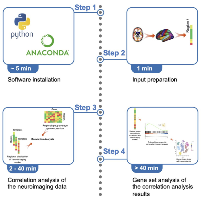
The integration of neuroimaging and transcriptomics data, Imaging Transcriptomics, is becoming increasingly popular but standardized workflows for its implementation are still lacking. We describe the Imaging Transcriptomics toolbox, a new package that implements a full imaging transcriptomics pipeline using a user-friendly, command line interface. This toolbox allows the user to identify patterns of gene expression which correlates with a specific neuroimaging phenotype and perform gene set enrichment analyses to inform the biological interpretation of the findings using up-to-date methods.

For complete details on the use and execution of this protocol, please refer to Martins et al. (2021).

Graphical abstract

Highlights

• •Protocol for using the Imaging Transcriptomics toolbox
• •Identifies transcriptomic correlates of neuroimaging data
• •Performs gene enrichment analysis to contextualize findings
• •Standardized and user-friendly pipeline using robust statistics

The integration of neuroimaging and transcriptomics data, Imaging Transcriptomics, is becoming increasingly popular but standardized workflows for its implementation are still lacking. We describe the Imaging Transcriptomics toolbox, a new package that implements a full imaging transcriptomics pipeline using a user-friendly, command line interface. This toolbox allows the user to identify patterns of gene expression which correlates with a specific neuroimaging phenotype and perform gene set enrichment analyses to inform the biological interpretation of the findings using up-to-date methods.

Before you begin

This toolbox allows the user to identify patterns of gene expression which correlates with a specific neuroimaging phenotype and perform gene set enrichment analyses to inform the biological interpretation of the findings using up-to-date methods.

This section includes all necessary steps to setup a dedicated python environment and install the Imaging Transcriptomics toolbox.

Anaconda python environment

Timing: < 10 min

The imaging transcriptomics package works in Windows and Unix systems (Mac OSX, Linux) with Python 3 (>=3.6). To run the script or use the library without the risk of dependencies conflicts with other scripts or libraries, we recommend installing everything in a dedicated Anaconda environment. The environment hereafter installed, will occupy about 1.1 GB of hard drive space (on a MacBook Pro with 1.4 GHz Quad-Core Intel Core i5 processor and macOS Big Sur). The creation of a dedicated environment allows the user to avoid the accidental generation of conflicts with other software or Python versions.

Note: The occupied space might slightly vary between different systems (i.e., macOS, Linux, Windows) due to the internal filesystem design.

• 1.Anaconda can be downloaded from https://www.anaconda.com/products/individual and installed following the specific instructions for individual computer specifications.
• 2.Once Anaconda is installed restart any open terminal and create a dedicated environment using Python (version 3.7) and pip using the following command:

> conda create --name transcriptomics python=3.7 pip

Follow the prompted instructions until the environment gets successfully created, for more details on the creation of Anaconda environments please refer to the official documentation of anaconda (https://docs.conda.io/projects/conda/en/latest/user-guide/tasks/manage-environments.html).

• 3.Activate your newly created Anaconda environment by typing:

> conda activate transcriptomics

Before you proceed, make sure that you are in the correct environment (troubleshooting 1).

• 4.We will now install the ENIGMA Toolbox (https://github.com/MICA-MNI/ENIGMA), a package released by the ENIGMA consortium that contains plotting functions used by the Imaging Transcriptomics toolbox to create some plots. To install the ENIGMA Toolbox, run the following commands:

> git clone https://github.com/MICA-MNI/ENIGMA.git

> cd ENIGMA

> python setup.py install

Note: Some errors may appear during the installation of the toolbox, to resolve them please refer to troubleshooting 4.

• 5.The last pre-requisite before installing the package is the installation of the pypls library to perform partial least square regression (PLS). This can be done using the following command:

> pip install -e git+https://github.com/netneurolab/pypyls.git/#egg=pyls

CRITICAL: Do not install pyls from the python package manager (i.e., Pypi), since that package performs different tasks.

Installation

Timing: 1 min

After the creation of the dedicated environment and installing all the dependencies that can’t be installed automatically, here we will install the core toolbox with its python dependencies. This will make available two scripts, one for the correlation analysis between neuroimaging data and gene expression and one for to perform gene set enrichment analysis (GSEA).

• 6.To install the Imaging Transcriptomic toolbox, comprising of the python library and command line script, run the following command from your terminal:

> pip install imaging-transcriptomics

After the process is complete, you can check if the installation was successful by typing the following command in the terminal:

> imagingtranscriptomics --help

Or by typing:

> imt_gsea --help

With both the previous commands, if successful, the help for each of the scripts will be displayed.

Key resources table

REAGENT or RESOURCE	SOURCE	IDENTIFIER
Deposited data
Gene expression data from human brain tissues	Allen Human Brain Atlas (AHBA)	http://human.brain-map.org/
Single cell RNA-seq data	(Lake et al., 2018)	NA
Software and algorithms
MATLAB	(MATLAB, 2020)	https://uk.mathworks.com/
FMRIB Software Library (FSL)	(Jenkinson et al., 2012; Smith et al., 2004; Woolrich et al., 2009)	https://fsl.fmrib.ox.ac.uk/fsl/fslwiki/
Anaconda	Anaconda Inc.	https://www.anaconda.com/products/individual
Abagen toolbox	(Arnatkevičiūtė et al., 2019; Hawrylycz et al., 2012; Markello et al., 2021)	https://github.com/netneurolab/abagen (https://doi.org/10.5281/zenodo.5129257)
Alleninf	(Gorgolewski et al., 2014)	https://github.com/chrisfilo/alleninf
ENIGMA Toolbox	(Larivière et al., 2021)	https://enigma-toolbox.readthedocs.io/en/latest/index.html
Netneurotools python library	Network Neuroscience Lab, Brain Imaging Centre, McGill University	https://github.com/netneurolab/netneurotools
Gseapy python library	(Fang, 2020)	https://github.com/zqfang/GSEApy
The Imaging Transcriptomics Toolbox	(Giacomel et al., 2022)	https://github.com/molecular-neuroimaging/Imaging_Transcriptomics
Other
PET template	(Beliveau et al., 2017)	https://xtra.nru.dk/FS5ht-atlas/

Step-by-step method details

In the following sections, we describe step-by-step how to perform an imaging transcriptomics analysis of a neuroimaging map from start to finish. This includes identifying genes whose expression correlate spatially with the neuroimaging map and performing gene set enrichment analysis to inform the biological interpretation of the results. Such analyses require detailed information on gene expression across multiple regions of the post-mortem human brain, which right now can only be accessed through the Allen Human Brain Atlas (AHBA).

The toolbox allows implementing two types of analyses to quantify the association between neuroimaging and gene expression data: i) a simple mass-univariate Spearman correlation analysis; ii) a multi-variate PLS regression analysis. The method to be used is defined as an input by the user. Both methods have been used in previous works applying imaging transcriptomics (Fulcher et al., 2021; Morgan et al., 2019) and have their own strengths and weaknesses that should be considered on a case-by-case basis. Ultimately, the toolbox provides a list of genes ranked by how well they associate with the distribution of a neuroimaging marker input by the user and identifies which genes are significantly associated with the marker using state-of-the-art methods that account for bias induced by the spatial autocorrelation of the data.

In order to perform imaging transcriptomics analyses, both neuroimaging and gene expression should be mapped into the same space. Currently, the analyses implemented in the toolbox are based on the Desikan-Killiany (DK) parcellation (Desikan et al., 2006). For the neuroimaging data, the toolbox implements a simple averaging of the signal across all voxels of each parcel in the atlas. For the gene expression data, the process of mapping the AHBA data to DK parcels was implemented a priori using the abagen toolbox (https://www.github.com/netneurolab/abagen). Briefly, genetic probes were reannotated and only probes that could reliable be matched to genes were kept and filtered based on their value relative to the background noise by using a threshold of 50%, yielding a total of 15,633 probes (Arnatkevičiūtė et al., 2019). Next, tissue samples were assigned to brain regions using their corrected MNI coordinates (https://github.com/chrisfilo/alleninf), samples were matched to regions constraining this to hemisphere and cortical/subcortical subdivisions. Samples were assigned to brain regions in the atlas if their coordinates in MNI space were within 2 mm of a given parcel. To reduce the potential for misassignment, sample-to-region matching was constrained by hemisphere and gross structural divisions (i.e., cortex, subcortex/brainstem, and cerebellum). All tissue samples not assigned to a brain region in the provided atlas were discarded (Markello et al., 2021). Samples were then averaged across donors and normalized, resulting in a final single matrix with rows corresponding to brain regions and columns corresponding to the 15,633 genes.

Irrespectively of the statistical method selected by the user (PLS or Spearman correlation), the inferential statistics is calculated using gold-standard methods that are robust to the intrinsic autocorrelation of the imaging data. All significance testing is based on permutation testing, where 1,000 null spatial maps are derived using a combination of spin rotations of the cortical regions and resampling of the subcortical regions. The spin rotations are implemented using the Vasa method as in previous studies (Alexander-Bloch et al., 2013a, 2013b; Markello and Misic, 2021; Váša et al., 2018). The same nulls are then used in the ensemble gene set enrichment analyses to control for false positives related to the spatial autocorrelation of the data, as recently recommended (Fulcher et al., 2021).

To illustrate the various steps of the analysis with the toolbox, we will use as an example a publicly available positron emission tomography (PET) average template of the serotonin receptor 5-HT2A ([¹¹C]Cimbi-36) from (Beliveau et al., 2017).

Note: The scan downloadable from the online repository (https://xtra.nru.dk/FS5ht-atlas/) must be reshaped since it has a data matrix of 182 × 218 × 182 × 1 (for more see troubleshooting 2). In addition, to avoid problems with the file system the scan should be renamed by replacing the dots ( . ) in the name with underscores ( _ ). For the scope of the following example the scan has been renamed to 5-HT2A_mean_bmax.nii.gz.

• 1.Select the path of your input file.

Note: For the input, either common neuroimaging scan formats (NIfTI - .nii, .nii.gz) or text files (i.e., .tsv, .csv, .txt) can be used. The path should be provided as an absolute path (e.g., “/home/username/data_folder/myfile” instead of “./data_folder/myfile”).

CRITICAL: If the input is a neuroimaging scan, this must be already in standard MNI152 space and have a voxel size of 1 mm isotropic (imaging matrix size of 182 × 218 × 182). On the other hand, if the input is a text file, this must have only one column, with no header and a regional value in each row, following the order of the DK atlas (the full list of regions is available in the supplement file Table S1).

Partial least square regression analysis

Timing: < 5 min

This step is the first of two alternative ways to run the analysis, and it employs PLS regression to identify latent components that maximize the correlation between neuroimaging and gene expression data.

• 2.
  Run the script imagingtranscriptomics using the pls option:

  > imagingtranscriptomics --input <input_path> [--output <output-path>][--regions <all|cort+sub|cort>] [--no-gsea] [--genest] pls <pls_options>
  The arguments to be provided are:

  • a.
    --input <input_path>: the path to the input file (the path from step 1).
  • b.
    --output <output_path> (optional): the path where the results should be saved.

    Note: If this is not provided the results will be saved in the path of the input file.

  • c.
    --regions <all|cort+sub|cort>(optional): Allows the user to select which regions to use in the analysis. This is particularly useful with certain types of data (e.g., EEG) where subcortical regions might not be available. The available options are all (or equivalently cort+sub), which specifies that all regions should be used, or cort where only cortical regions are used.
  • d.
    --no-gsea (optional): this flag allows running the script without performing GSEA.

    Note: If this is not provided, the script will also run the GSEA step (described below).

  • e.
    --geneset (optional): Name of the gene set to be used in the GSEA analysis.

    Note: If the --no-gsea flag is provided, this option will be ignored. If you also want to perform GSEA (i.e., excluding the --no-gsea flag), a gene set should be selected - for more information on the available gene sets refer to the GSEA step.

  • f.
    pls <pls_options>: uses PLS regression to analyze the data. After the pls keyword, only one of the following inputs is required:

    • i.
      --ncomp <n>: number of components to use in the PLS regression (this must be an integer between 1 and 15).
    • ii.
      --var <n>: percentage of the variance to explain. With this option, the optimal number of components will be automatically calculated by the script (this must be a float between 0 and 1).
      For instance, with the example data, we can run the command:

      > imagingtranscriptomics --input 5-HT2A_mean_bmax.nii.gz --regions all --no-gsea pls --ncomp 1
      Which will run the analysis with one PLS component on the example scan, without running GSEA, and save the results the same directory as the input scan (the results will be in a folder named Imt_5-HT2A_mean_bmax_pls).

Mass-univariate correlation analysis

Timing: > 30 min

As an alternative to PLS regression, the toolbox also offers the option to run the analysis using mass-univariate Spearman correlations. This option will simply calculate Spearman correlations between the neuroimaging vector and the expression of each gene.

Note: if you want to analyze the data with PLS regression, you can skip this step.

• 3.
  Run the script imagingtranscriptomics using the correlation option:

  > imagingtranscritomics --input <input_path> [--output <output-path>][--regions <all|cort+sub|cort>] [--no-gsea] [--genest] corr [--cpu <n_cpu>]
  The first optional input is described in the PLS analysis section (points 2a-2e); the additional optional input for the script in this case is:

  • a.
    --cpu <n_cpu>: number of cpu to be used for the calculation of the correlations (the default number is 4).

    Note: This step takes a considerably longer time compared to the PLS analysis, since the number of correlations to estimate is much greater.

    With the example data we can run the command:

    > imagingtranscriptomics --input 5-HT2A_mean_bmax.nii.gz --regions all --no-gsea corr
    This command will run the analysis on all brain regions, without running GSEA, with mass univariate correlation and save the results in the same directory as the input scan (the results will be saved in a folder named Imt_5-HT2A_mean_bmax_corr).

    Note: Irrespective of the method selected (PLS regression or mass-univariate correlation), the toolbox produces lists of genes ranked according to the strength of the spatial alignment between the neuroimaging phenotypes (e.g., regional distribution of a PET tracer, statistical map reflecting effects of a drug or case-control differences for a certain neuroimaging metric) and their expression. Please, note that when the user does not have a priori hypotheses about specific genes or pathways, interpreting the output in biological terms can be challenging. For instance, one might be interested in understanding if the top genes positively associated with a certain neuroimaging phenotype belong to specific biological pathways or brain cell-types. Answers to this type of questions can be provided by gene set enrichment analyses, which we will describe in the next section.

Ensemble gene set enrichment analysis (GSEA)

Timing: > 1 h

GSEA uses a statistical hypothesis-testing framework to assess which categories of genes (i.e., set of genes sharing a certain biological function, such as neuronal genes or astrocytic genes) are most strongly related to a given phenotype, leveraging annotations of genes to categories from open ontologies, like the Gene Ontology (GO). Performing GSEA in the context of imaging transcriptomics is associated with methodological challenges that the application of the same algorithms in other circumstances do not necessarily raise, mainly, within-category gene–gene co-expression and spatial autocorrelation are now known to drive false-positive bias, which requires particular attention in the way it is dealt with (for further information on this topic, please see Fulcher et al., 2021). In this toolbox, we implement the recently introduced ensemble GSEA framework, which overcomes false-positive gene-category enrichment in the analysis of spatially resolved transcriptomic brain atlas data, using a pre-ranked approach. These analyses are implemented through the imt_gsea script, which requires the .pkl file generated as a result of the previous step.

Note: This step can be run as part of a single command as explained above; this is equivalent to omitting the --no-gsea flag and specifying the input --geneset in the previous script.

• 4.Define which gene set you want to use for the analysis; as an example, we will use the “Lake” brain cell-type gene set included with the toolbox (this set includes genes expressed in 30 brain cell-types as identified in a previous single-cell transcriptomic study (Lake et al., 2018)). Other available gene sets are provided and can be searched by running the command:

> imt_gsea --geneset avail

Note: The toolbox offers the users the possibility to select their own gene set file; this should nevertheless be in a compatible format, i.e., gmt (see here the instructions on how to create your own gene set file https://www.gsea-msigdb.org/gsea/doc/GSEAUserGuideFrame.html). If the users decide to use their own genes, the file must be provided as an absolute path as the argument of the --geneset flag.

• 5.
  Run the ensemble GSEA using the command:

  > imt_gsea --input /path_to_yourfile/file.pkl --geneset lake
  The imt_gsea script accepts the following arguments:

  • a.
    --input: path to the .pkl file generated by the previous step.
  • b.
    --output (optional): path where the results will be saved; if none is provided, the parent directory of the input file will be used instead.
  • c.
    --geneset: name of the gene set to be used in the analysis.

    Note: Depending on the gene set and analysis used, the GSEA will take longer to run, i.e., running the ensemble GSEA on an analysis with 2 PLS components will take twice the amount of time as running GSEA on an analysis with 1 PLS component.

    With the results from either step 2 we can run the GSEA analysis by running the command (similar for the results from step 3):

    > imt_gsea --input Imt_5-HT2A_mean_bmax_pls/pls_analysis.pkl --geneset lake
    To run the GSEA analysis using the lake gene set.

• 6.Check the results in the folder where the .pkl file was stored if no output path was specified.

The interpretation of the ensemble GSEA output does not differ much from the standard GSEA analysis. The primary result of the gene set enrichment analysis is the enrichment score (ES), which reflects the degree to which a gene set is overrepresented at the top (positive score) or bottom (negative score) of a ranked list of genes. Significant enrichment is identified by p-values, corrected for multiple comparisons, less than 0.05 (i.e., p_FDR<0.05). In ensemble GSEA, this means that the enrichment observed is higher than one would expect for a null neuroimaging phenotype with the same embedded spatial autocorrelation.

Expected outcomes

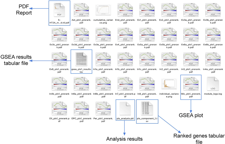
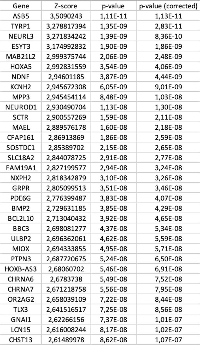
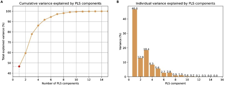
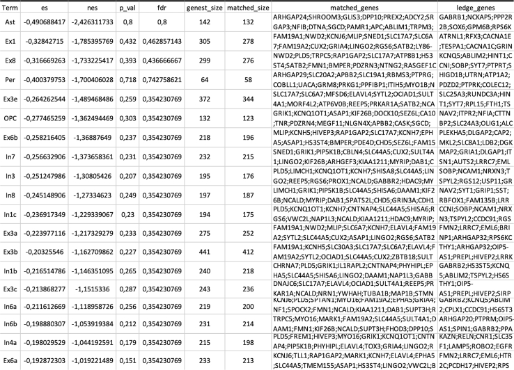
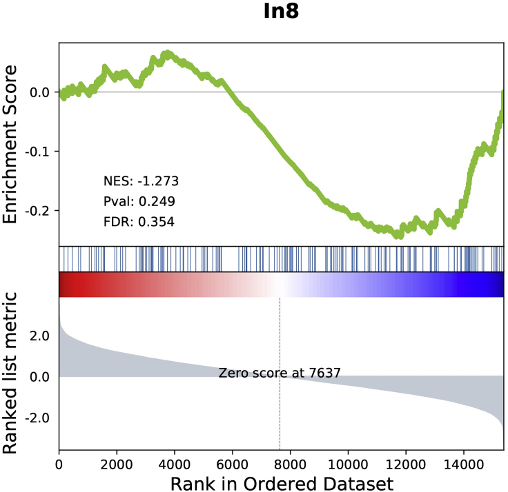
Once the analysis is completed, the toolbox creates a folder where the output files are stored (a typical example can be seen in Figure 1). The output files can be summarized as 1) a tabular file (i.e., pls_component_1.tsv Figure 1) with the results from the correlation analysis containing a list of ranked genes, the coefficient of correlation (z-score in the case of PLS analysis) and the uncorrected and FDR-corrected p values (Figure 3). Note that in the case of a PLS regression analysis, a different file is created for each of the PLS components. 2) A pkl file which contains null ranked list of genes to be used for a different enrichment analysis without having to re-run the entire analysis (i.e., pls_analysis.pkl, Figure 1); 3) A PDF file with a report of the analysis performed. In the case of the PLS analysis, the PDF will include plots of the individual and cumulative variance explained by the first 15 components, alongside with the R² and p value for each of the components used in the analysis (plots are also available in the output folder as graphics, i.e., cumulative_variance.png and individual_variance.png, Figure 2). 4) A tabular file with the GSEA results (gsea_pls1_results containing the term of the gene set, enrichment score (ES) and normalized enrichment score (NES) scores, uncorrected and FDR-corrected p-values, the size of the gene set term, the number of matched genes, the list of all matched genes and the list of edge genes (i.e., genes contributing the most to the enrichment signal) (Figure 4). 5) Enrichment plots for each individual term of the gene set used (all the files terminating in _prerank.pdf, Figure 5).

Figure 1.

Example of the structure of an output folder

The folder includes tabular files with the results of both the correlation analysis and the GSEA analysis, plots for the variance explained by each component in case of a PLS analysis and enrichment plots for the results from the GSEA analysis.

Figure 3.

Example of tabular file containing the results of gene ranking according to alignment with neuroimaging phenotype

The toolbox outputs a tabular file containing: i) gene ID, ranked according to strength of correlation; ii) z-score of gene weight in PLS component (or Spearman’s coefficient in case of mass-univariate correlation analysis); and iii) uncorrected and FDR corrected p values for each gene.

Figure 2.

Example of variance plots produced in case of a PLS analysis

(A) Cumulative variance explained by different PLS models with increasing number of components; (B) Individual variance explained by each of the first 15 components.

Figure 4.

Example of tabular file with the results from the GSEA analysis

The tabular file contains data about the enrichment score (ES), normalized enrichment score (NES), uncorrected p value (p_val), FDR corrected p value (fdr), number of genes in the gene set term (geneset_size), number of matched genes from the correlation results (matched_size), label of the matched genes (matched_genes) and ledge genes (ledge_genes) for each of the terms included in a certain gene set.

Figure 5.

Example of an enrichment plot from the GSEA analysis

The analysis produces a plot for each term of the gene set used. The top portion of the plot shows the running enrichment score (ES) for the gene set as the analysis walks down the ranked list. The score at the peak of the plot (the score furthest from 0.0) is the ES for the gene set. The middle portion of the plot shows where the members of the gene set appear in the ranked list of genes. The bottom portion of the plot shows the value of the ranking metric as you move down the list of ranked genes. The ranking metric measures a gene’s correlation with a phenotype. The value of the ranking metric goes from positive to negative as you move down the ranked list.

Limitations

One of the main limitations of the current implementation of the toolbox is the lack of flexibility regarding the parcellation used to map the neuroimaging and gene expression data. We setup the pipeline to use a standard and widely used parcellation (DK atlas), which provides a fairly coarse coverage of cortical and subcortical regions. However, we acknowledge that specific research questions might require other parcellations, which for now are not readily available to the user. In that case, the user can modify the original code to use other parcellations, but the gene expression matrix will have to be recalculated (e.g., by using abagen to remap gene expression to the parcellation chosen by the user). Moreover, all the analyses are based on data from the left hemisphere because the AHBA includes gene expression data of the right hemisphere for two donors only. While a general limitation of the field and not of this specific work, this aspect might raise issues when a certain neuroimaging phenotype is strongly lateralized to the right hemisphere.

Troubleshooting

Problem 1

The toolbox is installed but the scripts fail to launch from the command line (before you begin step 3).

Potential solution

Make sure that the virtual environment where you have installed the toolbox is activated. This can be seen in the terminal or by typing the command:

> which python

From the command line.

Problem 2

When running the command on an existing image I get an InvalidSizeError, e.g., imaging_transcriptomics.errors.InvalidSizeError: The provided file has a wrong shape. The file has shape: (182, 218, 182, 1). (step-by-step method details steps 2 or 3).

Potential solution

Reshape the image to match the correct input shape. In the case of 4D scans, select the image you want to analyze (i.e., a single volume or their average).

Problem 3

After the installation, the program fails to run because of a ModuleNotFoundError: No module named ‘sklearn.datasets.base’. (step-by-step method details step 2).

Potential solution

Re-install the sklearn python dependency by running the command:

> pip uninstall sklearn

Followed by the command:

> pip install sklearn

Problem 4

The installation of the ENIGMA Toolbox fails, raising some errors (before you begin step 4).

Potential solution

To overcome the errors in the ENIGMA Toolbox installation you need to manually install some python libraries which the toolbox depends on (e.g., Cython and NumPy). In addition you can look at specific versions of the packages listed on the environment file (i.e., https://github.com/molecular-neuroimaging/Imaging_Transcriptomics.git).

Resource availability

Lead contact

Further information and requests for resources and reagents should be directed to and will be fulfilled by the lead contact, Dr. Daniel Martins (daniel.martins@kcl.ac.uk).

Materials availability

This study did not generate new unique reagents.

Data and code availability

The Imaging Transcriptomics toolbox is available on GitHub at https://github.com/molecular-neuroimaging/Imaging_Transcriptomics (Giacomel et al., 2022). The data used as example in the protocol are available in the Neurobiology Research Unit’s website https://xtra.nru.dk/FS5ht-atlas/.

References

- Alexander-Bloch A., Giedd J.N., Bullmore E. Imaging structural co-variance between human brain regions. Nat. Rev. Neurosci. 2013;14:322–336. doi: 10.1038/nrn3465. [DOI] [PMC free article] [PubMed] [Google Scholar]
- Alexander-Bloch A., Raznahan A., Bullmore E., Giedd J. The convergence of maturational change and structural covariance in human cortical networks. J. Neurosci. 2013;33:2889–2899. doi: 10.1523/JNEUROSCI.3554-12.2013. [DOI] [PMC free article] [PubMed] [Google Scholar]
- Arnatkevičiūtė A., Fulcher B.D., Fornito A. A practical guide to linking brain-wide gene expression and neuroimaging data. Neuroimage. 2019;189:353–367. doi: 10.1016/j.neuroimage.2019.01.011. [DOI] [PubMed] [Google Scholar]
- Beliveau V., Ganz M., Feng L., Ozenne B., Højgaard L., Fisher P.M., Svarer C., Greve D.N., Knudsen G.M. A high-resolution in vivo atlas of the human brain’s serotonin system. J. Neurosci. 2017;37:120–128. doi: 10.1523/JNEUROSCI.2830-16.2016. [DOI] [PMC free article] [PubMed] [Google Scholar]
- Desikan R.S., Ségonne F., Fischl B., Quinn B.T., Dickerson B.C., Blacker D., Buckner R.L., Dale A.M., Maguire R.P., Hyman B.T., et al. An automated labeling system for subdividing the human cerebral cortex on MRI scans into gyral based regions of interest. Neuroimage. 2006;31:968–980. doi: 10.1016/j.neuroimage.2006.01.021. [DOI] [PubMed] [Google Scholar]
- Fang Z. GSEApy: Gene Set Enrichment Analysis in Python. Zenodo. 2020. [DOI] [PMC free article] [PubMed]
- Fulcher B.D., Arnatkeviciute A., Fornito A. Overcoming false-positive gene-category enrichment in the analysis of spatially resolved transcriptomic brain atlas data. Nat. Commun. 2021;12:2669. doi: 10.1038/s41467-021-22862-1. [DOI] [PMC free article] [PubMed] [Google Scholar]
- Giacomel A., Martins D., Frigo M., Turkheimer F., Williams S.C.R., Dipasquale O., Veronese M. The Imaging Transcriptomics Toolbox. Zenodo. 2022. [DOI] [PMC free article] [PubMed]
- Gorgolewski K.J., Fox A.S., Chang L., Schäfer A., Arélin K., Burmann I., Sacher J., Margulies D.S. Tight fitting genes: finding relations between statistical maps and gene expression patterns. 2014. [DOI]
- Hawrylycz M.J., Lein E.S., Guillozet-Bongaarts A.L., Shen E.H., Ng L., Miller J.A., van de Lagemaat L.N., Smith K.A., Ebbert A., Riley Z.L., et al. An anatomically comprehensive atlas of the adult human brain transcriptome. Nature. 2012;489:391–399. doi: 10.1038/nature11405. [DOI] [PMC free article] [PubMed] [Google Scholar]
- Jenkinson M., Beckmann C.F., Behrens T.E.J., Woolrich M.W., Smith S.M. FSL. Neuroimage. 2012;62:782–790. doi: 10.1016/j.neuroimage.2011.09.015. 20 YEARS of fMRI. [DOI] [PubMed] [Google Scholar]
- Lake B.B., Chen S., Sos B.C., Fan J., Kaeser G.E., Yung Y.C., Duong T.E., Gao D., Chun J., Kharchenko P.V., Zhang K. Integrative single-cell analysis of transcriptional and epigenetic states in the human adult brain. Nat. Biotechnol. 2018;36:70–80. doi: 10.1038/nbt.4038. [DOI] [PMC free article] [PubMed] [Google Scholar]
- Larivière S., Paquola C., Park B., Royer J., Wang Y., Benkarim O., Vos de Wael R., Valk S.L., Thomopoulos S.I., Kirschner M., et al. The ENIGMA toolbox: multiscale neural contextualization of multisite neuroimaging datasets. Nat. Methods. 2021;18:698–700. doi: 10.1038/s41592-021-01186-4. [DOI] [PMC free article] [PubMed] [Google Scholar]
- Markello R.D., Arnatkeviciute A., Poline J.-B., Fulcher B.D., Fornito A., Misic B. Standardizing workflows in imaging transcriptomics with the abagen toolbox. eLife. 2021;10:e72129. doi: 10.7554/eLife.72129. [DOI] [PMC free article] [PubMed] [Google Scholar]
- Markello R.D., Misic B. Comparing spatial null models for brain maps. Neuroimage. 2021;236:118052. doi: 10.1016/j.neuroimage.2021.118052. [DOI] [PubMed] [Google Scholar]
- Martins D., Giacomel A., Williams S., Turkheimer F., Dipasquale O., Veronese M. Imaging transcriptomics: convergent cellular, transcriptomic, and molecular neuroimaging signatures in the healthy adult human brain. Cell Rep. 2021;37:110173. doi: 10.1016/j.celrep.2021.110173. [DOI] [PubMed] [Google Scholar]
- MATLAB . The MathWorks Inc; Natick, Massachusetts: 2020. version 9.9.0 (R2020b) [Google Scholar]
- Morgan S.E., Seidlitz J., Whitaker K.J., Romero-Garcia R., Clifton N.E., Scarpazza C., van Amelsvoort T., Marcelis M., van Os J., Donohoe G., et al. Cortical patterning of abnormal morphometric similarity in psychosis is associated with brain expression of schizophrenia-related genes. Proc. Natl. Acad. Sci. U S A. 2019;116:9604–9609. doi: 10.1073/pnas.1820754116. [DOI] [PMC free article] [PubMed] [Google Scholar]
- Smith S.M., Jenkinson M., Woolrich M.W., Beckmann C.F., Behrens T.E.J., Johansen-Berg H., Bannister P.R., De Luca M., Drobnjak I., Flitney D.E., et al. Advances in functional and structural MR image analysis and implementation as FSL. Neuroimage. 2004;23:S208–S219. doi: 10.1016/j.neuroimage.2004.07.051. Mathematics Brain Imaging. [DOI] [PubMed] [Google Scholar]
- Váša F., Seidlitz J., Romero-Garcia R., Whitaker K.J., Rosenthal G., Vértes P.E., Shinn M., Alexander-Bloch A., Fonagy P., Dolan R.J., et al. Adolescent tuning of association cortex in human structural brain networks. Cereb. Cortex. 2018;28:281–294. doi: 10.1093/cercor/bhx249. [DOI] [PMC free article] [PubMed] [Google Scholar]
- Woolrich M.W., Jbabdi S., Patenaude B., Chappell M., Makni S., Behrens T., Beckmann C., Jenkinson M., Smith S.M. Bayesian analysis of neuroimaging data in FSL. Neuroimage. 2009;45:S173–S186. doi: 10.1016/j.neuroimage.2008.10.055. Mathematics Brain Imaging. [DOI] [PubMed] [Google Scholar]
Associated Data
This section collects any data citations, data availability statements, or supplementary materials included in this article.
Supplementary Materials
Data Availability Statement