Mathematical modeling and analysis of COVID-19: A study of new variant Omicron

Abstract

We construct a new mathematical model to better understand the novel coronavirus (omicron variant). We briefly present the modeling of COVID-19 with the omicron variant and present their mathematical results. We study that the Omicron model is locally asymptotically stable if the basic reproduction number ${\mathcal{R}}_0<1$, while for ${\mathcal{R}}_0\le 1$, the model at the disease-free equilibrium is globally asymptotically stable. We extend the model to the second-order differential equations to study the possible occurrence of the layers(waves). We then extend the model to a fractional stochastic version and studied its numerical results. The real data for the period ranging from November 1, 2021, to January 23, 2022, from South Africa are considered to obtain the realistic values of the model parameters. The basic reproduction number for the suggested data is found to be approximate ${\mathcal{R}}_0\approx 2.1107$ which is very close to the actual basic reproduction in South Africa. We perform the global sensitivity analysis using the PRCC method to investigate the most influential parameters that increase or decrease ${\mathcal{R}}_0$. We use the new numerical scheme recently reported for the solution of piecewise fractional differential equations to present the numerical simulation of the model. Some graphical results for the model with sensitive parameters are given which indicate that the infection in the population can be minimized by following the recommendations of the world health organizations (WHO), such as social distances, using facemasks, washing hands, avoiding gathering, etc.

1. Introduction

Omicron is a new variant of SARS-CoV-2 that causes the infection is known as the omicron virus. The omicron virus is the strain of COVID-19 which is observed in South Africa in the early days of November 2021. After the identification of the virus and its fast propagation, the virus hits other European countries with a large number of cases. The virus is less severe than the common COIVD-19 virus and its other variants such as the delta. It spread very easily than the other original virus such as COVID-19 and the delta strain. According the Center for Disease Control and Prevention (CDC) expects that anyone infected with the Omicron virus can infect other individuals either vaccinated or do not have any symptoms [1]. The common symptoms of the virus include, body ache, fatigue, runny nose, cough, congestion, etc. After the discovery of the virus in the country many countries of the world suspended their flights to South Africa in order to minimize the spread of the infection.

Coronavirus infections have been studied by many researchers and epidemiologists to curtail the disease and its further spread in the community. The researchers tried to develop the vaccine and vaccinized most of the individuals in order to better reduce the number of infected people and their future spread. Although, with the passage of time and the emergence of the new variants of COVID-19, the world still facing infections in many countries. Some mathematical models in integer and non-integer order to study the COVID-19 infections are discussed in this paper. For example, the early infection of COVID-19 in China through a very comprehensive mathematical model is discussed in [2]. The optimal control analysis for the elimination or control of the disease in Pakistan, by considering the real COVID-19 cases has been studied in [3]. The COVID-19 infection is transferrable to other healthy humans very fast, so the best and most effective way is to reduce the infection, is the isolation and quarantine, which is discussed through a mathematical modeling approach by the authors in [4]. The lockdown and its impact on disease control have been studied through a mathematical modeling approach in [5]. The authors considered an SEIR modeling approach using the real data from Italy and France and presented the disease control scenario for the epidemic [6]. Different reported cases and their modeling in Nigeria, with comparison, have been discussed in [7]. A fractional study on COVID-19 to address the isolation, quarantine, and environmental vital loads has been explored in [8]. A robust study on COVID-19 in a fractional environment is considered in [9]. The analysis of the COVID-19 infection modeling for the real cases in Saudi Arabia has been discussed in [10]. The intercity coupling network on COVID-19 infection is briefly studied in [11].

Fractional calculus that gaining attention from researchers around the world due to its many properties and its applications to physical and engineering problems. The heredity properties, the memory, and the crossover behavior can only be observed in a model with a fractional-order system. The fractional calculus with different fractional operators and their applications have been found, in integrodifferential equations [12], the development in the operators [13], [14], application to epidemiology [15], [16], [17], application to wave dynamics equations, [18], [19] etc. The COVID-19 model with time delay and stochastic differential equation is explored in [20]. A fractional model to study the COVID-19 infection with the singular and nonsingular kernel is studied in [21]. The Caputo fractional model for the study of COVID-19 infection is discussed in [22]. The authors in [23] formulated a mathematical model for addressing the COVID-19 infection using the role of the media campaign. Modeling and forecasting of the OCVID-19 in China are studied in [24]. The study of the unreported COVID-19 cases and its analysis is done in [25]. Using the concept of the new-generalized Caputo fractional derivative to obtain the numerical solution of the COVID-19 infection model is studied in [26]. The COVID-19 infection model using integer and non-integer orders has been examined in [27]. The SARS-CoV-2 model with time delay has been suggested in [28]. A fractional model to determine the peak of the infection in Brazil has been examined in [29]. The projection of the COVID-19 infection model with optimal control theory is discussed in [30]. The authors in [31] considered the infected cases in India and formulated a fractional model and obtained the results. A COVID-19 infection model with vaccination has been discussed in [32]. A fractional model suggested in [31] has been used to study the infected cases in Argentina. The authors proposed two vaccination models for COVID-19 disease in [33] and presented their numerical simulations. A fractional model for COVID-19 infection with optimal control analysis in [34] has been used to study the infection cases in Spain. The concept of the modified Euler method in [35] is used by the authors to study the fractional model for COVID-19 infection. The authors suggested the conditions for the global stability of the COVID-19 model in the disease-free case [36]. The COVID-19 infection via a nonlinear fractional model has been suggested in [37]. A mathematical model for COVID-19 is constructed in [38], to study the qualitative analysis of the model. The global dynamics of the COVID-19 model have been studied in [39].

The main goal of this work is to understand the dynamics of the new variant of COVID-19 known as the omicron through mathematical modeling. Using the omicron feature, we formulate the model and use the real data of the infected cases in South Africa for the period November 1, 2021, to January 2022, to parameterize the model parameters. The novel mathematical model for the omicron is considered further to obtain a second-order differential epidemic model to study the possible existence of the multi-layers/waves. Sensitivity analysis is performed to find out the most sensitives parameters that increase or decrease the basic reproduction number ${\mathcal{R}}_0$. We study further the model in the stochastic case and present the results. The rest of the results in the present study are organized is as follows: In Section 2, we study the formulation of the model based on the omicron variant. In Section 3, we study the model-related results, its local and global stability analysis, and the existence of the endemic equilibria. A model with a second-order time derivative is presented in Section 4. The model with a stochastic version is given in Section 5. Data analysis, global sensitivity analysis, and discussion of results are given in Section 6. Section 7 summarized the results.

2. Model framework

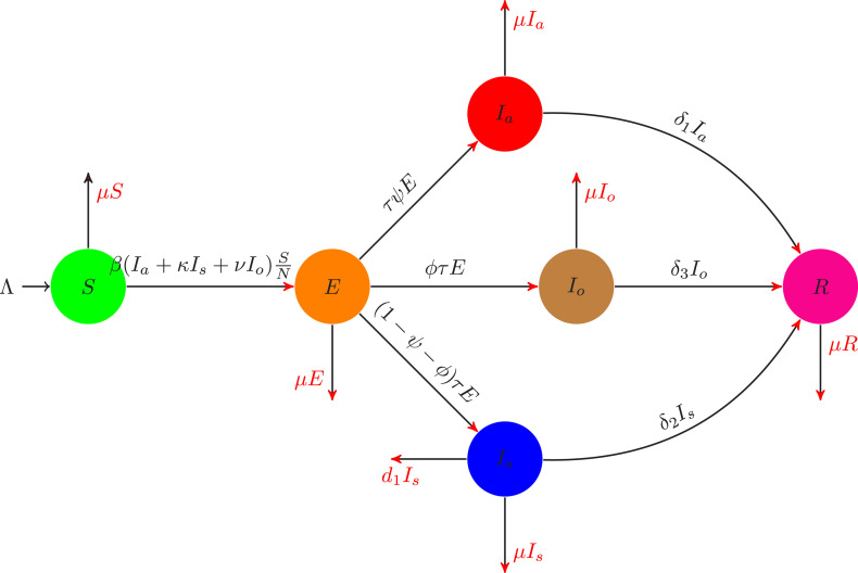
Due to the new variant of COVID-19 known as the Omicron virus, initially observed in South Africa, where the people faced once again many restrictions such as the SOPs to follow very strictly, maintain social distances, wearing face masks, etc. Many countries banned their flights to South Africa due to the new variant of COVID-19 which is spreading very fast. Keeping in view the Omicron variant, we considering formulating a very new mathematical model to understand the dynamics of the infection using the cases from South Africa. We consider the total population denoting it by $N\left(t\right)$, and dividing further into six different epidemiological classes: The individuals that attract the infection is given by $S\left(t\right)$ (which is not yet infectious), exposed individuals $E\left(t\right)$ (individuals after having contact with asymptomatic, symptomatic or individuals infected with omicron variant), asymptomatic individuals $I_a\left(t\right)$(individuals infected but they have no visible clinical symptoms), symptomatic individuals $I_s$ (individuals show clinical symptoms of COVID-19 infections), infected with omicron variant $I_o$ (individuals with clinical symptoms identified as omicron infected, an infected person with omicron infect other people whether it is vaccinated or do not have any disease symptoms), recovered individuals, $R\left(t\right)$ (individuals recovered from either asymptomatic, symptomatic or omicron variant). So, we have $N\left(t\right)=S\left(t\right)+E\left(t\right)+I_a\left(t\right)+I_s\left(t\right)+I_o\left(t\right)+R\left(t\right)$. Keeping in mind the discussion on the classes of the OCVID-19, we give the flow transmission from one compartment to another is given in Fig. 1, while the mathematical representation is given by the following evolutionary differential equations model:

$$\frac{dS\left(t\right)}{dt}=\Lambda -\frac{\beta (I_a+\kappa I_s+\nu I_o)}{N}S-\mu S,$$

$$\frac{dE\left(t\right)}{dt}=\frac{\beta (I_a+\kappa I_s+\nu I_o)}{N}S-(\tau +\mu )E,$$

$$\frac{d{I}_a\left(t\right)}{dt}=\tau \psi E-({\delta }_1+\mu )I_a,$$

$$\frac{d{I}_s\left(t\right)}{dt}=(1-\psi -\varphi )\tau E-({\delta }_2+\mu +d_1)I_s,$$

$$\frac{d{I}_o\left(t\right)}{dt}=\varphi \tau E-({\delta }_3+\mu )I_o,$$

$$\frac{dR\left(t\right)}{dt}={\delta }_1{I}_a+{\delta }_2{I}_s+{\delta }_3{I}_o-\mu R,$$ (1)

subject to the non-negative initial conditions. In the system (1), the parameter $\Lambda$ denote the birth rate of the susceptible population, while the people die naturally are shown by $\mu$. The healthy individuals infected after contacting the asymptomatic infected people by the rate $\beta$, while $\kappa$ and $\nu$ show the probability of infectiousness of symptomatic and with omicron variant respectively. The parameter $\tau$ shows the incubation period of the infected individuals. At a rate $\tau \psi$, the exposed individuals do not show clinical symptoms become to join the asymptomatic infected class while individuals show the clinical symptoms with common COVID-19 infection is given by the rate $(1-\psi -\varphi )\tau$ join the symptomatic infected class, where $\psi$ and $\varphi$ are the proportion that contribute the infection to asymptomatic class, and to the omicron variant infected class, while the rest are go to the symptomatic class. The recovery of the individuals of asymptomatic, symptomatic and omicron infected variant are given by the parameters ${\delta }_1$, ${\delta }_2$ and ${\delta }_3$ respectively. Individuals in the symptomatic class die to infection are shown by $d_1$. It should be noted that all new born are considered to be susceptible that can attract the infection.

Fig. 1.

Transmission diagram of the model (1).

3. Fundamental analysis of the model

Here, we study some of the important results related to the analysis of the model (1). We can get the total dynamics of the system (1) by adding all their equations, given by

$$\frac{dN}{dt}=\Lambda -\mu N-d_1{I}_s\le \Lambda -\mu N.$$ (2)

After solving the above Eq. (2), we get the following result,

$$N\left(t\right)=\frac{\Lambda }{\mu }+\left(N_0-\frac{\Lambda }{\mu }\right)e^{-\mu t}.$$ (3)

We can see that (3) tends to $\Lambda /\mu$ if $t\to \infty$. Also, it shows that the variables given in the model (1) are nonnegative for each value of $t\ge 0$. So, all the started solutions of the model (1) will remain positive for each $t\ge 0$. Therefore, the model given in (1) is mathematically well-posed and so its dynamical analysis can be studied in the following feasible region,

$$\Pi =\left\{\left(S,E,I_a,I_s,I_o,R\right)\in {\mathbb{R}}_{+}^6:S+E+I_a+I_s+I_o+R\le \frac{\Lambda }{\mu }\right\}.$$

Next, we are trying to show the solution positivity and boundedness of the model (1). The following results are presented:

3.1. Positivity and boundedness

We follow the results given in [40] to show the below result.

Theorem 1

The variables given in system (1) at $t=0$ ( $S\left(0\right)>0,E\left(0\right)>0,I_a\left(0\right)>0,I_s\left(0\right)>0,I_o>0,R\left(0\right)>0$ ) then the solution for $t>0$ of the variables involved in the system will be positive for every $t>0$ .

Proof

To show the result, let start from the equation of the model (1),

$$\frac{dS}{dt}=\Lambda -\lambda \left(t\right)S-dS\ge -(\lambda \left(t\right)+\mu )S,$$

where $\lambda \left(t\right)=\frac{\beta (I_a+\kappa I_s+\nu I_o)}{N}$. After taking the integration, we have the following result,

$$S\left(t\right)\ge S_{0}exp\left(-{\int }_0^t(\lambda \left(\tau \right)+\mu )\right)d\tau >0.$$

In the above inequality, $S_0$ denotes the initial population which is positive obviously, and thus, $S\left(t\right)$ is positive. We can easily follow the above mentioned procedure, to show the positivity of the rest of variables in the model (1), i.e., $E\left(t\right)>0$, $I_a\left(t\right)>0$, $I_s\left(t\right)>0$, $I_o\left(t\right)>0$ and $R\left(t\right)>0$. □

Further, to show the boundedness of the solution of the system (1), we discussed in the above theorem that the solution is positive and we can use Eq. (3) that for $t\to \infty$ is $\Lambda /\mu$, the solution is bounded.

3.2. Equilibrium points and its stability analysis

The disease-free equilibrium of the system (1) can be denoted by $E_0$ and is given by,

$$E_0=(S^0,0,0,0,0,0)=\left(\frac{\Lambda }{\mu },0,0,0,0,0\right).$$

Next, we use the next-generation approach for the computation of the basic reproduction number ${\mathcal{R}}_0$ The computation of the basic reproduction number ${\mathcal{R}}_0$ can be obtained through the next generation approach [41]. We have the following results after applying the method in [41],

$$F=\left(\begin{array}{cccc}\hfill 0\hfill & \hfill \beta \hfill & \hfill \beta \kappa \hfill & \hfill \beta \nu \hfill \\ \hfill 0\hfill & \hfill 0\hfill & \hfill 0\hfill & \hfill 0\hfill \\ \hfill 0\hfill & \hfill 0\hfill & \hfill 0\hfill & \hfill 0\hfill \\ \hfill 0\hfill & \hfill 0\hfill & \hfill 0\hfill & \hfill 0\hfill \end{array}\right),V=\left(\begin{array}{cccc}\hfill \mu +\tau \hfill & \hfill 0\hfill & \hfill 0\hfill & \hfill 0\hfill \\ \hfill -\tau \psi \hfill & \hfill \mu +{\delta }_1\hfill & \hfill 0\hfill & \hfill 0\hfill \\ \hfill \tau (\varphi +\psi -1)\hfill & \hfill 0\hfill & \hfill \mu +d_1+{\delta }_2\hfill & \hfill 0\hfill \\ \hfill -\tau \varphi \hfill & \hfill 0\hfill & \hfill 0\hfill & \hfill \mu +{\delta }_3\hfill \end{array}\right).$$

The spectral radius of $\varrho \left(F{V}^{-1}\right)$, gives the basic reproduction number is given by,

$${\mathcal{R}}_0=\underset{{\mathcal{R}}_1}{\underbrace{\frac{\beta \nu \tau \varphi }{\left({\delta }_3+\mu \right)(\mu +\tau )}}}+\underset{{\mathcal{R}}_2}{\underbrace{\frac{\beta \tau \psi }{\left({\delta }_1+\mu \right)(\mu +\tau )}}}+\underset{{\mathcal{R}}_3}{\underbrace{\frac{\beta \kappa \tau (1-\psi -\varphi )}{(\mu +\tau )\left(d_1+{\delta }_2+\mu \right)}}}.$$

Here ${\mathcal{R}}_1$ is an account for the cases generated through the contact of omicron infected with healthy people, ${\mathcal{R}}_2$ is responsible for the generation of secondary infection due to contact of healthy people with asymptomatic infected while ${\mathcal{R}}_3$ is an account for the cases due to symptomatic infection. The COVID-19 infection can be eliminated from the community if the numerical value of ${\mathcal{R}}_0<1$, otherwise the disease will spread in the community whenever ${\mathcal{R}}_0>1$. In the following section, we are establishing the stability results of the model (1) when ${\mathcal{R}}_0<1$ at the infection-free state.

Theorem 2

The COVID-19 infection model is locally asymptotically stable at infection-free equilibrium $E_0$ when ${\mathcal{R}}_0<1$ .

Proof

To get the stability results, we compute the Jacobian matrix of the model (1) at $E_0$, given by

$$J\left(E_0\right)=\left(\begin{array}{cccccc}\hfill -\mu \hfill & \hfill 0\hfill & \hfill -\beta \hfill & \hfill -\beta \kappa \hfill & \hfill -\beta \nu \hfill & \hfill 0\hfill \\ \hfill 0\hfill & \hfill -(\mu +\tau )\hfill & \hfill \beta \hfill & \hfill \beta \kappa \hfill & \hfill \beta \nu \hfill & \hfill 0\hfill \\ \hfill 0\hfill & \hfill \tau \psi \hfill & \hfill -(\mu +{\delta }_1)\hfill & \hfill 0\hfill & \hfill 0\hfill & \hfill 0\hfill \\ \hfill 0\hfill & \hfill \tau (1-\varphi -\psi )\hfill & \hfill 0\hfill & \hfill -(\mu +d_1+{\delta }_2)\hfill & \hfill 0\hfill & \hfill 0\hfill \\ \hfill 0\hfill & \hfill \tau \varphi \hfill & \hfill 0\hfill & \hfill 0\hfill & \hfill -(\mu +{\delta }_3)\hfill & \hfill 0\hfill \\ \hfill 0\hfill & \hfill 0\hfill & \hfill {\delta }_1\hfill & \hfill {\delta }_2\hfill & \hfill {\delta }_3\hfill & \hfill -\mu \hfill \end{array}\right)$$

The characteristics equation for the Jacobian matrix above is given by,

$${(\lambda +\mu )}^2[{\lambda }^4+a_1{\lambda }^3+a_2{\lambda }^2+a_3\lambda +a_4]=0,$$ (4)

where

$$a_1=d_1+{\delta }_1+{\delta }_2+{\delta }_3+4\mu +\tau ,$$

$$a_2=\left({\delta }_3+\mu \right)\left(d_1+{\delta }_2+\mu \right)+\left({\delta }_1+\mu \right)\left(d_1+{\delta }_2+{\delta }_3+2\mu \right)+(\mu +\tau )\left(d_1+{\delta }_2+\mu \right)(1-{\mathcal{R}}_3)+\left({\delta }_3+\mu \right)(\mu +\tau )(1-{\mathcal{R}}_1)+\left({\delta }_1+\mu \right)(\mu +\tau )(1-{\mathcal{R}}_2)$$

$$a_3=\left({\delta }_1+\mu \right)\left({\delta }_3+\mu \right)\left(d_1+{\delta }_2+\mu \right)+\left({\delta }_1+\mu \right)(\mu +\tau )\left(d_1+{\delta }_2+\mu \right)(1-{\mathcal{R}}_1-{\mathcal{R}}_2)+\left({\delta }_3+\mu \right)(\mu +\tau )(1-{\mathcal{R}}_2-{\mathcal{R}}_3)\left(d_1+{\delta }_2+\mu \right)+\left({\delta }_1+\mu \right)\left({\delta }_3+\mu \right)(\mu +\tau )(1-{\mathcal{R}}_1-{\mathcal{R}}_3),$$

$$a_4=\left({\delta }_1+\mu \right)\left({\delta }_3+\mu \right)(\mu +\tau )\left(d_1+{\delta }_2+\mu \right)(1-{\mathcal{R}}_0).$$ (5)

It can be seen from the above coefficients, that $a_1>0$, while $a_2$ and $a_3$ can be positive if the sub-reproduction number is less than unity and it is obviously less than ${\mathcal{R}}_0$ and hence $a_2$ and $a_3$ are positive. Further, the coefficient $a_4$ is positive whenever ${\mathcal{R}}_0<1$. So, it follows for the conditions of Routh–Hurwitz criteria, that $a_i>0$ for $i=1,2...,4$ are positive and further, it can be shown easily that $a_1{a}_2{a}_3>a_3^2+a_1^2{a}_4$. So, we conclude that all the eigenvalues computed for the Jacobian matrix at the equilibrium point $E_0$ have negative real parts and so, the model is locally asymptotically stable at the disease-free equilibrium whenever ${\mathcal{R}}_0<1$. □

Next, we study the global asymptotical stability of the model (1) at the disease-free case by follows the approach in [42]. Conditions to show the global asymptotical stability of the epidemic model, we need to construct a Lyapunov function that satisfies some conditions, (i) the constructed function should be positive definite, and (ii) the time derivative of the function along the solution of the model satisfy, $L^{\prime }\le -cL$, where $c$ is a positive constant.

Theorem 3

The infection model (1) at the equilibrium $E_0$ is globally asymptotically stable if ${\mathcal{R}}_0\le 1$ .

Proof

We construct for proof of the global stability, the following Lyapunov function,

$$L=f_{1}E+f_2{I}_a+f_3{I}_s+f_4{I}_o,$$ (6)

where $f_j>0$ for $j=1,2...,4$ are constants and can be determined later. Further, differentiating Eq. (6), and using the equations from the model (1), we have

$$\dot{L}=f_1\dot{E}+f_2\dot{I_a}+f_3\dot{I_s}+f_4\dot{I_o},=f_1[\frac{\beta (I_a+\kappa I_s+\nu I_o)}{N}S-(\tau +\mu )E]+f_2[\tau \psi E-({\delta }_1+\mu )I_a]+f_3[(1-\psi -\varphi )\tau E-({\delta }_2+\mu +d_1)I_s]+f_4[\varphi \tau E-({\delta }_3+\mu )I_o].$$ (7)

After some re-arrangements, Eq. (7) takes the following form:

$$\dot{L}=[f_1\beta -f_2({\delta }_1+\mu )]I_a+[f_1\beta \kappa -f_3({\delta }_2+\mu +d_1)]I_s+[f_1\beta \nu -f_4({\delta }_3+\mu )]I_o+[f_2\tau \psi +f_3(1-\psi -\varphi )\tau +f_4\varphi \tau -f_1(\tau +\mu )].$$ (8)

Let us choose the value for the constants: $f_1=({\delta }_1+\mu )$, $f_2=\beta$,

$f_3=\frac{\beta \kappa ({\delta }_1+\mu )}{({\delta }_2+\mu +d_1)}$, and $f_4=\frac{\beta \nu ({\delta }_1+\mu )}{({\delta }_3+\mu )}$, and using into the above Eq. (8), we get the following:

$$\dot{L}\le (\tau +\mu )({\delta }_1+\mu )\left(\frac{\beta \tau \psi }{(\tau +\mu )({\delta }_1+\mu )}+\frac{\beta \kappa \tau (1-\psi -\varphi )}{(\tau +\mu )({\delta }_2+\mu +d_1)}+\frac{\beta \nu \varphi \tau }{(\tau +\mu )({\delta }_3+\mu )}-1\right),=(\tau +\mu )({\delta }_1+\mu )({\mathcal{R}}_0-1)E.$$ (9)

Here, $\dot{L}\le 0$ whenever ${\mathcal{R}}_0\le 1$, and $\dot{L}=0$ if and only if $E=0$. Using $E=0$, in the equations of the model (1), we can get $(S,E,I_a,I_s,I_o,R)$ approaches to the infection free equilibrium $(S^0,0,0,0,0,0)$ for $t$ approaches to $\infty$. So, the largest invariant set will be the infection free equilibrium $E_0$. Thus, follows the results of LaSalles Invariance Principal that the system (1) is globally asymptotically stable in $\Pi$ if ${\mathcal{R}}_0\le 1$. □

3.3. Existence of endemic equilibria

To find the endemic equilibria of the model (1), we denote it by $Q_1$, and $Q_1=(S^{\ast },E^{\ast },I_a^{\ast },I_s^{\ast },I_o^{\ast },R^{\ast })$, so, we have

$$\left\{\begin{array}{c}{S}^{\ast }=\frac{\Lambda }{{\lambda }^{\ast }+\mu },\hfill \\ \hfill \\ E^{\ast }=\frac{{\lambda }^{\ast }{S}^{\ast }}{\mu +\tau },\hfill \\ \hfill \\ I_a^{\ast }=\frac{\tau \psi E^{\ast }}{{\delta }_1+\mu },\hfill \\ \hfill \\ I_s^{\ast }=\frac{\tau (1-\psi -\varphi )E^{\ast }}{d_1+{\delta }_2+\mu },\hfill \\ \hfill \\ I_o^{\ast }=\frac{\tau \varphi E^{\ast }}{{\delta }_3+\mu },\hfill \\ \hfill \\ R^{\ast }=\frac{{\delta }_1{I}_a^{\ast }+{\delta }_3{I}_o^{\ast }+{\delta }_2{I}_s^{\ast }}{\mu }.\hfill \end{array}\right)$$ (10)

Using the above into the expression given by

$${\lambda }^{\ast }=\frac{\beta (I_a^{\ast }+\kappa I_s^{\ast }+\nu I_o^{\ast })}{N^{\ast }},$$

we get the following,

$$g_1{\lambda }^{\ast }+g_2=0,$$

where

$$g_1=\left({\delta }_1+\mu \right)\left({\delta }_3+\mu \right)\left(d_1(\mu +\tau (\psi +\varphi ))+\left({\delta }_2+\mu \right)(\mu +\tau )\right),$$

$$g_2=\mu \left({\delta }_1+\mu \right)\left({\delta }_3+\mu \right)(\mu +\tau )\left(d_1+{\delta }_2+\mu \right)(1-{\mathcal{R}}_0).$$

Here, $g_1>0$ obviously, and we can have a positive $g_2$ if ${\mathcal{R}}_0<1$. To have a unique positive endemic equilibrium for the proposed model, we need to have ${\mathcal{R}}_0>1$. Thus, we have a unique positive endemic equilibrium when ${\mathcal{R}}_0>1$.

4. A model with second derivative

The second-order derivative is corresponds to the concavity or the curvature of the graph. The second-order derivative is used to determine the concave up and down of the function graph. A function whose second derivative is positive will be concave up, if negative it will be concave down, and if it is zero then it is possibly the inflection point. If the second derivative changes the sign from positive to negative then the function graph switch from concave up to concave down. This concept can also be used in epidemic models where there are many layers/waves for their infection cases. Usually, it is difficult to formulate a first-order model to give a better fit to the cases with many waves, so the second-order model with the above conditions may determine the concave up and down for an infection curve and leads to a better fit for the data to the proposed model. We give the following analysis to give details for our model, so, the following model is obtained after applying the second-order time derivative on the model (1), and we get the following updated model:

$$\frac{d^{2}S\left(t\right)}{d{t}^2}=-\frac{\beta [N(I_a\dot{S}+S\dot{I_a})-I_{a}S\dot{N}]}{N^2}-\frac{\beta \kappa [N(I_s\dot{S}+S\dot{I_s})-I_{s}S\dot{N}]}{N^2}-\frac{\beta \nu [N(I_o\dot{S}+S\dot{I_o})-I_{o}S\dot{N}]}{N^2}-\mu \dot{S},$$

$$\frac{d^{2}E\left(t\right)}{d{t}^2}=\frac{\beta [N(I_a\dot{S}+S\dot{I_a})-I_{a}S\dot{N}]}{N^2}+\frac{\beta \kappa [N(I_s\dot{S}+S\dot{I_s})-I_{s}S\dot{N}]}{N^2}+\frac{\beta \nu [N(I_o\dot{S}+S\dot{I_o})-I_{o}S\dot{N}]}{N^2}-(\tau +\mu )\dot{E},$$

$$\frac{d^2{I}_a\left(t\right)}{d{t}^2}=\tau \psi \dot{E}-({\delta }_1+\mu )\dot{I_a},$$

$$\frac{d^2{I}_s\left(t\right)}{d{t}^2}=(1-\psi -\varphi )\tau \dot{E}-({\delta }_2+\mu +d_1)\dot{I_s},$$

$$\frac{d^2{I}_o\left(t\right)}{d{t}^2}=\varphi \tau \dot{E}-({\delta }_3+\mu )\dot{I_o},$$

$$\frac{d^{2}R\left(t\right)}{d{t}^2}={\delta }_1\dot{I_a}+{\delta }_2\dot{I_s}+{\delta }_3\dot{I_o}-\mu \dot{R}.$$ (11)

The above model (11) will be used further to obtain, the strength number ${\mathcal{R}}_{st}$ for the model (11).

4.1. Strength number

In order to compute the strength number, we need to find the second derivative of the matrix $F$ as stated in above section of the computation of ${\mathcal{R}}_0$. We get

$$F_1=\left(\begin{array}{cccc}\hfill 0\hfill & \hfill -\frac{2\beta {\mu }^2}{{\Lambda }^2}\hfill & \hfill -\frac{2\beta \kappa {\mu }^2}{{\Lambda }^2}\hfill & \hfill -\frac{2\beta {\mu }^2\nu }{{\Lambda }^2}\hfill \\ \hfill 0\hfill & \hfill 0\hfill & \hfill 0\hfill & \hfill 0\hfill \\ \hfill 0\hfill & \hfill 0\hfill & \hfill 0\hfill & \hfill 0\hfill \\ \hfill 0\hfill & \hfill 0\hfill & \hfill 0\hfill & \hfill 0\hfill \end{array}\right),V=\left(\begin{array}{cccc}\hfill \mu +\tau \hfill & \hfill 0\hfill & \hfill 0\hfill & \hfill 0\hfill \\ \hfill -\tau \psi \hfill & \hfill \mu +{\delta }_1\hfill & \hfill 0\hfill & \hfill 0\hfill \\ \hfill \tau (\varphi +\psi -1)\hfill & \hfill 0\hfill & \hfill \mu +d_1+{\delta }_2\hfill & \hfill 0\hfill \\ \hfill -\tau \varphi \hfill & \hfill 0\hfill & \hfill 0\hfill & \hfill \mu +{\delta }_3\hfill \end{array}\right).$$

The spectral radius of $\rho \left(F_1{V}^{-1}\right)$, will give us the strength number denoted by ${\mathcal{R}}_{st}$,

$${\mathcal{R}}_{st}=-\frac{2\beta {\mu }^2\tau \left(\nu \varphi \left({\delta }_1+\mu \right)\left(d_1+{\delta }_2+\mu \right)+\psi \left({\delta }_3+\mu \right)\left(d_1+{\delta }_2+\mu \right)+\kappa \left({\delta }_1+\mu \right)\left({\delta }_3+\mu \right)(1-\psi -\varphi )\right)}{{\Lambda }^2\left({\delta }_1+\mu \right)\left({\delta }_3+\mu \right)(\mu +\tau )\left(d_1+{\delta }_2+\mu \right)}.$$

4.2. Analysis of the model (11)

Before, we study the model (11) further, we first update it further by considering the system (1) into (11), and get the model given by:

$$\frac{d^{2}E\left(t\right)}{d{t}^2}=\frac{\beta [N(I_a[\Lambda -\frac{\beta (I_a+\kappa I_s+\nu I_o)}{N}S-\mu S]+S[\tau \psi E-({\delta }_1+\mu )I_a])-I_{a}S[\Lambda -\mu N-d_1{I}_s]]}{N^2}+\frac{\beta \kappa [N(I_s[\Lambda -\frac{\beta (I_a+\kappa I_s+\nu I_o)}{N}S-\mu S]+S[(1-\psi -\varphi )\tau E-({\delta }_2+\mu +d_1)I_s])-I_{s}S[\Lambda -\mu N-d_1{I}_s]]}{N^2}+\frac{\beta \nu [N(I_o[\Lambda -\frac{\beta (I_a+\kappa I_s+\nu I_o)}{N}S-\mu S]+S[\varphi \tau E-({\delta }_3+\mu )I_o])-I_{o}S[\Lambda -\mu N-d_1{I}_s]]}{N^2}-(\tau +\mu )[\frac{\beta (I_a+\kappa I_s+\nu I_o)}{N}S-(\tau +\mu )E],$$

$$\frac{d^2{I}_a\left(t\right)}{d{t}^2}=\tau \psi \left[\frac{\beta (I_a+\kappa I_s+\nu I_o)}{N}S-(\tau +\mu )E\right]-({\delta }_1+\mu )[\tau \psi E-({\delta }_1+\mu )I_a],$$

$$\frac{d^2{I}_s\left(t\right)}{d{t}^2}=(1-\psi -\varphi )\tau \left[\frac{\beta (I_a+\kappa I_s+\nu I_o)}{N}S-(\tau +\mu )E\right]-({\delta }_2+\mu +d_1)\times \left[(1-\psi -\varphi )\tau E-({\delta }_2+\mu +d_1)I_s\right],$$

$$\frac{d^2{I}_o\left(t\right)}{d{t}^2}=\varphi \tau \left[\frac{\beta (I_a+\kappa I_s+\nu I_o)}{N}S-(\tau +\mu )E\right]-({\delta }_3+\mu )\left[\varphi \tau E-({\delta }_3+\mu )I_o\right].$$ (12)

Now considering the equilibrium points that is the disease-free and endemic case to show the possibility of concavity of the model (12). For this, we need to show that each equation of the model (12) which is in second-order that is the second-order time derivative greater than will show concave up, and if it is less than zero will determine to concave down otherwise for its value equal to zero is simply the inflection points. In order to analyze this, we first start from the disease-free case $E_0$ and using the system (12), we have: Using the disease-free equilibrium in the system (12), when the time rate of change is zero, we get all the equations of the model (12) gives zero, means simply the inflection points for the disease-free case, so we can say that there is no possibility of concave up or down at $E_0$. Further, to check the possibility of concave up, concave down, or simply the inflections points for endemic equilibrium $Q_1$, we check and give the explanations below:

$$\left\{\begin{array}{c}\frac{d^{2}E\left(t\right)}{d{t}^2}=0,\hfill \\ \hfill \\ \frac{d^2{I}_a\left(t\right)}{d{t}^2}=0,\hfill \\ \hfill \\ \frac{d^2{I}_s\left(t\right)}{d{t}^2}=0,\hfill \\ \hfill \\ \frac{d^2{I}_o\left(t\right)}{d{t}^2}=0.\hfill \end{array}\right)$$ (13)

One can see from (13) that all the second-order time derivatives for the computation of concavity using the second derivative test, we have only the case for the inflection or stationary points. So, it can be summarized that the model (12), at the disease-free and endemic equilibrium $E_0$ and $Q_1$ do not give the concave up and concave down but only simply the infection or the stationary points for the second-order model (12).

5. Stochastic fractional order model

This section presents, the mathematical modeling of the model (1) using the concept of Caputo orders piecewise fractional differential equations. The piecewise differential equations are used to fit the model with many waves, which is usually not possible for common models. The infection cases such as COVID-19 with many layers/waves are difficult to fit into the model, and hence the use of the piecewise differential equations may give a better fit to the data. The following model is presented:

$${}_0^C{D}_t^{q}S=\Lambda -\frac{\beta (I_a+\kappa I_s+\nu I_o)}{N}S-\mu S,$$

$${}_0^C{D}_t^{q}E=\frac{\beta (I_a+\kappa I_s+\nu I_o)}{N}S-(\tau +\mu )E,$$

$${}_0^C{D}_t^q{I}_a=\tau \psi E-({\delta }_1+\mu )I_a,$$

$${}_0^C{D}_t^q{I}_s=(1-\psi -\varphi )\tau E-({\delta }_2+\mu +d_1)I_s,$$

$${}_0^C{D}_t^q{I}_o=\varphi \tau E-({\delta }_3+\mu )I_o,$$

$${}_0^C{D}_t^{q}R={\delta }_1{I}_a+{\delta }_2{I}_s+{\delta }_3{I}_o-\mu R,$$ (14)

for the above model (14), we use $0\le t<T_1$. Next for the interval $T_1\le t<T_2$, we use the model:

$$\frac{dS\left(t\right)}{dt}=\Lambda -\frac{\beta (I_a+\kappa I_s+\nu I_o)}{N}S-\mu S,$$

$$\frac{dE\left(t\right)}{dt}=\frac{\beta (I_a+\kappa I_s+\nu I_o)}{N}S-(\tau +\mu )E,$$

$$\frac{d{I}_a\left(t\right)}{dt}=\tau \psi E-({\delta }_1+\mu )I_a,$$

$$\frac{d{I}_s\left(t\right)}{dt}=(1-\psi -\varphi )\tau E-({\delta }_2+\mu +d_1)I_s,$$

$$\frac{d{I}_o\left(t\right)}{dt}=\varphi \tau E-({\delta }_3+\mu )I_o,$$

$$\frac{dR\left(t\right)}{dt}={\delta }_1{I}_a+{\delta }_2{I}_s+{\delta }_3{I}_o-\mu R,$$ (15)

and finally for interval $T_2\le t\le T$, we have

$$dS=(\Lambda -\frac{\beta (I_a+\kappa I_s+\nu I_o)}{N}S-\mu S)dt+{\sigma }_{1}Sd{B}_1\left(t\right),$$

$$dE=(\frac{\beta (I_a+\kappa I_s+\nu I_o)}{N}S-(\tau +\mu )E)dt+{\sigma }_{2}Ed{B}_2\left(t\right),$$

$$I_a=(\tau \psi E-({\delta }_1+\mu )I_a)dt+{\sigma }_3{I}_{a}d{B}_3\left(t\right),$$

$$d{I}_s=((1-\psi -\varphi )\tau E-({\delta }_2+\mu +d_1)I_s)dt+{\sigma }_4{I}_{s}d{B}_4\left(t\right),$$

$$d{I}_o=(\varphi \tau E-({\delta }_3+\mu )I_o)dt+{\sigma }_5{I}_{o}d{B}_5\left(t\right),$$

$$dR=({\delta }_1{I}_a+{\delta }_2{I}_s+{\delta }_3{I}_o-\mu R)+{\sigma }_{6}Sd{B}_6\left(t\right).$$ (16)

Here ${\sigma }_k$ for $k=1,\dots ,6$ defines the constants that is the intensity of the stochastic environment and $B_k\left(t\right)$ for $k=1,\dots ,6$ is the standard Brownian motion. The Caputo derivative used in the above system (14), is given by the following:

$${}_0^C{D}_t^{q}G\left(t\right)=\frac{1}{\Gamma (1-q)}{\int }_0^t{(t-\tau )}^{-q}{G}^{\prime }\left(\tau \right)d\tau ,0<q\le 1.$$

Next, we consider the numerical solution to handle the above system is given by the following procedure:

$$\left\{\begin{array}{c}\hfill \frac{d{G}_m\left(t\right)}{dt}=g\left(t,G_m\right),\text{ if }0\le t\le T_1,\hfill \\ \hfill G_m\left(0\right)=G_{m,0},m=1,2,\dots ,n\hfill \\ \hfill \hfill \\ \hfill {}^C{D}_t^q{G}_m\left(t\right)=g\left(t,G_m\right),\text{ if }{T}_1\le t\le T_2\hfill \\ \hfill G_m\left(T_1\right)=G_{m,1},0<q\le 1,m=1,2,\dots ,n\hfill \\ \hfill \hfill \\ \hfill d{G}_m\left(t\right)=g\left(t,G_m\right)dt+{\sigma }_k{G}_{m}d{B}_k\left(t\right),\text{ if }{T}_2\le t\le T\hfill \\ \hfill G_m\left(T_2\right)=G_{m,2},m=1,2,\dots ,n.\hfill \end{array}\right)$$ (17)

The numerical scheme follows from [43], [44] and is given by: Dividing $[0,T]$ into three

$$0\le t_0\le t_1\le \cdots \le t_{m_1}$$

$$=T_1\le t_{m_1+1}\le t_{m_1+2}\le \cdots \le t_{m_2}=T_2\le t_{m_2+1}\le t_{m_2+2}\le \cdots \le t_{m_3}=T.$$

Then, we have the numerical scheme finally given by the following expression:

$$G_m^{m_1}=G_m\left(0\right)+\sum _{j_1=2}^{m_1}\left[\frac{23}{12}g\left(t_{j_1},G_{j_1}\right)-\frac{4}{3}g\left(t_{j_1-1},G_{j_1-1}\right)\right)\left(+\frac{5}{12}g\left(t_{j_1-2},G_{j_1-2}\right)\right]\Delta t,0\le t\le T_1$$

$$G_m^{m_2}=G_m\left(T_1\right)+\frac{{\left(\Delta t\right)}^q}{\Gamma (q+1)}\sum _{j_2=m_1+3}^{m_2}g\left(t_{j_2-2},G_{j_2-2}\right)\left[{\left(m_2-j_2+1\right)}^q-{\left(m_2-j_2\right)}^q\right]+\frac{{\left(\Delta t\right)}^q}{\Gamma (q+2)}\sum _{j_2=m_1+3}^{m_2}\left[g\left(t_{j_2-1},G_{j_2-1}\right)-g\left(t_{j_2-2},G_{j_2-2}\right)\right]\times \left\{\begin{array}{c}\hfill {\left(m_2-j_2+1\right)}^q\left(m_2-j_2+3+2q\right)\hfill \\ \hfill -{\left(m_2-j_2\right)}^q\left(m_2-j_2+3+3q\right)\hfill \end{array}\right\}+\frac{{\left(\Delta t\right)}^q}{2\Gamma (q+3)}\sum _{j_2=m_1+3}^{m_2}\left[g\left(t_{j_2},G_{j_2}\right)-2g\left(t_{j_2-1},G_{j_2-1}\right)\right)\left(+g\left(t_{j_2-2},G_{j_2-2}\right)\right]$$$$\left\{\begin{array}{c}\hfill {\left(m_2-j_2+1\right)}^q\left[\begin{array}{c}\hfill 2{\left(m_2-j_2\right)}^2+(3q+10)\left(m_2-j_2\right)\hfill \\ \hfill +2q^2+9q+12\hfill \end{array}\right]\hfill \\ \hfill -{\left(m_2-j_2\right)}^q\left[\begin{array}{c}\hfill \left(2{\left(m_2-j_2\right)}^2+(5q+10)\left(m_2-j_2\right)\right]\hfill \\ \hfill +6q^2+18q+12\hfill \end{array}\right]\hfill \\ \hfill T_1\le t\le T_2\hfill \end{array}\right\},$$ (18)

$$G_m^{m_3}=G_m\left(T_2\right)+\sum _{j_3=m_2+3}^{m_3}\left[\frac{23}{12}g\left(t_{j_3},G_{j_3}\right)-\frac{4}{3}g\left(t_{j_3-1},G_{j_3-1}\right)\right)\left(+\frac{5}{12}g\left(t_{j_3-2},G_{j_3-2}\right)\right]\Delta t+{\sigma }_k\sum _{j=m_2+3}^{m_3}{G}_m^{j_3}\left(B_k^{j_3}-B_k^{j_3-1}\right),T_2\le t\le T.$$

6. Data fitting and numerical results

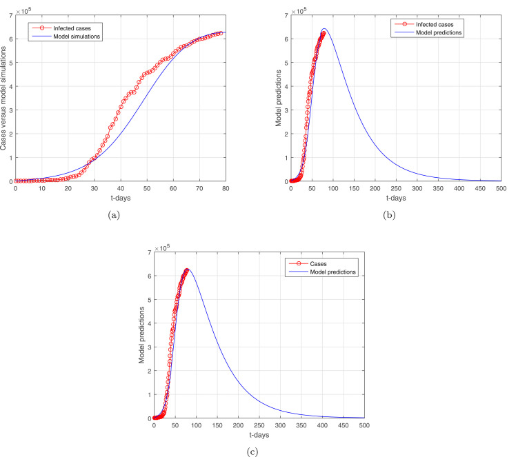
We consider the infected cases in South Africa reported from November 1, 2021, till January 23, 2022 [45]. The cases are considered daily wise with the unit per day. In the given model (1), there are 12 parameters, among these, the two parameters such as the natural birth rate, which is estimated, while the natural death rate is given by $(1/(64.38\times 365))$ [46], which is the average life expectancy of South African individuals at 2020–2021. The birth rate is computed through the formula, $N\left(0\right)=\Lambda /\mu$, where $N\left(0\right)$ is the total approximate population of South Africa in the year 2021. The South African population in 2021 is approximately considered to be $N\left(0\right)=60140000$. The healthy population in the disease absence is considered $S\left(0\right)=60069540$, and the other variables with the initial conditions subject to data fitting are $E\left(0\right)=62000$, $I_a\left(0\right)=8000$, $I_o\left(0\right)=100$, and $I_s\left(0\right)=360$ are the infected cases on November 1, 2021, and $R\left(0\right)=0$ (we assume that there is no recovery yet from the infection). We utilized the nonlinear least square method to fit the model to the suggested data with the period given above. The experiments were performed until the desired accurate fitting of the model is achieved. The nonlinear least square curve fitting method provides the realistic parameters values for the suggested data of the model (1) are obtained and have been shown in Table 1. The data fitting versus the model is shown in Fig. 2, where subgraphs (a–b) show respectively the data fitting versus the model and the predictions of the model for a large time level. The subgraph in Fig. 2 describes the simulation of the model for the stochastic case. The basic reproduction number ${\mathcal{R}}_0$ computed for the set of the parameters shown in Table 1 is obtained ${\mathcal{R}}_0\approx 2.1107$, which is considered to be very close to the actual one at South Africa.

Table 1.

Estimated parameters.

Symbol	Definition	Value/per day	Source
$\Lambda$	Birth rate	2553	Estimated
$\mu$	Natural death rate	$\frac{1}{64.38\times 365}$	Estimated
$\beta$	Contact rate	0.8999	Fitted
$\kappa$	Infectious of $I_s$	0.7800	Fitted
$\nu$	Infectious of $I_o$	0.4959	Fitted
$\tau$	Incubation period	0.8999	Fitted
$\psi$	The rate of flow to $I_a$	0.9566	Fitted
$\varphi$	The rate of flow to $I_o$	0.0101	Fitted
$d_1$	Disease death rate of asymptomatic people	0.0015	Fitted
${\delta }_1$	Recovery rate of $I_a$	0.8447	Fitted
${\delta }_2$	Recovery rate of $I_s$	0.0200	Fitted
${\delta }_3$	Recovery rate of $I_o$	0.6746	Fitted

Fig. 2.

Data versus model fitting: (a) data fitting versus model, (b) prediction of the model for large time level, (c) simulation of the model using stochastic model with ${\sigma }_1=0.0002$, ${\sigma }_2=0.002$, ${\sigma }_3=0.02$, ${\sigma }_4=0.02$, ${\sigma }_5=0.002$ and ${\sigma }_6=0.002$.

6.1. Global sensitivity analysis

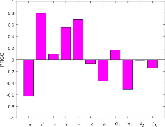
Global sensitivity analysis of the basic reproduction number ${\mathcal{R}}_0$ of the model (1) is considered. We use the combination of the Partial rank correlation coefficient (PRRC) and the Latin hypercube sampling (LHS) to have the global sensitivity results for the basic reproduction number ${\mathcal{R}}_0$. The PRCC is used to find out the most influential parameters involved in ${\mathcal{R}}_0$ that contribute to the variations of its value. In this analysis, we use the values of the parameters given in Table 1 and the corresponding sensitivity analysis is shown in Fig. 3. It can be observed from these sensitive parameters such as $\beta$, $\nu$, $\tau$, ${\delta }_1$, $\varphi$, $\mu$ etc, can increase or decrease the basic reproduction number ${\mathcal{R}}_0$. The contact rate of asymptomatic people, the contact rate $\nu$, the proportion of the exposed people who become asymptomatic, symptomatic, or omicron infected are the main drivers of the disease infection-causing. Similarly, the parameters ${\delta }_1$, $\mu$, and $\varphi$ also contribute to the variations in the basic reproduction number ${\mathcal{R}}_0$.

Fig. 3.

PRCC describes the impact of model parameters on ${\mathcal{R}}_0$ of the system (1).

6.2. Numerical results

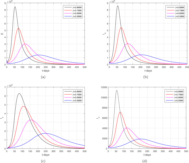
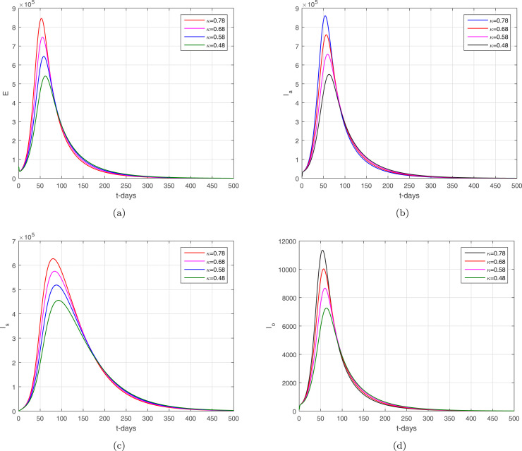
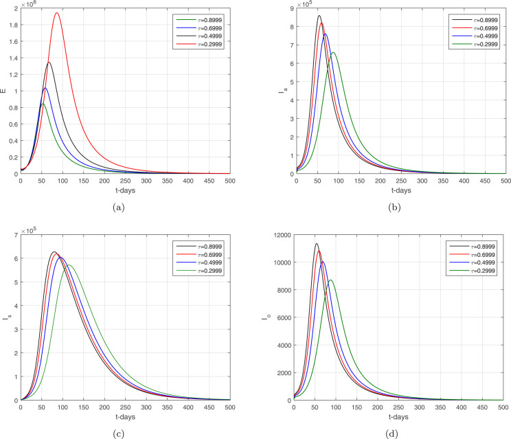
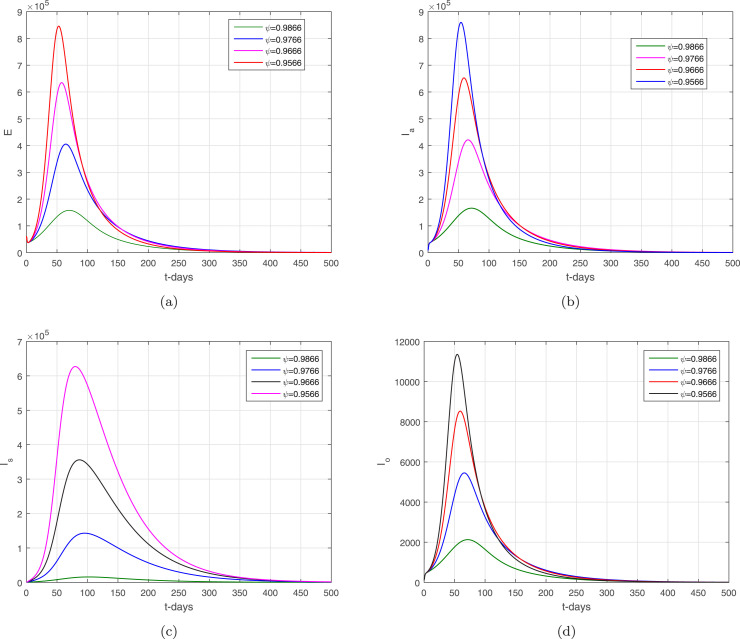
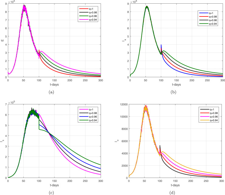
In the given section, we study the numerical simulation of the model given in (14)–(16). The parameters values considered in this simulation are given in Table 1, where we choose in this numerical simulation the time unit per day. The simulation results for the model (14)–(16) are shown in Fig. 4, Fig. 5, Fig. 6, Fig. 7, Fig. 8. Fig. 4 and their subgraphs describe the dynamics of the infected compartments with different values of the parameter $\beta$. Decreasing the contact, the number of infected individuals in each compartment is decreasing well. It shows that the contact among healthy individuals with asymptomatic, symptomatic, and individuals infected with omicron should be minimized in order to get the minimum infected cases in the community. The individuals infected with omicron are able to transmit the infection to other healthy individuals whether they are vaccinated or not possessing any disease symptoms. Due to the easy and high transfer rate of the virus from an infected person with omicron is considered more dangerous, and the possible prevention is to follow the recommendations of the WHO, which can curtail the disease infection cases. Fig. 5 shows the infected compartments and for various values of the parameter $\kappa$. With the decrease in the value of the $\kappa$, the number of infected people decreases over time. The individuals with clinical symptoms should be isolated, quarantined, or hospitalized, in order to prevent other healthy individuals from reducing the further spread of the disease. The most important is the infection generation of the individuals with no clinical symptoms and the fats spreading of the individuals infected with omicron should be considered with priority by reducing their contacts with other community individuals. The impact of the parameters $\tau$ and $\psi$ on the infected compartments of the model are shown in Fig. 6, Fig. 7. It can be observed from the results in Fig. 6, Fig. 7, that decreasing the values of the parameters a decrease occurred in the infected compartments of the individuals. Fig. 8 shows the dynamics of the infected compartments for different values of the fractional-order parameter.

Fig. 4.

The dynamics of the infected compartments of the model with $\beta =0.8999,0.7999,0.6999,0.5999$.

Fig. 5.

The dynamics of the infected compartments of the model with $\kappa =0.78,0.68,0.58,0.48$.

Fig. 6.

The dynamics of the infected compartments of the model with $\tau =0.8999,0.6999,0.6999,0.2999$.

Fig. 7.

The dynamics of the infected compartments of the model with $\psi =0.9866,0.9766,0.9666,0.9566$.

Fig. 8.

The dynamics of the infected compartments of the model with $q=1,0.98,0.96,0.94$.

7. Conclusion

A new mathematical model for the understanding of the new variant known as omicron has been presented. We formulated the model and presented in detail the biological process involved in the modeling of the omicron. We studied that the omicron model in the disease-free case is locally asymptotically stable if ${\mathcal{R}}_0<1$ and globally asymptotically stable if ${\mathcal{R}}_0\le 1$. The global stability of the omicron model implies, that the infection can only be controlled by reducing the basic reproduction number ${\mathcal{R}}_0$. The basic reproduction can be easily controlled to less than unity, if the social distancing, using of face masks, regularly washing the hands, avoiding gathering, staying at home, etc. The model positive endemic equilibria and their existence is shown, which shows that there are no possibilities of the backward bifurcation. Further, we constructed a model with a second-order derivative from the original model with time differentiation and then studied the possible occurrence of the layers. According to the given conditions from the second order model, there is no possibility of the occurrence of the possible waves in the present model. Furthermore, the omicron model is extended to the stochastic fractional case and presented a useful numerical scheme for its solution. The set of real values of the COVID-19 infection from Nov, 1, 2021–Jan, 23, 2022 has been considered to estimate the model parameters and obtained the basic reproduction number ${\mathcal{R}}_0\approx 2.1107$. The global sensitivity analysis is performed to obtain the most sensitive parameters that contribute to the variations in ${\mathcal{R}}_0$. The sensitivity analysis indicates, that contact among the healthy with asymptomatic, symptomatic, and individuals infected with omicron, can increase the infection further in the country. So, the recommendations of the WHO should be followed strictly, to reduce the spread of the omicron among other individuals. The novel numerical scheme is used to obtain the graphical result for the model using the values of the real parameters obtained from the data fitting. Various graphical illustrations for the model parameters and their impact on the disease eliminations were presented. From the suggested results, it can be seen that the disease can be eliminated following the recommendations of the World Health Ordination (WHO).

Declaration of Competing Interest

The authors declare that they have no known competing financial interests or personal relationships that could have appeared to influence the work reported in this paper.

References

- 1.Omicron Variant: What You Need to Know. https://www.cdc.gov/coronavirus/2019-ncov/variants/omicron-variant.html.
- 2.Khan Muhammad Altaf, Atangana Abdon. Modeling the dynamics of novel coronavirus (2019-nCov) with fractional derivative. Alexandria Eng. J. 2020;59(4):2379–2389. [Google Scholar]
- 3.Ullah Saif, Khan Muhammad Altaf. Modeling the impact of non-pharmaceutical interventions on the dynamics of novel coronavirus with optimal control analysis with a case study. Chaos Solitons Fractals. 2020;139 doi: 10.1016/j.chaos.2020.110075. [DOI] [PMC free article] [PubMed] [Google Scholar]
- 4.Khan Muhammad Altaf, Atangana Abdon, Alzahrani Ebraheem, et al. The dynamics of COVID-19 with quarantined and isolation. Adv. Difference Equ. 2020;2020(1):1–22. doi: 10.1186/s13662-020-02882-9. [DOI] [PMC free article] [PubMed] [Google Scholar]
- 5.Atangana Abdon. Modelling the spread of COVID-19 with new fractal-fractional operators: can the lockdown save mankind before vaccination? Chaos Solitons Fractals. 2020;136 doi: 10.1016/j.chaos.2020.109860. [DOI] [PMC free article] [PubMed] [Google Scholar]
- 6.López Leonardo, Rodo Xavier. A modified SEIR model to predict the COVID-19 outbreak in Spain and Italy: simulating control scenarios and multi-scale epidemics. Results Phys. 2021;21 doi: 10.1016/j.rinp.2020.103746. [DOI] [PMC free article] [PubMed] [Google Scholar]
- 7.Ayinde Kayode, Lukman Adewale F., Rauf Rauf I., Alabi Olusegun O., Okon Charles E., Ayinde Opeyemi E. Modeling Nigerian Covid-19 cases: A comparative analysis of models and estimators. Chaos Solitons Fractals. 2020;138 doi: 10.1016/j.chaos.2020.109911. [DOI] [PMC free article] [PubMed] [Google Scholar]
- 8.Oud Mohammed A. Aba, Ali Aatif, Alrabaiah Hussam, Ullah Saif, Khan Muhammad Altaf, Islam Saeed. A fractional order mathematical model for COVID-19 dynamics with quarantine, isolation, and environmental viral load. Adv. Difference Equ. 2021;2021(1):1–19. doi: 10.1186/s13662-021-03265-4. [DOI] [PMC free article] [PubMed] [Google Scholar]
- 9.Khan Muhammad Altaf, Ullah Saif, Kumar Sunil. A robust study on 2019-nCOV outbreaks through non-singular derivative. Eur. Phys. J. Plus. 2021;136(2):1–20. doi: 10.1140/epjp/s13360-021-01159-8. [DOI] [PMC free article] [PubMed] [Google Scholar]
- 10.Chu Yu-Ming, Ali Aatif, Khan Muhammad Altaf, Islam Saeed, Ullah Saif. Dynamics of fractional order COVID-19 model with a case study of Saudi Arabia. Results Phys. 2021;21 doi: 10.1016/j.rinp.2020.103787. [DOI] [PMC free article] [PubMed] [Google Scholar]
- 11.Lu Zhenzhen, Yu Yongguang, Chen YangQuan, Ren Guojian, Xu Conghui, Wang Shuhui, Yin Zhe. A fractional-order SEIHDR model for COVID-19 with inter-city networked coupling effects. Nonlinear Dynam. 2020;101(3):1717–1730. doi: 10.1007/s11071-020-05848-4. [DOI] [PMC free article] [PubMed] [Google Scholar]
- 12.Karthikeyan Kulandhivel, Karthikeyan Panjaiyan, Baskonus Haci Mehmet, Venkatachalam Kuppusamy, Chu Yu-Ming. Almost sectorial operators on -hilfer derivative fractional impulsive integro-differential equations. Math. Methods Appl. Sci. 2021 [Google Scholar]
- 13.Rashid Saima, Sultana Sobia, Karaca Yeliz, Khalid Aasma, Chu Yu-Ming. Some further extensions considering discrete proportional fractional operators. Fractals. 2022;30(01) [Google Scholar]
- 14.Rashid Saima, Abouelmagd Elbaz I., Sultana Sobia, Chu Yu-Ming. New developments in weighted n-fold type inequalities via discrete generalized-proportional fractional operators. Fractals. 2021 [Google Scholar]
- 15.He Zai-Yin, Abbes Abderrahmane, Jahanshahi Hadi, Alotaibi Naif D., Wang Ye. Fractional-order discrete-time SIR epidemic model with vaccination: Chaos and complexity. Mathematics. 2022;10(2):165. [Google Scholar]
- 16.Jin Fang, Qian Zi-Shan, Chu Yu-Ming, ur Rahman Mati. On nonlinear evolution model for drinking behavior under Caputo-Fabrizio derivative. J. Appl. Anal. Comput. 2022 [Google Scholar]
- 17.Gu Yu, Khan Muhammad Altaf, Hamed Y.S., Felemban Bassem F. A comprehensive mathematical model for SARS-CoV-2 in Caputo derivative. Fract. Fract. 2021;5(4):271. [Google Scholar]
- 18.Iqbal Md Ashik, Wang Ye, Miah Md Mamun, Osman Mohamed S. Study on date–Jimbo–Kashiwara–Miwa equation with conformable derivative dependent on time parameter to find the exact dynamic wave solutions. Fract. Fract. 2021;6(1):4. [Google Scholar]
- 19.Wang Fuzhang, Khan Muhammad Nawaz, Ahmad Imtiaz, Ahmad Hijaz, Abu-Zinadah Hanaa, Chu Yu-Ming. Numerical solution of traveling waves in chemical kinetics: time-fractional fishers equations. Fractals. 2022 [Google Scholar]
- 20.Rihan Fathalla A., Alsakaji Hebatallah J., Rajivganthi C. Stochastic SIRC epidemic model with time-delay for COVID-19. Adv. Difference Equ. 2020;2020(1):1–20. doi: 10.1186/s13662-020-02964-8. [DOI] [PMC free article] [PubMed] [Google Scholar]
- 21.Zhang Zizhen. A novel covid-19 mathematical model with fractional derivatives: Singular and nonsingular kernels. Chaos Solitons Fractals. 2020;139 doi: 10.1016/j.chaos.2020.110060. [DOI] [PMC free article] [PubMed] [Google Scholar]
- 22.Ali Aatif, Alshammari Fehaid Salem, Islam Saeed, Khan Muhammad Altaf, Ullah Saif. Modeling and analysis of the dynamics of novel coronavirus (COVID-19) with Caputo fractional derivative. Results Phys. 2021;20 doi: 10.1016/j.rinp.2020.103669. [DOI] [PMC free article] [PubMed] [Google Scholar]
- 23.Aldila Dipo. Analyzing the impact of the media campaign and rapid testing for COVID-19 as an optimal control problem in East Java, Indonesia. Chaos Solitons Fractals. 2020;141 doi: 10.1016/j.chaos.2020.110364. [DOI] [PMC free article] [PubMed] [Google Scholar]
- 24.Sun Deshun, Duan Li, Xiong Jianyi, Wang Daping. Modeling and forecasting the spread tendency of the COVID-19 in China. Adv. Difference Equ. 2020;2020(1):1–16. doi: 10.1186/s13662-020-02940-2. [DOI] [PMC free article] [PubMed] [Google Scholar]
- 25.Gao Wei, Veeresha P., Baskonus Haci Mehmet, Prakasha D.G., Kumar Pushpendra. A new study of unreported cases of 2019-nCOV epidemic outbreaks. Chaos Solitons Fractals. 2020;138 doi: 10.1016/j.chaos.2020.109929. [DOI] [PMC free article] [PubMed] [Google Scholar]
- 26.Erturk Vedat Suat, Kumar Pushpendra. Solution of a COVID-19 model via new generalized Caputo-type fractional derivatives. Chaos Solitons Fractals. 2020;139 doi: 10.1016/j.chaos.2020.110280. [DOI] [PMC free article] [PubMed] [Google Scholar]
- 27.Nabi Khondoker Nazmoon, Abboubakar Hamadjam, Kumar Pushpendra. Forecasting of COVID-19 pandemic: From integer derivatives to fractional derivatives. Chaos Solitons Fractals. 2020;141 doi: 10.1016/j.chaos.2020.110283. [DOI] [PMC free article] [PubMed] [Google Scholar]
- 28.Kumar Pushpendra, Suat Erturk Vedat. The analysis of a time delay fractional COVID-19 model via Caputo type fractional derivative. Math. Methods Appl. Sci. 2020 doi: 10.1002/mma.6935. [DOI] [PMC free article] [PubMed] [Google Scholar]
- 29.Kumar Pushpendra, Erturk Vedat Suat, Abboubakar Hamadjam, Nisar Kottakkaran Sooppy. Prediction studies of the epidemic peak of coronavirus disease in Brazil via new generalised Caputo type fractional derivatives. Alexandria Eng. J. 2021;60(3):3189–3204. [Google Scholar]
- 30.Nabi Khondoker Nazmoon, Kumar Pushpendra, Erturk Vedat Suat. Projections and fractional dynamics of COVID-19 with optimal control strategies. Chaos Solitons Fractals. 2021;145 doi: 10.1016/j.chaos.2021.110689. [DOI] [PMC free article] [PubMed] [Google Scholar]
- 31.Kumar Pushpendra, Suat Erturk Vedat. A case study of Covid-19 epidemic in India via new generalised Caputo type fractional derivatives. Math. Methods Appl. Sci. 2021 doi: 10.1002/mma.7284. [DOI] [PMC free article] [PubMed] [Google Scholar]
- 32.Kumar Pushpendra, Erturk Vedat Suat, Murillo-Arcila Marina. A new fractional mathematical modelling of COVID-19 with the availability of vaccine. Results Phys. 2021;24 doi: 10.1016/j.rinp.2021.104213. [DOI] [PMC free article] [PubMed] [Google Scholar]
- 33.Zeb Anwar, Kumar Pushpendra, Erturk Vedat Suat, Sitthiwirattham Thanin. A new study on two different vaccinated fractional-order COVID-19 models via numerical algorithms. J. King Saud Univ. Sci. 2022;34(4) doi: 10.1016/j.jksus.2022.101914. [DOI] [PMC free article] [PubMed] [Google Scholar]
- 34.Kumar Pushpendra, Erturk Vedat Suat, Nisar Kottakkaran Sooppy, Jamshed Wasim, Mohamed Mohamed S. Fractional dynamics of 2019-nCOV in Spain at different transmission rate with an idea of optimal control problem formulation. Alexandria Eng. J. 2022;61(3):2204–2219. [Google Scholar]
- 35.Nazir Ghazala, Zeb Anwar, Shah Kamal, Saeed Tareq, Khan Rahmat Ali, Khan Sheikh Irfan Ullah. Study of COVID-19 mathematical model of fractional order via modified Euler method. Alexandria Eng. J. 2021;60(6):5287–5296. [Google Scholar]
- 36.Zamir Muhammad, Shah Kamal, Nadeem Fawad, Bajuri Mohd Yazid, Ahmadian Ali, Salahshour Soheil, Ferrara Massimiliano. Threshold conditions for global stability of disease free state of COVID-19. Results Phys. 2021;21 doi: 10.1016/j.rinp.2020.103784. [DOI] [PMC free article] [PubMed] [Google Scholar]
- 37.Redhwan Saleh S., Abdo Mohammed S., Shah Kamal, Abdeljawad Thabet, Dawood S., Abdo Hakim A., Shaikh Sadikali L. Mathematical modeling for the outbreak of the coronavirus (COVID-19) under fractional nonlocal operator. Results Phys. 2020;19 doi: 10.1016/j.rinp.2020.103610. [DOI] [PMC free article] [PubMed] [Google Scholar]
- 38.Ali Zeeshan, Rabiei Faranak, Shah Kamal, Khodadadi Touraj. Qualitative analysis of fractal-fractional order COVID-19 mathematical model with case study of wuhan. Alexandria Eng. J. 2021;60(1):477–489. [Google Scholar]
- 39.ud Din Rahim, Seadawy Aly R., Shah Kamal, Ullah Aman, Baleanu Dumitru. Study of global dynamics of COVID-19 via a new mathematical model. Results Phys. 2020;19 doi: 10.1016/j.rinp.2020.103468. [DOI] [PMC free article] [PubMed] [Google Scholar]
- 40.Agusto F.B., Khan M.A. Optimal control strategies for dengue transmission in Pakistan. Math. Biosci. 2018;305:102–121. doi: 10.1016/j.mbs.2018.09.007. [DOI] [PubMed] [Google Scholar]
- 41.Van den Driessche Pauline, Watmough James. Reproduction numbers and sub-threshold endemic equilibria for compartmental models of disease transmission. Math. Biosci. 2002;180(1–2):29–48. doi: 10.1016/s0025-5564(02)00108-6. [DOI] [PubMed] [Google Scholar]
- 42.Korobeinikov Andrei, Wake Graeme C. Lyapunov functions and global stability for SIR, SIRS, and SIS epidemiological models. Appl. Math. Lett. 2002;15(8):955–960. [Google Scholar]
- 43.Atangana Abdon, Araz Seda Igret. Academic Press; 2021. New Numerical Scheme with Newton Polynomial: Theory, Methods, and Applications. [Google Scholar]
- 44.Atangana Abdon, Araz Seda İğret. Modeling third waves of Covid-19 spread with piecewise differential and integral operators: Turkey, Spain and Czechia. Results Phys. 2021;29 doi: 10.1016/j.rinp.2021.104694. [DOI] [PMC free article] [PubMed] [Google Scholar]
- 45.South Africa, Corona virus cases. https://www.worldometers.info/coronavirus/country/south-africa/.
- 46.South Africa - Life expectancy at birth. https://knoema.com/atlas/South-Africa/topics/Demographics/Age/Life-expectancy-at-birth.