

Abstract
Optimal profits for third-party logistics providers (3PLs) can be analyzed using the networks model to determine decision-making processes within transshipment and logistics, distribution networks, etc. Increasing academic attention is currently being focused upon fields examining 3PLs' operations within logistics networks. This paper studies cooperative game theory (CGT) of retailers-3PLs that make an alliance with each other with a specified demand function. The logistics network involves several suppliers and retailers-3PLs alliances, a distribution graph consisting of several nodes and arcs as well as multiple customers. Retailers-3PLs purchase the same goods from suppliers and sell to customers after shipping via the network; they also consider environmental issues to reduce pollutants and emissions fines. The proposed nonlinear programming (NLP) model aims to find the best flow and price of goods under cooperation conditions among retailers-3PLs by analyzing their risk levels. Controlling uncertainty in the models is accomplished by Mulvey's robust approach. In a general coalition, fair profit distribution methods are applied to share the profits among retailers-3PLs under different risk situations. We conduct a numerical analysis to present the application of our proposed model and find whether coalitions and cooperation between retailers-3PLs reduce costs and increase profits. Finally, we report the sensitivity analysis results regarding the penalties imposed for pollutant emissions, along with suggestions for future research. The results reveal that since their profit is greater in the coalition mode, they tend to cooperate with each other, whatever the amount of pollution fines be.
Keywords: Retailers-third party logistics providers (3PLs) alliances, Logistics networks, Cooperative game theory, Robust optimization (RO)
Introduction
The logistics industry has become increasingly focused on third-party logistics providers (3PLs) in recent years. Besides saving money, companies want to provide excellent services to their clients. In order to avoid logistical complications, they engage individual companies to handle all their logistics needs. There is a high demand for third-party services in the areas like transportation, warehouse management, consolidation of freight and handling, branding, marking and packing, stock control, recycling, order tracking as well as information technology for logistics (Rabinovich et al., 1999). Since the economic environment has become more competitive, companies now outsource their logistics to 3PLs (Hsiao et al., 2010; Li et al., 2012). According to a 2019 third-party logistics report (Third-Party Logistics Study, 2019), outsourcing accounts for 53% of shipper's shipping costs and 34% of warehouse operations costs. As a result, optimization in this area can create opportunities for companies to enhance customer experience, reduce asset costs, become more agile and concentrate on their core business.
In logistics networks and supply chains (SCs), the goal of all members is to maximize their profits. Therefore, it is necessary to consider an approach of cooperation or competition between the members. One approach aimed at maximizing the profits of network members is a game theory (GT) approach involving collaborative games. However, the collaborative approach method is often not sufficiently well-implemented in real-world scenarios. One reason is that the issue of profit-sharing has not been satisfactorily resolved. Profit-sharing is most commonly examined from a financial perspective and increasing an enterprise's profit by lowering its costs is considered a positive outcome (Zhuang et al., 2010). This paper examines a multilevel transportation network, determining the impacts of collaboration and competition between retailers-3PLs on their profit margins and the selling price of goods. The network contains several suppliers of goods, retailers-3PLs and customers. In previous papers, 3PLs have been considered as only performing logistics activities such as transportation and packaging, while the activities of buying and selling goods are carried out by other members (such as retailers) and operated independently. In this paper, it is assumed that the third-party logistics provider (3PL) and the retailer make an alliance with each other and form a company called retailer-3PL, which competes and cooperates with other companies while purchasing goods from suppliers, shipping and selling goods to customers; also, the approach of cooperative and competitive games between companies is examined. The emission rate is one of the factors affecting the costs of retailers-3PLs and their profits. Therefore, the issue is considered from an environmental point of view.
Employing 3PLs as logistical contractors can shift supply chain (SC) risks and uncertainties to 3PLs. However, research has shown that, under various circumstances, 3PLs's operating efficiency cannot always be assured (Hill, 2005; Slack et al., 2010). The inability to deliver during disruptions could lead to 3PL failure and exit from the market (Huo et al., 2008; Yeung et al., 2006). For example, according to a 2020 Covid-19 report (The Impact of COVID-19 on Logistics Study, 2020), logistics companies, such as transportation service companies, were directly affected by the COVID-19 pandemic and shipments of various goods in different modes of transport were reduced due to COVID-19-related restrictions. The impact and reduction of freight volume in maritime and air transport over the road were reported. Therefore, with the outbreak of coronavirus, the activities of 3PLs due to labor shortages (disease or health protocols), cargo restrictions for delivery, packaging, transportation and other logistics services were significantly impacted and reduced.
In general, logistics participants, including 3PLs, are exposed to two types of risk: (1) An inadequate supply–demand coordination risk and (2) Instability in the economy caused by civil unrest, labor conflicts or terrorist attacks (Klibi et al., 2010). This paper addresses the first risk type. In these circumstances, customer demand is highly unpredictable, uncertain and dynamic, having a variety of influences, including competition, consumer preferences, legislation and economic crises, among others. Typically, there are three approaches to dealing with the uncertainty of such problems, namely stochastic programming, fuzzy/possibilistic programming and robust optimization methods (Pishvaee et al., 2011). When the probability distributions of uncertain parameters are known via sufficient and reliable historical data, stochastic programming is used (Azaron et al., 2008). When uncertain parameters are expressed based on insufficient historical data and decision makers' (DMs) subjective opinions, probabilistic programming might be employed. The robust optimization method is applied when historical data about the uncertain parameters as well as infeasibility of the problem cannot be tolerated (Ben-Tal et al., 2009). In this method, uncertainty of parameters is assumed to be varied within the given set and the robust counterpart optimization model seeks for the solutions immunizing the problem for any potential realizations of uncertain parameters. It should be mentioned that there are major drawbacks in using the possibilistic and stochastic approach, such as the unavailability of historical data, subjective opinions of DMs and actual probability distributions for uncertain data. As a result, the best choice for dealing with parameter uncertainty in optimization issues is robust optimization models, which can create the optimum solution for every realization of the uncertainty in a given limited uncertainty set. Also, to the best of our knowledge, there is no research on applying the RO approach in the context of coopetition and cooperation among 3PLs-retailers in logistics networks.
In response to this uncertainty, a variety of vendors can form cooperative distribution alliance, which organizes and transports goods through 3PLs acting as a coordination center, according to the patterns of collaborative distribution centered on 3PLs enterprises. In this paper, in addition to distributing and transporting goods in the network, the purchase and sale of goods are done by companies consisting of 3PLs and retailers, which make an alliance with each other and form a new company. The best way to maximize profitability is to reduce the cost of purchasing and transporting goods, penalties for pollutant emissions and distributing subsequent profits. It can also reduce excess cross-transport to achieve welfare benefits, such as traffic reduction and protection of environment, by lowering pollutant emissions. The employed approach can be defined as: the cooperation and competition among companies with the aim of maximizing their profits under conditions of customer demand uncertainty. Following this, a few methods are applied for dividing the profits among companies. A major contribution of this paper is in exploring how competition and cooperation among retailers-3PLs affects profit, selling price of goods, flow of goods and emission of environmental pollutants; each of the participants has different risk-taking behaviors and may carry out purchasing, shipping and selling activities.
The purpose of this paper is to address the following questions:
What are the advantages of creating a collaborative environment between retailers-3PLs?
Which mechanism will allocate savings costs optimally between coalition members in the proposed models with different risk behaviors?
What is the effect of cooperation between retailers-3PLs on the pollutant emission rate and the resulting penalties?
The literature review of our research topic includes two parts: competitive and cooperative relationships within 3PLs SCs and RO of mathematical models related to 3PLs. In the first part, Mahmoudi et al. (2021) examined the issue of sustainable supply chain management in the presence of the government through implementing the transportation sector outsourcing strategy to a 3PL. The problem is studied according to different formats of competition and game theory is used to model the problem. Hosseini Motlagh et al. (2020) studied the issue of outsourcing the collection of defective drugs by a 3PL using the game theory approach. Initially, under the Stackelberg game model, a drug manufacturer outsourced drug recall management and the collection fee was paid to a 3PL company. Finally, a Nash bargaining model was proposed to divide the producer's profit and 3PL under the collection cost contract. With a GT approach, Mahmoudi et al. (2020) examined the stability of a SC, as well as its impact on the profits of other players in the SC by incorporating 3PLs. Chen et al. (2019) studied the pricing and order strategies of a third-party logistics provider and a predominant retailer. In order to calculate equilibrium orders and prices among SC members using GT, they used logistic service levels as an additional variable. Huang et al. (2019) investigated optimal SC strategies for a system with a supplier, a retailer and a 3PL. The optimal operational strategies were compared for both decentralized and centralized decision-making, and a SC coordination model was developed whereby the 3PL firm also provided financing services. Jamali and Rasti-Barzoki (2019) considered commodity prices, the greenness of the product of the first manufacturer and 3PLs factors, which included delivery time and carbon dioxide emissions in providing commodities to distant markets. Gong et al. (2018) conducted an analysis and survey of a 3PL's information technology (IT) investment. They also considered how IT investments affected SC profits and suggested some arrangements between manufacturers and 3PLs. Chen et al. (2017) presented a GT-based equilibrium model of retailer-led, closed-loop SCs using logistics outsourcing. Based on the analysis, they determined the optimal logistics decisions for each member of the SC. Giri and Sarker (2017) examined a SC that included a manufacturer, a 3PL and several retailers. According to their findings, the demand function was not deterministic. Yu and Xiao (2017) presented separate Stackelberg competition scenarios. Their SC included a producer, a retailer and a 3PL that produced fresh agricultural products. Two separate problem scenarios were considered and the effect of channel leadership was examined. Wu et al. (2015) presented a SC for fresh foods and assumed a logistics outsourcing channel for the manufacturer to use; in that channel, they considered a distributor. According to them, logistics services affected demand, both in terms of price and quantity, in their competitive SC setup. Yan et al. (2015) identified two alternative business models for recycled goods. According to the first model, goods were sold by manufacturers through retailers. Remanufactured goods were then collected by retailers for resale online and resold by those retailers. Products were sold to customers through retailers in the second model. For the collection and remanufacturing of goods, 3PLs were used. Zhang et al. (2015) investigated a competitive pricing situation for a 3PL that offered warehousing and transportation services. Jiang et al. (2014) explored decision-making and collaboration within a SC involving a manufacturer, two retailers and a 3PL that offered low-cost logistics services; GT methodology was used to investigate this model. Cai et al. (2013) investigated a food SC that involved a manufacturer, a 3PL and a distributor. They used a perishable-goods-like random demand feature. A deterioration of the quantity and quality of products was also presumed and SC participants were considered to be in competition. Huang et al. (2013) examined a SC with a retailer and a 3PL competing to collect the recycled materials. GT was applied to calculate prices for each member, based on the competition between the retailer and 3PL. When retailers are allowed to compete, Xiao-hua and Zhen-ning (2010) described how choosing a product for post-consumer recycling affected the price that consumers would pay for it.
The second part of the relevant literature is about the researches that focus on RO of mathematical models related to 3PLs. Abbasi et al. (2020) designed a multi-objective mixed integer nonlinear programming (MINLP) model for locating, designing and fortifying SC hubs and distribution centers that minimized the cost and time of the SC. An optimal solution was found by considering disrupting hubs and centers and utilizing plausible programming based on credibility. Ghafarimoghadam et al. (2019) created a robust model able to examine a 3PLs's logistical infrastructure and pricing strategy. They modeled uncertainty budget as a fuzzy number since the value of the parameter is epistemically uncertain. Ouhimmou et al. (2019) considered a distribution network design under uncertain demand conditions and discussed a RO approach. A decision was necessary regarding where to open warehouses and the size of the space to rent from 3PLs. For 3PLs, Daghigh et al. (2016) applied a two-objective model to develop logistics networks. Suyabatmaz et al. (2014) examined reverse logistics (RL), including the decision-making process applied for testing under uncertain supply conditions. To deal with uncertainties in stochastic RL network design, they used hybrid simulation-analytical modeling, employing mixed integer programming (MIP) models and simulation iteratively. Hendriks et al. (2012) considered a 3PL which had no control over supply and demand, and which was faced with the problem of delivering various goods from manufacturers to customers. A model-predictive control policy (MPC) created a practical network topology by optimizing decisions based on operational consideration made by the model. Jouzdani and Fathian (2012) proposed a robust mathematical model for a 3PL's route-planning problem. The issue was modeled as a robust multi-depot multiple traveling salesman problem (MmTSP), with the numerical results. In order to capture the complexities in RL, Xanthopoulos and Iakovou (2009) suggested a simulation-based solution approach. Ko and Evans (2007) proposed a network architecture based on 3PL. They used complex parameters to analyze logistics movements both forward and backward. An uncertainty component was incorporated into the model using modeling procedures, and the model was solved with a hybrid genetic algorithm. Zhang et al. (2007) developed a model for designing a remanufacturing logistics from a 3PL point of view using a RL method. By a fuzzy chance constrained programming model, a triangular fuzzy number was used to represent the backward demand parameters and transportation costs. Summaries of some of the noteworthy recent studies in the literature are shown in Tables 10 and 11 in Appendix.
Table 10.
Published papers applying GT to 3PL
| 3PL task | Decisions for 3PL | A game between a 3PL and SC members | Competition | Cooperation | GT approach | Environmental considerations | Sensitivity analysis | |||
|---|---|---|---|---|---|---|---|---|---|---|
| Transportation | Warehousing | Others | ||||||||
| Mahmoudi et al. (2021) | ✗ | ✗ | ✗ | Cost of transportation | One producer and one retailer | ✗ | ✓ | Nash | ✓ | ✓ |
| Hosseini-Motlagh et al.(2020) | ✗ | ✗ | Collector | Incentive offered to customers | One producer | ✓ | ✓ | Nash and Stackelberg | ✗ | ✓ |
| Mahmoudi et al. (2020) | ✓ | ✗ | ✗ | Cost of transportation | One manufacturer and multiple retailers | ✓ | ✗ | Stackelberg | ✓ | ✓ |
| Chen et al. (2019) | ✓ | ✗ | Packaging | Service price | One manufacturer and one retailer | ✓ | ✗ | Stackelberg | ✗ | ✓ |
| Huang et al. (2019) | ✓ | ✗ | ✗ | Transportation price | One supplier and one retailer | ✓ | ✗ | Stackelberg | ✗ | ✓ |
| Jamali and Rasti-Barzoki (2019) | ✓ | ✗ | ✗ | CO2 emission, delivery time | Two manufacturers and one retailer | ✓ | ✓ | Nash and Stackelberg | ✓ | ✓ |
| Gong et al. (2018) | ✗ | ✗ | IT service | On-time delivery rate | One manufacturer | ✗ | ✓ | Nash | ✗ | ✗ |
| Chen et al. (2017) | ✓ | ✓ | Recycling | Service price | One manufacturer and one retailer | ✓ | ✗ | Stackelberg | ✗ | ✗ |
| Giri and Sarker (2017) | ✓ | ✓ | ✗ | Logistic service cost | One manufacturer and multiple retailers | ✓ | ✗ | Stackelberg | ✗ | ✗ |
| Yu and Xiao (2017) | ✓ | ✗ | ✗ | Service level | One supplier and one retailer | ✗ | ✓ | Nash | ✗ | ✗ |
| Wu et al. (2015) | ✓ | ✗ | ✗ | Service price and quality | One distributer | ✓ | ✓ | Nash and Stackelberg | ✗ | ✗ |
| Yan et al. (2015) | ✗ | ✗ | Remanufacturing and recycling | Service price | One manufacturer and multiple retailers | ✓ | ✗ | Stackelberg | ✗ | ✗ |
| Zhang et al. (2015) | ✗ | ✓ | ✗ | Price based delivery date option | Multiple customers | ✓ | ✗ | Stackelberg | ✗ | ✓ |
| Jiang et al. (2014) | ✓ | ✗ | ✗ | Warehousing and transportation service price |
One manufacturer and one retailer |
✓ | ✗ | Stackelberg | ✗ | ✓ |
| Cai et al. (2013) | ✓ | ✗ | ✗ | Transportation price | One producer | ✓ | ✗ | Stackelberg | ✗ | ✗ |
| Huang et al. (2013) | ✗ | ✓ | ✗ | Service price | One manufacturer and one retailer | ✓ | ✗ | Stackelberg | ✗ | ✗ |
| Xiao-hua and Zhen-ning (2010) | ✗ | ✗ | Recycling | Service price | Two manufacturers and two retailers | ✓ | ✗ | Stackelberg | ✗ | ✓ |
| This study | ✓ | ✓ | purchasing and selling goods in alliances with retailers | Sale price and flow rate | Multiple retailers-3PLs | ✓ | ✓ | Nash | ✓ | ✓ |
Table 11.
RO of mathematical models related to 3PLs
| Papers | Mathematical programming | NLP | Type of logistic network | Source of uncertainty | Uncertainty modelling approach | ||
|---|---|---|---|---|---|---|---|
| MIP | MILP | MINLP | |||||
| Abbasi et al. (2020) | ✗ | ✗ | ✓ | ✗ | |||
| Ghafarimoghadam et al. (2019) | ✗ | ✓ | ✗ | ✗ | Forward reverse | Budget | Fuzzy RO approach |
| Ouhimmou et al. (2019) | ✓ | ✗ | ✗ | ✗ | Forward | Demand | Stochastic programming-Benders decomposition method |
| Daghigh et al. (2016) | ✗ | ✗ | ✓ | ✗ | Forward | Demand and cost | probabilistic programming |
| Suyabatmaz et al. (2014) | ✓ | ✗ | ✗ | ✗ | Reverse | Stochastic data | Two hybrid simulation-analytical modeling approaches |
| Hendriks et al. (2012) | ✗ | ✗ | ✗ | ✓ | Forward | Supply and demand | Stochastic programming-branch and bound method |
| Jouzdani and Fathian (2012) | ✓ | ✗ | ✗ | ✗ | Forward | Transportation cost | Robust convex programmingMulvey's approach |
| Xanthopoulos and Iakovou (2009) | ✗ | ✓ | ✗ | ✗ | Reverse | Inherent uncertainty and variability in product returns | A simulation-based solution approach |
| Ko and Evans (2007) | ✗ | ✗ | ✓ | ✗ | Forward reverse | The location of the client's manufacturing facilities, the client's markets, the volume of the products to be handled | Hybrid RO approach |
| Zhang et al. (2007) | ✗ | ✗ | ✓ | ✗ | Reverse | The collecting demand, transportation cost | Hybrid RO approach-fuzzy set theory |
| This study | ✗ | ✗ | ✗ | ✓ | Forward | Demand | Robust convex programming (Mulvey's approach) |
According to the above review and to the best of our knowledge, 3PLs play a large role in various industries as logistics companies. To the best of the author’s knowledge, no research is to found that considers interactions of 3PLs that make alliances with other members in the logistics networks. Thus, three primary contributions are provided in this study. First, this paper proposes a mechanism of competition and cooperation of retailers-3PLs alliances in the situations of uncertainty as a potential way to examine the mutual relationships of them and enabling retailres-3PLs to earn more profit. The main contributions of our work are that this paper considers the collaboration of retailers-3PLs in achieving the best flow, selling price of goods and reducing the emission of environmental pollutants and its penalties; different collaboration game mechanisms are employed to address the issue of aligning coalition payoffs with their risk behaviors. Second, we consider different levels of risk behaviors (i.e., low risk, medium risk and high risk) of retailers-3PLs. Also, RO approach is used to deal with the uncertainty of the parameters. Eventually, in previous papers, 3PLs as logistics companies, they provide logistics services such as delivery, packaging, transportation and warehousing; other members of the SC, such as retailers, buy and sell goods independently. In this paper, retailers and 3PLs make an alliance with each other, form a new company called retailer-3PL and work together to purchase, transport and sell goods.
The remainder of the paper is structured as follows. We present a definition of the problem, mathematical notations and assumptions for the model in Sect. 2. Specifically, robust mathematical models under non-cooperative and cooperative approaches are presented in Sect. 3. The results of the computations, as well as a discussion and description of their managerial implications, are provided in Sect. 4. Finally, the conclusions and some ideas for future research are presented in Sect. 5.
Problem description, mathematical notations and assumptions
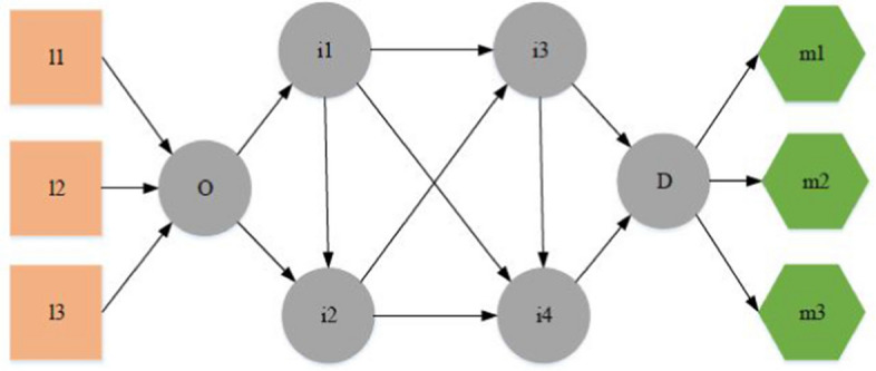
In this paper, a three-level logistics network is used as a platform. There are multiple suppliers with unlimited supply capacity, a distribution graph consisting of several nodes, origin node (node O) and destination node (node D), several customers with uncertain potential demand and several retailers-3PLs as companies (who purchase a type of product from suppliers according to their selling price and sell to customers after crossing the network). One of the decisions is to determine the optimal amount of shipping to reduce environmental pollution and its penalties, which could affect the profit of each retailers-3PLs as a function of customer demand, dependent on the selling price of goods. Then, the optimal shipping route must be determined, so that shipping costs in the network are reduced. There is also an assumption that the demand function is price-sensitive. Therefore, one more decision involves determining the optimal selling price of goods for each of the retailer-3PL, which affects the profit of each member. The SC is shown schematically in Fig. 1.
Fig. 1.

The schematic diagram of the network
As mentioned earlier, pricing decisions affect and maximize the profits of each retailer-3PL. The profit is the difference between revenue (the amount of sales multiplied by the price) and the costs of logistics. The SC budget contains the cost of purchasing the goods, the cost of handling between nodes and the penalty resulting from pollution emissions. Three-level nonlinear models are proposed to maximize profits for retailers-3PLs independently while forming coalitions among them in order to compete with each other and the other retailer-3PL.
In this section, the paper's mathematical notations are presented, both when retailers-3PLs operate independently and form coalitions, and when key assumptions are also examined. Table 1 shows the mathematical notations used when retailers-3PLs function independently.
Table 1.
Mathematical notations when retailers-3PLs operate independently
| Notation | Description |
|---|---|
| Index and sets | |
| Set of suppliers (l = 1,2,…,L) | |
| c | Set of retailers-3PLs(c = 1,2,…,C) |
| m | Set of customers (m = 1,2,…,M) |
| s | Set of scenarios sS |
| n | Coalition index |
| i,j,k | Index of nodes (initial or termination of arcs) (1, 2,…, N) |
| O | Origin node |
| D | Destination node |
| Input parameters | |
| A demand function scaling constant (> 0) in scenario s | |
| Demand function price elasticity for retailer-3PL c | |
| Demand function price elasticity for the competitors of retailer-3PL c | |
| Maximum fleet capacity (weight/volume) of retailer-3PL c | |
| Number of retailer-3PL c's fleet in scenario s | |
| Transportation (handling) cost per unit of good per unit of distance for retailer-3PL c | |
| Per unit purchase cost for supplier | |
| Distance between supplier and node j | |
| Distance between node i and node j | |
| Distance between node i and customer m | |
| Pollutant emission rate of transported per unit of good per unit of distance for retailer-3PL c | |
| Maximum budget of retailer-3PL c for transportation goods | |
| Penalty for emitting a polluted unit | |
| Probability of occurrence of scenario s | |
| Decision variables | |
|
Flow of good transported between supplier and node j by retailer-3PL c in scenario s |
|
| Flow of good transported between node i and node j by retailer-3PL c in scenario s | |
| Flow of good transported between node i and customer m by retailer-3PL c in scenario s | |
| Selling price of per unit good transported by retailer-3PL c to customer m | |
| Customer m's demand of retailer-3PL c in scenario s |
Table 2 provides the mathematical notations used while the retailers-3PLs form a coalition. In this paper, relates to the set of retailers-3PLs considered for the formation of a coalition.
Table 2.
Mathematical notations when retailers-3PLs form a coalition
| Notation | Description |
|---|---|
| Input parameters | |
| A demand function scaling constant(> 0) in coalition and c C in scenario s | |
| Demand function price elasticity for retailer-3PL c in coalition and c C | |
| Demand function price elasticity for the competitors of retailer-3PL c in coalition and c C | |
| Maximum fleet capacity (weight/volume) of retailer-3PL c | |
| Number of retailer-3PL c's fleet in coalition and c C in scenario s | |
| Transportation (handling) cost per unit of good per unit of distance for retailer-3PL c in coalition and c C | |
| Per unit purchase cost for supplier | |
| Distance between supplier and node j | |
| Distance between node i and node j | |
| Distance between node i and customer m | |
| Pollutant emission rate of transported per unit of good per unit of distance for retailer-3PL c in coalition and c C | |
| Maximum budget of retailer-3PL c for transportation goods in coalition and c C | |
| Penalty for emitting a polluted unit | |
| Probability of occurrence of scenario s | |
| Decision variables | |
| Flow of good transported between supplier and node j by retailer-3PL c in coalition and c C in scenario s | |
| Flow of good transported between node i and node j by retailer-3PL c in coalition and c C in scenario s | |
| Flow of good transported between node i and customer m by retailer-3PL c in coalition and c C in scenario s | |
| Selling price of per unit of good transported by retailer-3PL c to customer m in coalition | |
| Customer m's demand of retailer-3PL c in coalition and c C in scenario s | |
In modeling the described problem, the following assumptions are made:
All retailers-3PLs buy the same good from the same suppliers with unlimited supply capacity and with the same transport fleet; optimal routes are used for shipping across a network consisting of several nodes and arcs; goods are delivered to the customers and sold at the optimal price.
Players are a group of retailers-3PLs, all competing with each other and operating independently. Alternatively, a group of retailers-3PLs form a coalition and another retailer-3PL competes in the same network.
The sum of the goods that each retailer-3PL buys from suppliers is equal to the sum of the goods that it sells to its customers; the good is not lost in the network. It means that the flow into and out of each node is the same.
The risk sensitivity of the retailers-3PLs is assumed to assess the utility of the retailer-3PL (m) via revenue- (cost). In terms of flow and price, represents the attitude of the retailer-3PL. Moreover, when a set of retailers-3PLs form a coalition, it is assumed that the risk sensitivity of its members determines its risk attitude. It can thus be assumed that for coalition , a coalition's risk sensitivity is a linear combination of its members' risk sensitivity, i.e., , where and . This paper considers three cases of high risk averse coalition (HRAC), where , low risk averse coalition (LRAC), where , and moderate risk averse coalition (MRAC) where (Hafezalkotob & Makui, 2015).
- Following Azari Khojasteh et al. (2013), for each retailer-3PL, a demand function is used where is constant customer m's demand from retailer-3PL c in scenario s and is the retailer-3PL price sensitivity coefficient against customer demand. Also, is the competitive retailer-3PL price sensitivity coefficient against customer demand and . It is assumed that the demand function is linear and a function of the retailer-3PL selling price. The customer demand function is as follows:
1
Mathematical models
In this section, the stochastic model and the robust counterpart model of retailers-3PLs in two modes of independent activity and forming a coalition between them are presented.
Competitive and cooperative models
In competition and cooperation models, the profit of each retailer-3PL is calculated separately and each one has its profit function. The difference between the sales and costs of retailers-3PLs is used to measure the profit function. Costs include per unit of goods is transported at a specific cost per unit of distance, the cost of purchasing one unit of goods from the supplier and the cost of emitted pollution per unit of goods sent over distance.
In our proposed models, it is necessary for the total goods imported into a node to be equal to the total goods exported from that node. For each retailer-3PL, the total cost of shipping goods from suppliers to customers is less than or equal to the amount of shipping budget per retailer-3PL. There is an equal amount of shipping from suppliers and goods purchased from customers. Each customer's demand for goods is the total transported from the end node (node D) to that customer. The total goods carried by each retailer-3PL must be less than or equal to the capacity of the transport fleet. Based on the above, the stochastic model of retailers-3PLs operating in independent mode and in coalition mode can be stated as follows:
Mathematical model of retailers-3PLs in their independent activity
The NLP model of retailers-3PLs operating in the mode of independent activity, considering the defined notations in Table 1, is thus as follows:
| 2 |
Subject to:
| 3 |
| 4 |
| 5 |
| 6 |
| 7 |
| 8 |
| 9 |
| 10 |
| 11 |
| 12 |
The objective function (2) aims to maximize the profits derived from the difference in revenues and costs of each retailer-3PL (shipping cost, cost of purchasing goods and cost of emissions). The conservation of flow constraint (3) ensures the flow into a node must equal the flow out of every node; as a result, there is no loss of flow units. Constraint (4) is in charge of observing transport budget limitations for each of the retailers-3PLs. Constraint (5) guarantees that the total demand for goods for each retailer-3PL is equal to the total goods purchased from suppliers and that there is no shortage/surplus of goods. Constraint sets (6) and (7) mean that for each retailer-3PL, the total goods shipped on the network are equal to the total demand; hence, there is no loss of units while passing through the network. Constraint (8) assures that the total customer demand for retailer-3PL is equal to the sum of the goods that retailer-3PL provides to customers from the end node of the network and no commodity is lost along the way. Constraint (9) assures that the goods shipped to each customer are equal to that customer's demand and that each customer's demand is met without a shortage or surplus of goods. Constraint set (10) guarantees that the total goods loaded in the fleet of any retailer-3PL do not exceed the capacity of the fleet. Constraints (11) and (12) relate to the problem variables.
Mathematical model of retailers-3PLs in coalition mode
The NPL model of retailers-3PLs in the mode of coalition formation, considering the notations defined in Table 2, is thus as follows:
| 13 |
Subject to:
| 14 |
| 15 |
| 16 |
| 17 |
| 18 |
| 19 |
| 20 |
| 21 |
| 22 |
| 23 |
Objective function (13) and constraints (14)–(23) in the coalition mode are similar to the model in the retailers-3PLs independent activity mode. The exception to this is that, in the coalition mode, due to the cooperation of retailers-3PLs in the procurement, shipping and selling goods and meeting customer demand, the index is used in accordance with Table 2 for the relevant parameters and variables.
Proposed RO model
In our proposed model, there are some uncertain and scenario-based parameters such as potential customer demand, price sensitivity coefficients of the demand function, number of freight fleets, shipping cost, emission rate and a maximum budget of retailers-3PLs according to real-world conditions. Due to the lack of access to sufficient historical data and the mental opinions of decision makers to obtain the actual possible distribution, robust optimization approach is used to deal with uncertainty. Robust optimization is one of the most useful and popular methods in such situations for reducing the risk of uncertainty. According to Mulvey et al. (1995), RO should be used according to the problem conditions.
Mulvey's method was the first application of this principle of optimization. The results of this model are not significantly affected by scenario values and the obtained results are similar to the optimal values. Variables in this model have two types: control variables and design variables. It is not possible to modify design variables once the parameters have been set, but it is possible to change control variables. A constraint can be either structural or control, and the change in data will dictate the control constraint. In contrast, a structural constraint would correspond to a linear programming constraint.
When unknown parameters are present, the vector can represent control decision variables, as well as a decision variable vector, also called a design variable. When determining the optimal value of the design variables, uncertain parameters are also taken into account. Accordingly, the model has the following form:
| 24 |
Subject to:
| 25 |
| 26 |
| 27 |
Constraint (25) is a fundamental constraint not affected by variance in data. Constraint (26) is related to the control flow and the definitions of and are used. In each scenario, the probability of its occurrence is under the set of uncertain parameters within each scenario. An optimal and feasible solution is difficult to find in any case; a multi-criteria decision-making process must thus be used to strike a balance between the consistency of the solution and the consistency of the model. The feasibility of the solution is controlled by variable in the control constraint. According to Mulvey et al.’s (1995) approach, the RO optimization model is as follows:
| 28 |
Subject to:
| 29 |
| 30 |
| 31 |
An objective function's first expression indicates that the solution is stable and its second expression indicates that the model is established. The objective function of multiple scenarios is a random variable that has probability to take the value of . To achieve a robust optimum, the objective function expression can be transformed into predicted values and variances. The objective function can be maximized using one example. In addition, the objective function variance can be minimized in various circumstances, thus reducing the risk scale. The related formulation for this case is:
| 32 |
λ in Eq. (32) represents the level of risk in the model. As shown in Eq. (32), in the objective function, there is a quadratic argument. By contrast, Yu and Li (2000) used an absolute value, instead of the quadratic one:
| 33 |
However, the objective function remains nonlinear. In order to convert this function into a linear function, a non-negative variable and a constraint were added for each case by Yu and Li (2000). As a linear model, Eqs. (34)-(36) are used.
| 34 |
Subject to:
| 35 |
| 36 |
If is true, then, the minimization function is and the objective function is Also, if , then, the objective function must be stated as .
This approach leads to Eqs. (37)–(41) as the final linear model.
| 37 |
Subject to:
| 38 |
| 39 |
| 40 |
| 41 |
The following parameters and control variables are used to solve the problem in accordance with RO principles:
Addition of parameters to retailers-3PLs model in independent operation mode ():
Likelihood of scenario s occurring.
A value that is fixed.
Addition of parameters to retailers-3PLs model in coalition mode ():
Likelihood of scenario s occurring.
A value that is fixed.
Control variables:
Coefficient of linearization for scenario s for .
: Coefficient of linearization for scenario s for .
To consider the uncertainty of demand parameters in the objective function for retailers-3PLs, objective functions transformed the utilizing penalties based on profit per unit and . In order to consider the stability of response in the two independent modes of operation and coalition among retailers-3PLs, Sects. (3.2.1) and (3.2.2) of the robust counterpart model are formulated.
Robust counterpart model
The robust counterpart model in retailers-3PLs independent mode is as follows:
| 42 |
| 43 |
Subjected to:
| 44 |
| 45 |
| 46 |
| 47 |
| 48 |
| 49 |
| 50 |
| 51 |
| 52 |
| 53 |
| 54 |
Objective function (42), constraints (44)–(51) and constraints (53) and (54) are quite similar to objective function (2) and constraints (3)–(12) of the retailers-3PLs independent mode (Sect. 3.1.1). Regarding the added relation (43), there are two expressions for the objective function (43) within the optimization model: maximizing the mean of the profit functions of each scenario and maximizing their variance. A linearization constraint (52) of the objective function is also added to the model.
Robust counterpart model
The robust counterpart model in retailers-3PLs coalition mode is as follows:
| 56 |
Subject to:
| 57 |
| 58 |
| 59 |
| 60 |
| 61 |
| 62 |
| 63 |
| 64 |
| 65 |
| 66 |
| 67 |
Objective function (55), constraints (57)–(64) and constraints (66) and (67) are quite similar to the objective function (13) and constraints (14)–(23) of the retailers-3PLs coalition mode (Subsection 3.1.2). Regarding the added relation (56), specifically, in the first expression of objective function (56), everything is based on maximizing the mean of the profit function. The second function exists in order to maximize their variance. There is also a new constraint added to the model for linearizing objective function (65).
Computational results and discussion
Using a collaborative retailer-3PL framework, a numerical worked example is provided in this section.
Numerical study
In this section, a numerical example is provided to investigate the problem and further analyze the models and variables of retailers-3PLs. Figure 2 demonstrates the logistics network, in which retailers-3PLs operate. Considering the operation of retailers-3PLs under conditions of cooperation and independence, the risk sensitivity of retailers-3PLs are reported to be 0, 0.5 and 1, respectively. The benefits of independent activity against those of cooperation between retailers-3PLs are assessed using the Nash equilibrium. The numerical example is defined by considering three retailers-3PLs that buy the same goods with the same quality from three suppliers, transport them across the network and, finally, sell them to three customers while forming a coalition. Demand is determined by the amount of each customer's demand per order, as well as by the unit of weight of the order. The capacity of the retailers-3PLs fleet depends on the weight of the goods.
Fig. 2.
Multiple retailers-3PLs in a logistics network under uncertain demand
Two types of scenarios are considered in this paper. Two fundamental parameters of the demand equation are uncertain: the amount of fixed demand and amount of potential customer demand. In the first scenario, fixed demand is low, while the second scenario is associated with high fixed demand. In both scenarios, the probability of occurrence is 0.4 and 0.6. The values in Table 3 are assumed for the parameters in each scenario of this problem. All the parameter values are set according to the numerical examples in the literature and the problem conditions. To this end, two references including Jafarnejad et al. (2020) and Hafezalkotob and Makui (2015) have been considered. It should be noted the numbers are not exactly repeated, but the exact patterns are followed to find the most suitable values for these problems. Because the structures of the problems investigated in this study and those in the literature are significantly different, it is not possible to utilize the same values. The highest demand for a good is allocated to f, according to data from the literature review. Also, in each scenario, α and β (as the price sensitivity coefficients against demand) can have values between 0 and 1.
Table 3.
Values of parameters
| Parameters | Value of parameters |
|---|---|
| 4 × 10⁶, 4.4 × 10⁶, 4.6 × 10⁶ | |
| 3 × 10⁻⁶, 3.2 × 10⁻⁶, 3.4 × 10⁻⁶ | |
| 4 × 10⁻⁷, 4.5 × 10⁻⁷, 4.8 × 10⁻⁷ | |
| , , | |
| , , | |
| , , | |
| , | |
| , , , , , | |
| 1 × 10⁶, 1.2 × 10⁶, 1.3 × 10⁶ | |
|
|
|
|
|
|
| = 0, = 0.5, = 1 |
First, each of the retailer-3PL's cooperative robust problems will be solved individually as a non-cooperative case. Second, the issue of two retailers-3PLs coalitions will be resolved. Using this model, all three retailers-3PLs coalitions can be solved and the grand coalition will be reached. TU games should aim to maximize the profits of every coalition by maximizing the profits of each individual, according to the super-additive property, i.e., . The extra utility generated by coalition is calculated by summing the maximum profits of the coalition and its members, i.e., (Hafezalkotob & Makui, 2015). Coalition members should be individually evaluated for their additional utility. A more accurate indicator of a coalition's synergy is the following specification:
| 68 |
Based on the numerical example provided earlier, synergy () and EU () will be as follows (Table 4). Table 4 displays the problem's outputs for three risk scenarios: LRAC, MRAC and HRAC in the independent mode, as well as the creation of a coalition between retailers-3PLs. When the players work individually, the extra utilities and synergies are zero. Furthermore, the table shows that coalitions have nearly identical collaborative effects for their participants. In LRAC, retailer-3PL 1 joining with retailer-3PL 2 produces almost equal synergy (0.581) in comparison to retailer-3PL 3 (0.564). Therefore, retailers-3PLs may form coalitions together in any combination with similar synergies.
Table 4.
Calculating optimal profit, characteristic function and risk behavior of coalition members using various aggregation methods
| Coalition | ||||||||||
|---|---|---|---|---|---|---|---|---|---|---|
| LRAC | 6.222 | 15.222 | 2.50 × 10⁶ | 2.11 × 10⁶ | 2.30 × 10⁶ | 1.46 × 10⁷ | 1.46 × 10⁷ | 0 | 0 | |
| 5.817 | 14.817 | 2.36 × 10⁶ | 2.00 × 10⁶ | 1.91 × 10⁶ | 1.07 × 10⁷ | 1.07 × 10⁷ | 0 | 0 | ||
| 5.479 | 14.479 | 2.25 × 10⁶ | 1.91 × 10⁶ | 2.08 × 10⁶ | 1.18 × 10⁷ | 1.18 × 10⁷ | 0 | 0 | ||
| 12.442 | 30.442 | 3.95 × 10⁶ | 3.26 × 10⁶ | 3.61 × 10⁶ | 6.04 × 10⁷ | 6.04 × 10⁷ | 3.51 × 10⁷ | 0.581 | ||
| 12.406 | 30.406 | 3.95 × 10⁶ | 3.26 × 10⁶ | 3.60 × 10⁶ | 6.05 × 10⁷ | 6.05 × 10⁷ | 3.41 × 10⁷ | 0.564 | ||
| 12.003 | 30.003 | 3.73 × 10⁶ | 3.08 × 10⁶ | 3.40 × 10⁶ | 5.48 × 10⁷ | 5.48 × 10⁷ | 3.23 × 10⁷ | 0.590 | ||
| 18.102 | 45.102 | 4.84 × 10⁶ | 3.96 × 10⁶ | 4.40 × 10⁶ | 1.17 × 10⁷ | 1.17 × 10⁷ | 7.95 × 10⁷ | 0.682 | ||
| MRAC | 8.482 | 17.482 | 2.15 × 10⁶ | 1.76 × 10⁶ | 1.95 × 10⁶ | 7.41 × 10⁷ | 7.41 × 10⁷ | 0 | 0 | |
| 8.086 | 17.086 | 2.04 × 10⁶ | 1.67 × 10⁶ | 1.60 × 10⁶ | 5.75 × 10⁶ | 5.75 × 10⁷ | 0 | 0 | ||
| 7.75 | 16.75 | 1.95 × 10⁶ | 1.86 × 10⁶ | 1.77 × 10⁶ | 6.21 × 10⁷ | 6.21 × 10⁷ | 0 | 0 | ||
| 17.962 | 35.962 | 3.29 × 10⁶ | 2.60 × 10⁶ | 2.94 × 10⁶ | 3.59 × 10⁷ | 3.59 × 10⁷ | 2.28 × 10⁷ | 0.634 | ||
| 17.932 | 35.932 | 3.29 × 10⁶ | 2.60 × 10⁶ | 2.94 × 10⁶ | 3.58 × 10⁷ | 3.58 × 10⁷ | 2.22 × 10⁷ | 0.619 | ||
| 17.368 | 35.368 | 3.13 × 10⁶ | 2.48 × 10⁶ | 2.80 × 10⁶ | 3.21 × 10⁷ | 3.21 × 10⁷ | 2.02 × 10⁷ | 0.628 | ||
| 28.587 | 55.587 | 3.81 × 10⁶ | 2.93 × 10⁶ | 3.37 × 10⁶ | 6.94 × 10⁷ | 6.94 × 10⁷ | 5.00 × 10⁷ | 0.720 | ||
| HRAC | 8.482 | 17.482 | 2.15 × 10⁶ | 1.76 × 10⁶ | 1.95 × 10⁶ | 4.70 × 10⁷ | 4.70 × 10⁷ | 0 | 0 | |
| 8.087 | 17.087 | 2.00 × 10⁶ | 1.67 × 10⁶ | 1.86 × 10⁶ | 3.61 × 10⁷ | 3.61 × 10⁷ | 0 | 0 | ||
| 7.749 | 16.749 | 1.94 × 10⁶ | 1.60 × 10⁶ | 1.77 × 10⁶ | 3.89 × 10⁷ | 3.89 × 10⁷ | 0 | 0 | ||
| 17.962 | 35.962 | 3.29 × 10⁶ | 2.60 × 10⁶ | 2.94 × 10⁶ | 2.25 × 10⁷ | 2.25 × 10⁷ | 1.42 × 10⁷ | 0.631 | ||
| 17.933 | 35.933 | 3.29 × 10⁶ | 2.60 × 10⁶ | 2.94 × 10⁶ | 2.25 × 10⁷ | 2.25 × 10⁷ | 1.39 × 10⁷ | 0.617 | ||
| 17.361 | 35.361 | 3.13 × 10⁶ | 2.48 × 10⁶ | 2.80 × 10⁶ | 2.01 × 10⁷ | 2.01 × 10⁷ | 1.26 × 10⁷ | 0.627 | ||
| 28.677 | 55.667 | 3.81 × 10⁶ | 2.92 × 10⁶ | 3.37 × 10⁶ | 4.35 × 10⁷ | 4.35 × 10⁷ | 3.13 × 10⁷ | 0.720 |
The sale price variability through the coalitions' arcs is lower in HRAC and MRAC situations than in LRAC, as shown in Table 4. As the result of LRAC, the expected sale price of goods is higher. This means that the more conservatism of retailers-3PLs in the coalition, the lower the selling price of goods would be. With the increase in the risk sensitivity of retailers-3PLs and decrease in the selling price of goods, customer demand increases; therefore, the flow of goods in the network also increases. In Table 4, and show the amount of goods shipped by retailers-3PLs, which is equivalent to the total demand of 3 customers, in the two scenarios studied. The amount of good flow, or the total customer demand for each coalition, is higher in the second scenario than the amount of product flow in the first scenario due to the increase in consumer demand. Also, when retailers-3PLs operate independently, they make more profit in the LRAC and MRAC. On the other hand, when they form a coalition, they become more profitable in the LRAC, displaying optimal results with lower conservative risk behavior. The cooperative game theory (CGT) between retailers-3PLs is also additive in three different situations. Therefore, the extra utility and synergy increases proportionately with the coalition size until they become the most valuable extra utility. Benefits and synergies of larger coalitions also increase. It can thus be inferred that retailers-3PLs join coalitions at all three risk levels; when retailers-3PLs have moderate risk behavior, their additional income and synergy are higher and they have more tendency to forming a coalition.
Given that retailers-3PLs are looking to maximize profits, they will aim to reduce their total costs. To this end, retailers-3PLs are looking to find the optimal route to transport goods and select the appropriate supplier to reduce shipping costs, cost of pollutant emissions with regard to the shipping distance and cost of purchasing goods. In any coalition, retailers-3PLs will ship goods from node D to customers 1, 2 and 3, upon request. Table 5 shows the optimal route of retailers-3PLs in MRAC in the two studied scenarios.
Table 5.
Optimal transport route in MRAC
| Coalition | Scenario 1 | Scenario 2 |
|---|---|---|
| -O-1–3-5 | -O-1–2-3–4-5 | |
| -O-1–2-4–5 | -O-1–2-3–4-5 | |
| -O-2–4-5 | -O-1–4-5 | |
| -O-1–3-5 | -O-1–2-3–4-5 | |
| -O-2–4-5 | -O-1–2-3–4-5 | |
| -O-2–4-5 | -O-1–2-3–4-5 | |
| -O-1–3-5 | -O-1–2-3–4-5 |
In Table 6, PEC and PER show pollutant emission cost and pollutant emission rate in the independent mode and the cooperation of retailers-3PLs under moderate risk averse behavior in the two studied scenarios, respectively. In both scenarios, when retailers-3PLs work together and form a coalition, the costs of emissions (penalties) and emissions are less than the total cost and emission rates in their independent mode. Therefore, transporting goods in the form of a coalition and cooperation between retailers-3PLs reduces their costs, increases their profits and creates less pollution.
Table 6.
Pollutant emission cost and pollutant emission rate in MRAC
| Coalition | |||||
|---|---|---|---|---|---|
| MRAC | 3.6 × 10⁴ | 7.6 × 10⁴ | 1.8 × 10² | 3.8 × 10² | |
| 4.0 × 10⁴ | 8.4 × 10⁴ | 2.0 × 10² | 4.2 × 10² | ||
| 2.7 × 10⁶ | 8.8 × 10⁶ | 1.4 × 10⁴ | 4.4 × 10⁴ | ||
| 1.6 × 10⁵ | 4.3 × 10⁵ | 8.0 × 10² | 2.2 × 10³ | ||
| 1.7 × 10⁵ | 4.6 × 10⁵ | 8.5 × 10² | 2.3 × 10³ | ||
| 1.8 × 10⁵ | 4.9 × 10⁵ | 8.9 × 10² | 2.4 × 10³ | ||
| 4.1 × 10⁴ | 1.1 × 10⁶ | 2.0 × 10³ | 5.4 × 10³ |
Collaborative robust problem for retailers-3PLs
When the coalition benefits from retailers-3PLs cooperating, the utility should be shared among the participants. The main issue is how to distribute the coalition's benefits among various members. In response, various CGT methods have evolved optimal methods for distributing utility evenly (Mohammaditabar, 2015; Hajir et al., 2016; Tushar et al., 2018). Some of these methods will be briefly reviewed before adapting them to retailers-3PLs cooperative robustness. The proportion of utility distributed among coalitions is next calculated using well-known methods like the Shapley value, equal utility method (EUM) and the core center and least core.
A coalition made up of all players is defined as P = 1, 2, 3, …, N. If all players are participating in a coalition, v(P) refers to the available utility. Suppose that for each player, i = 1, 2, 3,…, N, is equal to the real numbers with . It is an imputation if vector = () satisfies the criterion of individual and group rationality, i.e., , and . As a result, the imputation set for a game will be Y = . The main CGT aim is to specify the form of imputation Y which offers a fair distribution of the overall gain. The concept of equal distribution has led to developing a number of different assignment methods, some of which are discussed here. More information can be found in Barron (2013) and Shapley (2010).
There are a series of allocations that ensure each alliance receives the least amount of incentives, which consists of:
| 69 |
According to Eq. (69), coalition excess is related to . If the core is not empty, the game is said to be stable. is defined for real number as:
| 70 |
The least core value of is . Solving the mathematical model below will also provide the least core value:
| 71 |
Subject to:
| 72 |
Shapley (1950) developed a method of assignment based on four efficiencies, symmetry, additive and dummy axioms. The Shapley value is a solution concept in cooperative game theory. It assigns a unique allocation (among the players) of a total surplus generated by the coalition of all players to each cooperative game. The Shapley value ensures each actor gains as much or more as they would have from acting independently. Because there is no other motivation for actors to collaborate, the value obtained is crucial. The Shapley value is one method of distributing the total gains among the players, given that they all cooperate. It is a "fair" distribution in the sense that it is the only distribution with certain desirable properties. An imputation denotes Shapley value if:
| 73 |
where N is the set of all coalitions that contain player P and represents the number of members in coalition C. gives the amount by which the cost saving of coalition increases when player P joins it. Therefore, represents the marginal cost saving of participate P with respect to coalition C. The formula of Shapley value denotes summation over all coalitions that contain player P (Zibaei et al., 2016).
Another allocation method is the EUM, which gives each utility an equal relative benefit (Audy et al., 2010). The maximum difference in usefulness between owners is reduced in this method. In order to calculate the EUM, one must solve the model:
| 74 |
Subject to:
| 75 |
| 76 |
| 77 |
Constraint (75) determines the difference between two players' relative profits. Additionally, Z is the greatest difference that should be minimized as a part of the objective function. Calculations for the least core and EUM are performed using Lingo 11 software. In MATLAB software, the TUGlab tool is used to calculate the rest of the results, which are presented in Table 7. In LRAC and with a lower conservative behavior, the profit allocated to each participant is higher; as shown in Table 4, when retailers-3PLs form a coalition, the profit in LRAC is higher than either MRAC or HRAC. Therefore, the profit allocated to each retailer-3PL is higher within the situations of lower risk sensitivity. Further, it appears that all methods (except least core) yield similar estimates.
Table 7.
Allocation of profits based on different allocation methods (values × 10–7)
| 3PL | Shapley | -Value | Core center | Least core | EUM | |
|---|---|---|---|---|---|---|
| LRAC | {1} | 4.19 | 4.20 | 4.22 | 6.18 | 4.60 |
| {2} | 3.71 | 3.71 | 3.70 | 1.07 | 3.36 | |
| (3) | 3.77 | 3.76 | 3.75 | 4.41 | 3.71 | |
| Stable | YES | YES | YES | YES | YES | |
| MRAC | {1} | 2.84 | 2.50 | 2.52 | 3.73 | 2.65 |
| {2} | 2.22 | 2.22 | 2.21 | 0.575 | 2.06 | |
| (3) | 2.24 | 2.23 | 2.21 | 2.64 | 2.22 | |
| Stable | YES | YES | YES | YES | YES | |
| HRAC | {1} | 1.56 | 1.57 | 2.52 | 2.34 | 1.68 |
| {2} | 1.39 | 1.39 | 2.21 | 0.3.61 | 1.29 | |
| (3) | 1.40 | 1.40 | 2.21 | 1.65 | 1.39 | |
| Stable | YES | YES | YES | YES | YES |
The core space under the grand coalition of retailers-3PLs is shown in Fig. 3. The core is the shaded zone. In this case, the game would have a convex shape since every edge of the imputation set is covered by the core. This means that retailers-3PLs will tend to form coalitions in all three risk-sensitive situations.
Fig. 3.

Core diagram and imputation
Coalition satisfaction is measured by as follows:
| 78 |
As the result of the S coalition's revenue, shows the difference between each player's revenue if they operated alone. When the criterion is higher, the players are more satisfied with their income. According to the corresponding formulas, Table 8 shows the level of satisfaction with each coalition.
Table 8.
Satisfaction of the coalition with different CGT methods
| Shapley | -value | Core center | Least core | EUM | |||||||
|---|---|---|---|---|---|---|---|---|---|---|---|
| Coalition surplus | Coalition satisfaction | Coalition surplus | Coalition satisfaction | Coalition surplus | Coalition satisfaction | Coalition surplus | Coalition satisfaction | Coalition surplus | Coalition satisfaction | ||
| LRAC | 2.73 × 10⁷ | 186.50 | 2.74 × 10⁷ | 187.34 | 2.76 × 10⁷ | 188.37 | 4.72 × 10⁷ | 322.82 | 3.13 × 10⁷ | 214.22 | |
| 2.64 × 10⁷ | 246.41 | 2.64 × 10⁷ | 246.21 | 2.63 × 10⁷ | 245.88 | 0 | 0 | 2.29 × 10⁷ | 214.22 | ||
| 2.59 × 10⁷ | 219.37 | 2.58 × 10⁷ | 218.51 | 2.57 × 10⁷ | 217.52 | 3.23 × 10⁷ | 273.97 | 2.53 × 10⁷ | 214.22 | ||
| 1.85 × 10⁷ | 30.68 | 1.86 × 10⁷ | 30.85 | 1.88 × 10⁷ | 31.04 | 1.21 × 10⁷ | 20.02 | 1.92 × 10⁷ | 31.69 | ||
| 1.90 × 10⁷ | 31.45 | 1.91 × 10⁷ | 31.48 | 1.91 × 10⁷ | 31.54 | 4.54 × 10⁷ | 75.02 | 2.25 × 10⁷ | 37.14 | ||
| 1.99 × 10⁷ | 36.36 | 1.98 × 10⁷ | 36.14 | 1.97 × 10⁷ | 35.86 | 0 | 0 | 1.59 × 10⁷ | 28.97 | ||
| Min | 1.85 × 10⁷ | 30.68 | 1.86 × 10⁷ | 30.85 | 1.88 × 10⁷ | 31.04 | 0 | 0 | 1.59 × 10⁷ | 28.97 | |
| Max | 2.73 × 10⁷ | 246.41 | 2.74 × 10⁷ | 246.21 | 2.76 × 10⁷ | 245.88 | 4.72 × 10⁷ | 322.82 | 3.13 × 10⁷ | 214.22 | |
| Sum | 1.37 × 10⁸ | 750.76 | 1.37 × 10⁸ | 750.53 | 1.37 × 10⁸ | 750.22 | 1.37 × 10⁸ | 691.83 | 1.37 × 10⁸ | 740.45 | |
| MRAC | 2.10 × 10⁷ | 283.84 | 1.76 × 10⁷ | 237.08 | 1.77 × 10⁷ | 239.50 | 2.98 × 10⁷ | 402.70 | 1.91 × 10⁷ | 258.27 | |
| 1.64 × 10⁷ | 285.86 | 1.64 × 10⁷ | 285.15 | 1.63 × 10⁷ | 284.04 | 1.10 × 10⁻¹ | 0 | 1.49 × 10⁷ | 258.27 | ||
| 1.61 × 10⁷ | 260.15 | 1.61 × 10⁷ | 258.65 | 1.59 × 10⁷ | 256.78 | 2.02 × 10⁷ | 325.18 | 1.60 × 10⁷ | 258.27 | ||
| 1.47 × 10⁷ | 40.98 | 1.12 × 10⁷ | 31.22 | 1.13 × 10⁷ | 31.54 | 7.08 × 10⁶ | 19.72 | 1.12 × 10⁷ | 31.29 | ||
| 1.50 × 10⁷ | 41.96 | 1.15 × 10⁷ | 32.02 | 1.15 × 10⁷ | 32.20 | 2.79 × 10⁷ | 77.86 | 1.30 × 10⁷ | 36.34 | ||
| 1.24 × 10⁷ | 38.60 | 1.23 × 10⁷ | 38.18 | 1.21 × 10⁷ | 37.62 | 2 | 0 | 1.07 × 10⁷ | 33.30 | ||
| Min | 1.24 × 10⁷ | 38.60 | 1.12 × 10⁷ | 31.22 | 1.13 × 10⁷ | 31.54 | 1.10 × 10⁻¹ | 0 | 1.07 × 10⁷ | 31.29 | |
| Max | 2.10 × 10⁷ | 285.86 | 1.76 × 10⁷ | 285.15 | 1.77 × 10⁷ | 284.04 | 2.98 × 10⁷ | 402.70 | 1.91 × 10⁷ | 258.27 | |
| Sum | 9.58 × 10⁷ | 951.40 | 8.50 × 10⁷ | 882.31 | 8.50 × 10⁷ | 881.68 | 8.50 × 10⁷ | 825.45 | 8.50 × 10⁷ | 875.72 | |
| HRAC | 1.09 × 10⁷ | 231.97 | 1.10 × 10⁷ | 233.71 | 2.05 × 10⁷ | 434.85 | 1.87 × 10⁷ | 397.43 | 1.21 × 10⁷ | 256.68 | |
| 1.03 × 10⁷ | 285.51 | 1.03 × 10⁷ | 284.82 | 1.85 × 10⁷ | 512.08 | 2.81 × 10⁻¹ | 0 | 9.26 × 10⁶ | 256.68 | ||
| 1.01 × 10⁷ | 259.82 | 1.01 × 10⁷ | 258.33 | 1.83 × 10⁷ | 468.63 | 1.26 × 10⁷ | 324.55 | 1.00 × 10⁷ | 256.68 | ||
| 6.99 × 10⁶ | 31.02 | 7.05 × 10⁶ | 31.27 | 2.47 × 10⁷ | 109.64 | 4.47 × 10⁶ | 19.83 | 7.11 × 10⁶ | 31.56 | ||
| 7.18 × 10⁶ | 31.96 | 7.20 × 10⁶ | 32.07 | 2.49 × 10⁷ | 110.69 | 1.75 × 10⁷ | 77.85 | 8.22 × 10⁶ | 36.59 | ||
| 7.78 × 10⁶ | 38.64 | 7.70 × 10⁶ | 38.23 | 2.41 × 10⁷ | 119.61 | 1 | 0 | 6.62 × 10⁶ | 32.87 | ||
| Min | 6.99 × 10⁶ | 31.02 | 7.05 × 10⁶ | 31.27 | 1.83 × 10⁷ | 109.64 | 2.81 × 10⁻¹ | 0 | 6.62 × 10⁶ | 31.56 | |
| Max | 1.09 × 10⁷ | 285.51 | 1.10 × 10⁷ | 284.82 | 2.49 × 10⁷ | 512.08 | 1.87 × 10⁷ | 397.43 | 1.21 × 10⁷ | 256.68 | |
| Sum | 5.33 × 10⁷ | 878.91 | 5.33 × 10⁷ | 878.42 | 1.31 × 10⁸ | 1755.49 | 5.33 × 10⁷ | 819.66 | 5.33 × 10⁷ | 871.05 | |
A coalition's minimum satisfaction level determines the minimum distance from the core. A coalition's responses in the core space will thus be evaluated according to this value. Simple calculations can also be performed using these values to determine the consistency of each answer. It can also be observed from Table 8 that, in the -value method, the utility is 7.05 × 10⁻⁶ at the lowest level of satisfaction. In all the methods and coalitions, retailers-3PLs are satisfied and dissatisfaction is not observed.
Various revenue allocation strategies are compared using the mean absolute deviation (MAD) index. A lower MAD value would indicate more efficient allocation of revenue, whereby the allocation of revenue to players would be similar. Equation (79) can be used to define this criterion:
| 79 |
indicates the amount of the discrepancies in each participant's earnings based on various methods. Table 9 shows the MRAC calculations for this index. The table's results demonstrate how different the outcomes of different methods are, as well as where the method results are similar. The Shapley, core center and EUM solutions all generate similar results. The results of various approaches to CGT vary widely; so, these features should be incorporated into player contracts.
Table 9.
Amount of absolute deviation
| MAD | Shapley | -value | Core center | Least core | EUM |
|---|---|---|---|---|---|
| Shapley | – | 2.87 | 0.22 | 1.76 | 0.22 |
| -value | – | – | 0.02 | 1.97 | 0.19 |
| Core center | – | – | – | 1.96 | 0.18 |
| Least core | – | – | – | – | 1.78 |
| EUM | – | – | – | – | – |
Figure 4 shows how pollution emission penalty sensitivity affects the Shapley values within a grand coalition under a robust cooperative model. We can see from the graph that as the penalty value rises, the Shapely value of retailers-3PLs decreases. As the fines for emissions increase and other parameters remain constant at the medium risk level, the cost of pollution increases. As a result, the profits of retailers-3PLs decrease. However, the profit of companies and their share in the Shapley value within the cooperative mode are higher than in the cases, in which they operate independently. Therefore, when the level of risk of companies is moderate, the increase of emission fines affects the profit of their coalition; in both cases, cooperative and independent, activity decreases.
Fig. 4.

Shapley values vs. pollution emission penalties sensitivity in MRAC
Managerial insights
The numerical example provides various management insights, which can be listed as follows:
Defining the price-sensitive demand function of a commodity can motivate retailers-3PLs to optimize their prices and compete with them by reducing costs.
The results reveal that retailers-3PLs are more profitable when they work together than when they operate independently. Therefore, it is suggested that companies use a cooperative approach and coalition profit-sharing to increase revenue.
Coalitions and cooperation between retailers-3PLs reduces costs and increases profits; in the situation of moderate risk sensitivity, they are more willing to form a coalition and their level of satisfaction with the coalition's overall utility is higher.
The results show that increasing emissions fines has a significant effect on coalition profits. Increasing pollution fines leads to lower profits for retailers-3PLs and their coalitions, both in coalition and independent modes. However, since their profit is greater in coalition mode, they tend to cooperate with each other, whatever the amount of pollution fines be. Also, cooperation between retailers-3PLs reduces emissions and the resulting fines relative to their independent mode of operation.
It is important to consider the risk of retailers-3PLs when forming coalitions and forming independent ventures. When retailers-3PLs operate independently, it is better to have low or moderate risk averse behaviors, and when forming a coalition, to be lower conservative and less risk-sensitive.
The alliance between retailers and 3PLs as well as the formation of independent companies makes all the activities of purchasing, selling and transporting goods carried out by one company and the profit earned is shared among the members.
Conclusions and future research
A new mathematical programming model was proposed in this paper, involving multiple retailers-3PLs and uncertain customer demand. A collaborative approach between retailers-3PLs was evaluated in order to raise the flow and price of goods by maximizing the expected value. As a result, the benefits of cooperation increased. From an environmental point of view, one of the important benefits was the reduction in pollutant emission rates and environmental costs, which affected the profit of each retailers-3PLs. Various collaborative game-based methods were analyzed through a numerical example, including the Shapley value, EUM, core center and least core methods. A risk structure for coalitions (namely LRAC, MRAC and HRAC) affected the ability of coalitions to perform additional functions and provide additive properties. The scale of the coalition increased the synergy of cooperation in all the three situations. There was a space core in all three risk modes. For the fair allocation of all cooperation rewards, members should prioritize realistic, rather than high-risk behaviors, since each member has an incentive to do so.
There are several possible directions of future research along the work presented here. First, in this paper, the constant demand parameter of customers is considered as an uncertain parameter. It is worth investigating the offered formulation in real cases where using parameters related to network uncertainty such as transportation cost, time and carrying capacity of routes. Second, this paper investigates the coopetition and cooperation among retailers-3PLs in the logistics network, while in the real logistics network, a legislator or manager often organizes the 3PLs to assure satisfying customers’ requirements. Thus, taking into account the role of a top level manager, considering other games such as Stackelberg between retailers-3PLs and the manager and investigating the impact of manager intervention policies on the retailers-3PLs's profits are interesting future research areas. Third, another interesting topic as the future works is to perform the proposed models for a real case study. A comprehensive and straightforward is presented that can be simply applied by someone to run to a real-world example. Fourth, in this paper, it is assumed it is impossible to stock goods within the network and that nothing would be lost during shipment. An interesting extension of the proposed models would be to accept these real-world conditions. Lastly, considering multi-period, multi-objective, multi-commodity and multi-vehicle is very interesting topics for extending this paper.
Acknowledgment
This paper has been accomplished on the basis of a Ph.D. dissertation by Nafiseh Fallahi supervised by Prof. Ashkan Hafezalkotob at Department of Industrial Engineering, South Tehran Branch, Islamic Azad University, Tehran, Iran. The authors would like to appreciate the reviewers and editor for their insightful comments.
Subscripts
- c
Set of retailers-3PLs (c = 1,2,…,C)
- D
Destination node
- i,j,k
Index of nodes (initial or termination of arcs) (1,2,…,N)
Set of suppliers (l = 1,2,…,L)
- m
Set of customers (m = 1,2,…,M)
- n
Coalition index
- O
Origin node
- s
Set of scenarios sS
Key variables
Customer m's demand of retailer-3PL c in scenario s
Customer m's demand of retailer-3PL c in coalition and c C in scenario s
Selling price of per unit good transported by retailer-3PL c to customer m
Selling price of per unit of good transported by retailer-3PL c to customer m in coalition cn
Flow of good transported between supplier and node j by retailer-3PL c in scenario s
Flow of good transported between supplier and node j by retailer-3PL c in coalition and c C in scenario s
Flow of good transported between node i and node j by retailer-3PL c in scenario s
Flow of good transported between node i and node j by retailer-3PL c in coalition and c C in scenario s
Flow of good transported between node i and customer m by retailer-3PL c in scenario s
Flow of good transported between node i and customer m by retailer-3PL c in coalition and c C in scenario s
Abbreviations
- CGT
Cooperative game theory
- DMs
Decision makers
- EU
Extra utility
- EUM
Equal utility method
- GT
Game theory
- HRAC
High risk averse coalition
- IT
Information technology
- Led
Leader
- LRAC
Low risk averse coalition
- MAD
Mean absolute deviation
- MINLP
Mixed integer nonlinear programming
- MIP
Mixed integer programming
- MmTSP
Multi-depot multiple traveling salesman problem
- MPC
Model-predictive control policy
- MRAC
Moderate risk averse coalition
- NLP
Nonlinear programming
- PEC
Pollutant emission cost
- PER
Pollutant emission rate
- 3PL
Third-party logistics provider
- 3PLs
Third-party logistics providers
- RL
Reverse logistics
- SC
Supply chain
- SCs
Supply chains
- TU
Transferable utility
Appendix
Footnotes
Publisher's Note
Springer Nature remains neutral with regard to jurisdictional claims in published maps and institutional affiliations.
Contributor Information
Nafiseh Fallahi, Email: Nafiseh_falahi1368@yahoo.com.
Ashkan Hafezalkotob, Email: a_hafez@azad.ac.ir, Email: ashkan.hafez@gmail.com.
Sadigh Raissi, Email: raissi@azad.ac.ir.
Vahidreza Ghezavati, Email: v_ghezavati@azad.ac.ir.
References
- Abbasi S, Sabouri A, Jabalameli M. Reliable supply chain network design for 3PL providers using consolidation hubs under disruption risks considering product perishability: An application to a pharmaceutical distribution network. International Journal of Computers & Industrial Engineering. 2020 doi: 10.1016/j.cie.2020.107019. [DOI] [Google Scholar]
- Audy JF, D'Amours S, Lehoux N, Rannqvist M. Coordination in collaborative logistics. International Workshop on Supply Chain Models for Shared Resource Management, Brussels. 2010;18:21–22. [Google Scholar]
- Azari Khojasteh M, Amin-Naseri M, Zegordi SH. Competitive pricing in a supply chain using a game theoretic approach. Iranian Journal of Operations Research. 2013;4(2):161–174. [Google Scholar]
- Azaron A, Brown KN, Tarim SA, Modarres M. A multi-objective stochastic programming approach for supply chain design considering risk. International Journal of Production Economics. 2008;116:129–138. doi: 10.1016/j.ijpe.2008.08.002. [DOI] [Google Scholar]
- Barron E. Game theory: An introduction. Wiley; 2013. [Google Scholar]
- Ben-Tal A, El-Ghaoui L, Nemirovski A. Robust Optimization. Princeton UniversityPress; 2009. [Google Scholar]
- Cai X, Chen J, Xiao Y, Xu X, Yu G. Fresh-product supply chain management with logistics outsourcing. Omega. 2013;41:752–765. doi: 10.1016/j.omega.2012.09.004. [DOI] [Google Scholar]
- Chen XX, Xu P, Li J-J, Walker T, Yang YG-Q. Decision-making in a retailer-led closed-loop supply chain involving a third-party logistics provider. Journal of Industrial and Management Optimization. 2017 doi: 10.3934/jimo.2021014. [DOI] [Google Scholar]
- Chen X, Xu P, Walker T, Huang SH. Pricing and ordering decisions in a retailer dominant channel. Hindawi. 2019 doi: 10.1155/2019/1954016. [DOI] [Google Scholar]
- Daghigh R, Jabalameli M, Amiri A, Pishvaee M. A multi-objective location-inventory model for 3PL providers with sustainable considerations under uncertainty. International Journal of Industrial Engineering Computations. 2016;7(4):615–634. doi: 10.5267/j.ijiec.2016.3.003. [DOI] [Google Scholar]
- Ghafarimoghadam A, Ghayebloo S, Pishvaee M-S. A fuzzy-budgeted robust optimizationmodel for joint network design-pricing problem in a forward−reverse supply chain: The viewpoint of third-party logistics. Computational and Applied Mathematics. 2019 doi: 10.1007/s40314-019-0966-6. [DOI] [Google Scholar]
- Giri B, Sarker BR. Improving performance by coordinating a supply chain with third party logistics outsourcing under production disruption. Computers & Industrial Engineering. 2017;103:168–177. doi: 10.1016/j.cie.2016.11.022. [DOI] [Google Scholar]
- Gong F, Kung DS, Zeng T. The impact of different contract structures on IT investment in logistics outsourcing. International Journal of Production Economics. 2018;195:158–167. doi: 10.1016/j.ijpe.2017.10.009. [DOI] [Google Scholar]
- Hafezalkotob A, Makui A. Cooperative maximum-flow problem under uncertainty in logistic networks. Applied Mathematics and Computation. 2015;250:593–604. doi: 10.1016/j.amc.2014.10.080. [DOI] [Google Scholar]
- Hajir M, Langar R, Gagnon F. Coalitional games for joint co-tier and cross-tier cooperative spectrum sharing in dense heterogeneous networks. IEEE Access. 2016 doi: 10.1109/ACCESS.2016.2562498. [DOI] [Google Scholar]
- Hendriks MPM, Armbruster D, Laumanns M, Lefeber E, Udding JT. Design of robust distribution networks run by third party logistics service providers, Advances in Complex Systems, 15(5), 2012 1150024 (23 pages) World Scientific Publishing Company. 2012 doi: 10.1142/S021952591150024X. [DOI] [Google Scholar]
- Hsiao HI, Kemp RGM, Van der.Vorst, J.G.A., & Omta, J.S.O. A classification of logistic outsourcing levels and their impact on service performance: Evidence from the food processing industry. International Journal of Production Economics. 2010;124:75–86. doi: 10.1016/j.ijpe.2009.09.010. [DOI] [Google Scholar]
- Hill T. Operations management. 2. Basingstoke; 2005. [Google Scholar]
- Hosseini-Motlagh SS, Nematollahi M, Nami N. Drug recall management and channel coordination under stochastic product defect severity: A game-Theoretic analytical study. International Journal of Production Research. 2020 doi: 10.1080/00207543.2020.1723813. [DOI] [Google Scholar]
- Huang M, Song M, Lee LH, Ching WK. Analysis for strategy of closed-loop supply chain with dual recycling channel. International Journal of Production Economics. 2013;144:510–520. doi: 10.1016/j.ijpe.2013.04.002. [DOI] [Google Scholar]
- Huang SH, Fan ZP, Wang X. Optimal operational strategies of supply chain under financing service by a 3PL firm. International Journal of Production Research. 2019 doi: 10.1080/00207543.2018.1534017. [DOI] [Google Scholar]
- Huo B, Selen W, Yeung JHY, Zhao X. Understanding drivers of performance in the 3PL industry in Hong Kong. International Journal of Operations & Production Management. 2008;28:772–800. doi: 10.1108/01443570810888607. [DOI] [Google Scholar]
- Jamali MB, Rasti-Barzoki M. A game theoretic approach to investigate the effects of third-party logistics in a sustainable supply chain by reducing delivery time and carbon emissions. Journal of Cleaner Production. 2019 doi: 10.1016/j.jclepro.2019.06.348. [DOI] [Google Scholar]
- Jafarnejad E, Makui A, Hafezalkotob A, Mohammaditabar D. A Robust approach for cooperation and coopetition of bio-Refineries under government interventions by considering sustainability Factors. IEEE Power & Energy Society Section. 2020 doi: 10.1109/ACCESS.2020.3014460. [DOI] [Google Scholar]
- Jiang L, Wang Y, Yan X. Decision and coordination in a competing retail channel involving a third-party logistics provider. Computers & Industrial Engineering. 2014;76:109–121. doi: 10.1016/j.cie.2014.07.026. [DOI] [Google Scholar]
- Jouzdani, J., & Fathian, M. (2012). A robust mathematical model for route planning of a third-party logistics provider, Computers & Industrial Engineering, In CIE42 Proceedings, Cape Town, South Africa
- Klibi W, Martel A, Guitouni A. The design of robust value-creating supply chain networks: A critical review. European Journal of Operational Research. 2010;203:283–293. doi: 10.1016/j.ejor.2009.06.011. [DOI] [Google Scholar]
- Ko H, Evans G. A genetic algorithm-based heuristic for the dynamic integrated forward/reverse logistics network for 3PLs. Computers & Operations Research. 2007;34(2):346–366. doi: 10.1016/j.cor.2005.03.004. [DOI] [Google Scholar]
- Li Y, Xu X, Zhao X, Yeung JHY, Ye F. Supply chain coordination with controllable lead time and asymmetric information. European Journal of Operational Research. 2012;217:108–119. doi: 10.1016/j.ejor.2011.09.003. [DOI] [Google Scholar]
- Mahmoudi A, Shishebori D, Sadegheih A. Pricing for a multi-channel supply chain with the participation of a third-party logistics service: A game theory approach. Iranian Journal of Supply Chain Management. 2020;22(67):23–34. [Google Scholar]
- Mahmoudi A, Govindan K, Shishebori D, Mahmoudi R. Product pricing problem in green and non-green multi-channel supply chains under government intervention and in the presence of third-party logistics companies. Journal of Computers & Industrial Engineering. 2021;159:107490. doi: 10.1016/j.cie.2021.107490. [DOI] [Google Scholar]
- Mohammaditabar D. A game theoretic analysis in capacity-constrained supplier-selection and cooperation by considering the total SC inventory. International Journal of Production Economics. 2016;181:87–97. doi: 10.1016/j.ijpe.2015.11.016. [DOI] [Google Scholar]
- Mulvey JM, Vanderbei RJ, Zenios SA. Robust optimization of large-scale systems. Operations Research. 1995;43(2):264–281. doi: 10.1287/opre.43.2.264. [DOI] [Google Scholar]
- Ouhimmou M, Nour El Fath M, Bouchard M, Bricha N. Design of robust distribution network under demand uncertainty: A case study in the pulp and paper. International Journal of Production Economics. 2019 doi: 10.1016/j.ijpe.2019.04.026. [DOI] [Google Scholar]
- Pishvaee MS, Rabbani M, Torabi SA. A robust optimization approach to closed-loop supply chain network design under uncertainty. Applied Mathematical Modeling. 2011;35:637–649. doi: 10.1016/j.apm.2010.07.013. [DOI] [Google Scholar]
- Rabinovich E, Windle R, Dresner M, Corsi T. Outsourcing of integrated logistics functions. International Journal of Physical Distribution and Logistics Management. 1999;29(6):353–373. doi: 10.1108/09600039910283587. [DOI] [Google Scholar]
- Shapley, G. R. (2010). The cooperative game theory of networks and hierar- chies.
- Shapley, S. L. (1950). A value for n-person games, pp. 343–359.
- Slack N, Chambers S, Johnston R. Operations management. Pearson Education; 2010. [Google Scholar]
- Suyabatmaz A, Altekin T, Şahin G. Hybrid simulation-analytical modeling approaches for the reverse logistics network design of a third-party logistics provider. Computers and Industrial Engineering. 2014 doi: 10.1016/j.cie.2014.01.004. [DOI] [Google Scholar]
- Third-Party Logistics Study, The state of logistics outsourcing. Results and Findings of the 23rd Annual Study. (2019). Available online: https://www.supplychain247.com/paper/2019third_party_logistics_study_the_state_of_logistics_outsourcing. Accessed on 10 July 2019.
- The Impact of COVID-19 on Logistics Study. (2020). Available online: IFC-Covid19-Logistics-final_web.
- Tushar W, Saha TK, Yuen C, Liddell P, Bean R, Poor HV. Peer-to-Peer energy trading with sustainable user participation: A game theoretic approach. IEEE Access. 2018;6:62932–62943. doi: 10.1109/ACCESS.2018.2875405. [DOI] [Google Scholar]
- Wu Q, Mu Y, Feng Y. Coordinating contracts for fresh product outsourcing logistics channels with power structures. International Journal of Production Economics. 2015;160:94–105. doi: 10.1016/j.ijpe.2014.10.007. [DOI] [Google Scholar]
- Xanthopoulos A, Iakovou E. On the optimal design of the disassembly and recovery processes. Waste Management. 2009;29:1702–1711. doi: 10.1016/j.wasman.2008.11.009. [DOI] [PubMed] [Google Scholar]
- Xiao-hua H, Zhen-ning D. Reverse channel decision analysis for bilateral competing closed-loop cupply chain. Industrial Engineering Journal. 2010;4:006. [Google Scholar]
- Yan W, Xiong Y, Xiong Z, Guo N. Bricks vs. clicks: Which is better for marketing remanufactured products? European Journal of Operational Research. 2015;242:434–444. doi: 10.1016/j.ejor.2014.10.023. [DOI] [Google Scholar]
- Yeung JHY, Selen W, Sum CC, Huo B. Linking financial performance to strategic orientation and operational priorities. International Journal of Physical Distribution & Logistics Management. 2006;36:210–230. doi: 10.1108/09600030610661804. [DOI] [Google Scholar]
- Yu C-S, Li H-L. A robust optimization model for stochastic logistic problems. International Journal of Production Economics. 2000;64(1–3):385–397. doi: 10.1016/S0925-5273(99)00074-2. [DOI] [Google Scholar]
- Yu Y, Xiao T. Pricing and cold-chain service level decisions in a fresh agri-products supply chain with logistics outsourcing. Computers & Industrial Engineering. 2017;111:56–66. doi: 10.1016/j.cie.2017.07.001. [DOI] [Google Scholar]
- Zibaei S, Hafezalkotob A, Ghashami S-S. Cooperative vehicle routing problem: An opportunity for cost saving. Journal of Industrial Engineering International. 2016;12:271–286. doi: 10.1007/s40092-016-0142-1. [DOI] [Google Scholar]
- Zhang J, Nault BR, Tu Y. A dynamic pricing strategy for a 3PL provider with heterogeneous customers. International Journal of Production Economics. 2015;169:31–43. doi: 10.1016/j.ijpe.2015.07.017. [DOI] [Google Scholar]
- Zhang Y, Xie L, Hang W, Cui X. A robust model for 3PLS to design a remanufacturing logistics network under the uncertain environment Automation and Logistics. IEEE International Conference on IEEE. 2007 doi: 10.1109/ICAL.2007.4338589. [DOI] [Google Scholar]
- Zhuang X, Wang Y, Huang Y, Tian H. The research on cost allocation problem of collaborative distribution based on 3PL enterprise. Logistics for Sustained Economic Development. 2010;14:92–97. [Google Scholar]