Monitoring coefficient of variation using one-sided run rules control charts in the presence of measurement errors

ABSTRACT

We investigate, in this paper, the effect of the measurement error (ME) on the performance of Run Rules control charts monitoring the coefficient of variation (CV) squared. The previous Run Rules CV chart in the literature is improved slightly by monitoring the CV squared using two one-sided Run Rules charts instead of monitoring the CV itself using a two-sided chart. The numerical results show that this improvement gives better performance in detecting process shifts. Moreover, we will show through simulation that the precision and accuracy errors do have a negative effect on the performance of the proposed Run Rules charts. We also find out that taking multiple measurements per item is not an effective way to reduce these negative effects. The proposed Run Rules control charts can be applied in the anomaly detection area.

1. Introduction

Among important statistical characteristics of a variable, the coefficient of variation (CV) is widely used to evaluate the stability or concentration of the random variable around the mean. It is defined as the ratio between the standard deviation to the mean, $\gamma =\sigma /\mu$. In many industrial processes, keeping the value of this coefficient of a characteristic of interest within the permissible range means assuring the quality of products. A number of examples have been illustrated in the literature for the applications of the CV in industry. Castagliola et al. [5] presented an example where the quality of interest is the pressure test drop time from a sintering process manufacturing mechanical parts. In this example, the presence of a constant proportionality between the standard deviation of the pressure drop time and its mean was confirmed. The CV was then monitored to detect changes in the process variability. Ye et al. [22] showed that it is useful to monitor the CV in detecting the presence of chatter, a severe form of self-excited vibration in the machining process which leads to many machining problems. More examples about the need of using the CV as a measure of interest has been discussed in [10]. Because of its wide range of applications, monitoring the CV has been a major objective in many studies in statistical process control, see, for example, Castagliola et al. [3], Zhang et al. [26], Castagliola et al. [4], Yeong et al. [23], Tran and Tran [20], Khaw et al. [8], Noor-ul Amin et al. [13] and Noor-ul Amin and Riaz [12].

Along with the development of the advanced control charts monitoring the CV with improved performance, recent researches are paying attention to the effect of the measurement error on the CV control chart. This makes these researches become more in touch reality since the measurement error is often present in practice. A Shewhart control chart monitoring the CV under the presence of measurement error (ME) was suggested by Yeong et al. [24]. Tran et al. [19] improved the linear covariate error model for the CV in [24] and then proposed the EWMA CV control chart with ME. Also, researchers studied the effect of ME on the variable sampling interval control chart [11], the cumulative sum control chart monitoring the CV [18], and the hotelling T2 control chart [25]. Very recently, Shongwe et al. [14] proposed a combined mixed-s-skip sampling strategy to reduce the effect of autocorrelation on the X-bar in the presence of measurement errors.

One of the reasons leads to the introduction of many advanced control charts monitoring the CV is to overcome a drawback of the Shewhart CV chart which is only sensitive to the large shifts. However, the Shewhart chart is still popularly used thanks to its simplicity in implementation. From this point of view, the Run Rules charts are advantageous: they are easy to implement (compared to, for example, the EWMA control chart or the CUSUM control chart, even these charts may bring better performance) and they can improve remarkably the performance of the Shewhart chart in detecting small or moderate process shifts. The aim of this paper is to investigate the performance of Run Rules CV control chart under the presence of ME. In fact, the Run Rules chart monitoring the CV has been studied in [2]. However, the ME has not been considered. Moreover, in this study, the authors only focused on the two-sided charts (the one-sided chart has been mentioned, but quite sketchily without explanation for the design) with the CV monitored directly. We improve this design by monitoring the CV squared and presenting the design of the two one-sided Run Rules charts in detail.

The paper proposes new advanced control charts that can be applied for anomaly detection. This issue has scored a blooming in science community recently. It has been seen a connection between control chart and anomaly detection to improve the quality of credit card management [21] or process in various areas [27], and to track the behaviour of emergency department [7]. Anomaly detection is defined as a notion of finding instances in data that are difference in compare with expected behavior. Approaches based on anomaly detection perspective have contributed to increased efficiency in the decision making process.

This paper consists of eight sections and is organized as follows. Followed by the introduction in Section 1, Section 2 presents a brief review of the distribution of the sample coefficient of variation. The design and the implementation of two one-sided Run Rules control charts monitoring the CV squared (denoted as RR ${}_{r,s}-{\gamma }^2$ charts) are presented in Section 3. Section 4 is for the performance of these charts. A linear covariate error model for the CV is reintroduced in Section 5. The design of control charts in the presence of measurement errors and the effect of the measurement error on the RR ${}_{r,s}-{\gamma }^2$ charts are displayed in Section 6. Section 7 is devoted to an illustrative example. Some concluding remarks are given in Section 8 to conclude.

2. A brief review of distribution of the sample coefficient of variation

In this section, the distribution of the CV is briefly presented. The CV of a random variable X, say γ, is defined as the ratio of the standard deviation $\sigma =\sigma \left(X\right)$ to the mean $\mu =E\left(X\right)$; i.e.

$$\gamma =\frac{\sigma }{\mu }.$$

Suppose that a sample of size n of normal i.i.d. random variables $\{X_1,\dots ,X_n\}$ is collected. Let $\overline{X}$ and S be the sample mean and the sample standard deviation of these variables, i.e.

$$\overline{X}=\frac{1}{n}\sum _{i=1}^n{X}_i$$

and

$$S=\sqrt{\frac{1}{n-1}\sum _{i=1}^n(X_i-\overline{X}{)}^2}.$$

Then, the sample coefficient of variation $\hat{\gamma }$ of these variables is defined as

$$\hat{\gamma }=\frac{S}{\overline{X}}.$$

The probability distribution of the sample CV $\hat{\gamma }$ has been studied in the literature by many authors. However, the exact distribution of $\hat{\gamma }$ has a complicated form. The approximate distribution is then widely used as an alternative. The approximation of $F_{\hat{\gamma }}(x|n,\gamma )$, the c.d.f (cumulative distribution function) of $\hat{\gamma }$, which is suggested by Castagliola et al. [5]:

$$F_{\hat{\gamma }}(x|n,\gamma )\simeq 1-F_t\left(\left.\frac{\sqrt{n}}{x}\right|n-1,\frac{\sqrt{n}}{\gamma }\right),$$ (1)

where $F_t(.|n-1,\sqrt{n}/\gamma )$ is the c.d.f. of the noncentral t distribution with n−1 degrees of freedom and noncentrality parameter. This approximation is only sufficiently precise when $\gamma <0.5$. This condition is in general satisfied in our case as it is very frequent that the CV takes small values to ensure the stability of a process. More details on this problem have been discussed in [19].

For the case of the sample CV squared ( ${\hat{\gamma }}^2$), Castagliola et al. [5] showed that $n/{\hat{\gamma }}^2$ follows a noncentral F distribution with $(1,n-1)$ degrees of freedom and noncentrality parameter $n/{\gamma }^2$. Then, they deduced the c.d.f $F_{{\hat{\gamma }}^2}(x|n,\gamma )$ of ${\hat{\gamma }}^2$ as

$$F_{{\hat{\gamma }}^2}(x|n,\gamma )=1-F_F\left(\left.\frac{n}{x}\right|1,n-1,\frac{n}{{\gamma }^2}\right),$$ (2)

where $F_F\left(.|1,n-1,n/{\gamma }^2\right)$ is the c.d.f of the noncentral F distribution. The corresponding density function of ${\hat{\gamma }}^2$ is then

$$f_{{\hat{\gamma }}^2}(x|n,\gamma )=\frac{n}{x^2}{f}_F\left(\left.\frac{n}{x}\right|1,n-1,\frac{n}{{\gamma }^2}\right),$$ (3)

where $f_F\left(.|1,n-1,n/{\gamma }^2\right)$ is the density function of the noncentral F distribution.

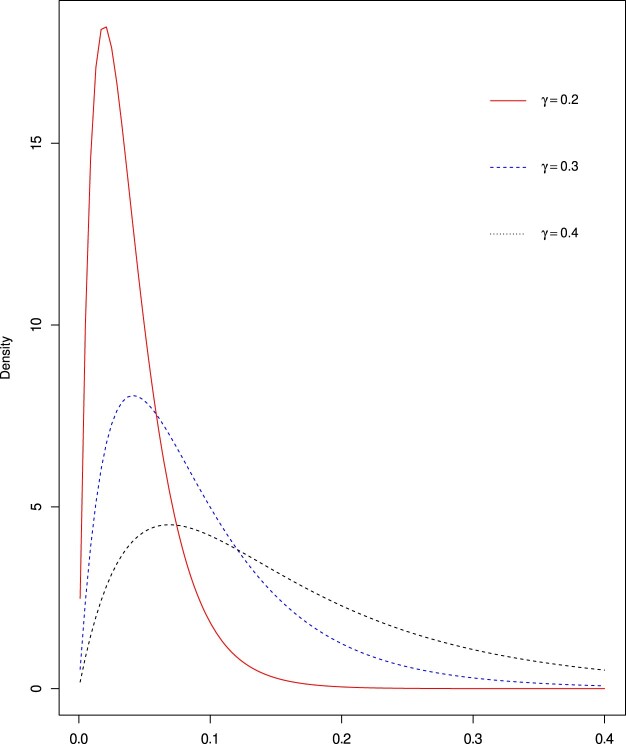
Figure 1 presents the density distribution of ${\gamma }^2$ for n = 5 and some different values of γ.

Figure 1.

The approximate density function of the ${\hat{\gamma }}^2$ for n = 5.

3. Design and implementation of the RR ${}_{r,s}-{\gamma }^2$ control chart

In the literature, the Run Rules control charts monitoring the CV have been investigated in [2] with two-sided charts. However, since the distribution of ${\gamma }^2$ is asymmetric (as can be seen from Equation (2) and also from Figure 1), these two-sided charts lead to the problem of ARL-biased (Average Run Length) performance, i.e. the out-of-control $AR{L}_1$ values are larger than the in-control values $AR{L}_0$. This problem was also pointed out in [2]. It is important to note that ARL is defined as the average number of samples before the first out-of-control point is plotted in the control chart with a given specific shift τ [17]. ARL is concerned at the zero-state of the investigated statistical measure of performance. $AR{L}_0$ and $AR{L}_1$ are denoted for the value of ARL when a process is in-control and out-of-control, respectively. It is expected that the control chart has the smallest $AR{L}_1$ value at a specific shift τ and when $AR{L}_0$ is the same for all the charts. Therefore, we overcome the ARL-biased property by designing simultaneously two one-sided charts to detect both the increase and decrease of the CV squared. In particular, we suggest defining two one-sided Run Rules control charts monitoring the CV squared, involving:

• a lower-sided r-out-of-s Run Rules control chart (denoted as RR ${}_{r,s}^{-}-{\gamma }^2$) to detect a decrease in γ with a lower control limit $LC{L}^{-}={\mu }_0\left({\hat{\gamma }}^2\right)-k_d.{\sigma }_0\left({\hat{\gamma }}^2\right)$ and an upper control limit $UC{L}^{-}=+\mathrm{\infty }$,

• an upper-sided r-out-of-s Run Rules control chart (denoted as RR ${}_{r,s}^{+}-{\gamma }^2$) to detect an increase in γ with a lower control limit $UC{L}^{+}={\mu }_0\left({\hat{\gamma }}^2\right)+k_u.{\sigma }_0\left({\hat{\gamma }}^2\right)$ and a lower control limit $LC{L}^{+}=0$,

where $k_d>0$ and $k_u>0$ are the chart parameters of the RR ${}_{r,s}^{-}-{\gamma }^2$ and RR ${}_{r,s}^{+}-{\gamma }^2$ charts, respectively.

The closed forms of ${\mu }_0\left({\hat{\gamma }}^2\right)$ and ${\sigma }_0\left({\hat{\gamma }}^2\right)$ have not been presented in the literature. We apply in this study the accurate approximations provided by Breunig [1] for both ${\mu }_0\left({\hat{\gamma }}^2\right)$ and ${\sigma }_0\left({\hat{\gamma }}^2\right)$ as follows:

$$\begin{array}{rl}{\mu }_0\left({\hat{\gamma }}^2\right)& ={\gamma }_0^2(1-\frac{3{\gamma }_0^2}{n}),\end{array}$$ (4)

$$\begin{array}{rl}{\sigma }_0\left({\hat{\gamma }}^2\right)& =\sqrt{{\gamma }_0^4\left(\frac{2}{n-1}+{\gamma }_0^2\left(\frac{4}{n}+\frac{20}{n(n-1)}+\frac{75{\gamma }_0^2}{n^2}\right)\right)-\left({\mu }_0\right({\hat{\gamma }}^2)-{\gamma }_0^2{)}^2}.\end{array}$$ (5)

Given the value of the control limit for each chart, an out-of-control signal is given at time i if r-out-of-s consecutive ${\hat{\gamma }}_i$ values are plotted outside the control interval, i.e. ${\hat{\gamma }}_i^2<LC{L}^{-}$ in the lower-sided chart and ${\hat{\gamma }}_i^2>UC{L}^{+}$ in the upper-sided chart. The control charts designed above are called pure Run Rules type chart. In this study, we only consider the 2-out-of-3, 3-out-of-4 and 4-out-of-5 Run Rules charts. The performance of the proposed charts is measured by the ARL which is calculated by using Markov chain as follows.

Firstly, we define the matrix $\mathbf{P}$ of the embedded Markov chain. For the two one-sided RR ${}_{2,3}-{\gamma }^2$ control charts, $\mathbf{P}$ is defined by

$$\mathbf{P}=\left(\begin{array}{cc}\mathbf{Q}& \mathbf{r}\\ {\mathbf{0}}^T& 1\end{array}\right)=\left(\begin{array}{cccc}0& 0& p& 1-p\\ p& 0& 0& 1-p\\ 0& 1-p& p& 0\\ 0& 0& 0& 1\end{array}\right),$$ (6)

where $\mathbf{Q}$ is a $(3,3)$ matrix of transient probabilities, $\mathbf{r}$ is a $(3,1)$ vector satisfied $\mathbf{r}=\mathbf{1}-\mathbf{Q}\mathbf{1}$ with $\mathbf{1}=(1,1,1{)}^{\mathrm{T}}$ and $\mathbf{0}=(0,0,0{)}^{\mathrm{T}}$, p is the probability that a sample drops into the control interval. The corresponding $(3,1)$ vector $\mathbf{q}$ of initial probabilities associated with the transient states is $\mathbf{q}=(0,0,1{)}^{\mathrm{T}}$, i.e. the third state is the initial state.

For the case of RR ${}_{3,4}-{\gamma }^2$ control charts, the transient probability matrix ${\mathbf{Q}}_{(7\times 7)}$ is given by

$$\mathbf{Q}=\left(\begin{array}{ccccccc}0& 0& p& 0& 0& 0& 0\\ 0& 0& 0& 0& p& 0& 0\\ 0& 0& 0& 0& 0& 1-p& p\\ p& 0& 0& 0& 0& 0& 0\\ 0& 1-p& p& 0& 0& 0& 0\\ 0& 0& 0& 1-p& p& 0& 0\\ 0& 0& 0& 0& 0& 1-p& p\end{array}\right).$$ (7)

In this case, the seventh state in the vector $\mathbf{q}=(0,0,0,0,0,0,1{)}^{\mathrm{T}}$ is the initial state.

Extended to ‘longer’ $(4,5)$ Run Rules, the $(15,15)$ matrix $\mathbf{Q}$ of transient probabilities for the two one-sided RR ${}_{4,5}-{\gamma }^2$ control charts is

$$\begin{array}{rl}\mathbf{Q}& =\left(\begin{array}{cccccccc}1-p& p& 0& 0& 0& 0& 0& p\\ 0& 0& p& 1-p& 0& 0& 0& 0\\ 0& 0& 0& 0& p& 1-p& 0& 0\\ 0& 0& 0& 0& 0& 0& 1-p& p\\ 0& 0& 0& 0& 0& 0& 0& 0\\ 0& 0& 0& 0& 0& 0& 0& 0\\ 0& 0& 0& 0& 0& 0& 0& 0\\ 0& 0& 0& 0& 0& 0& 0& 1-p\\ 0& 0& 0& 0& 0& 0& 1-p& p\\ 0& 0& 0& 0& p& 1-p& 0& 0\\ 0& 0& p& 1-p& 0& 0& 0& 0\\ 1-p& p& 0& 0& 0& 0& 0& 0\\ 0& 0& 0& 0& 0& 0& 0& 0\\ 0& 0& 0& 0& 0& 0& 0& 0\\ 0& 0& 0& 0& 0& 0& 0& 0\end{array}\right.\\ & \left.\begin{array}{ccccccc}0& 0& 0& 0& 0& 0& 0\\ 0& 0& 0& 0& 0& 0& 0\\ 0& 0& 0& 0& 0& 0& 0\\ 0& 0& 0& 0& 0& 0& 0\\ 0& 0& 0& 0& 0& 0& 1-p\\ 0& 0& 0& 0& p& 1-p& 0\\ 0& 0& 0& p& 1-p& 0& 0\\ p& 0& 0& 0& 0& 0& 0\\ 0& 0& 0& 0& 0& 0& 0\\ 0& 0& 0& 0& 0& 0& 0\\ 0& 0& 0& 0& 0& 0& 0\\ 0& 0& 0& 0& 0& 0& 0\\ 0& 1-p& p& 0& 0& 0& 0\\ 0& 0& 0& p& 1-p& 0& 0\\ 0& 0& 0& 0& 0& p& 1-p\end{array}\right),\end{array}$$ (8)

that corresponds to the $(15,1)$ initial probabilites vector $\mathbf{q}=(0,\dots ,0,1{)}^{\mathrm{T}}$ (i.e. the initial state is the 15th one). These transient probability matrices has been presented in, for example, [15–17].

Let us now suppose that the occurrence of an unexpected condition shifts the in-control CV value ${\gamma }_0$ to the out-of-control value ${\gamma }_1=\tau \times {\gamma }_0$, where $\tau >0$ is the shift size. Values of $\tau \in (0,1)$ correspond to a decrease of the ${\gamma }_0$, while values of $\tau >1$ correspond to an increase of ${\gamma }_0$. Then, the probability p is defined by

• for the RR ${}_{r,s}^{-}-{\gamma }^2$ chart:

  $$p=P({\hat{\gamma }}_i^2\ge LC{L}^{-})=1-F_{{\hat{\gamma }}^2}(LC{L}^{-}|n,{\gamma }_1),$$ (9)
• for the RR ${}_{r,s}^{+}-{\gamma }^2$ chart:

  $$p=P({\hat{\gamma }}_i^2\le UC{L}^{+})=F_{{\hat{\gamma }}^2}(UC{L}^{+}|n,{\gamma }_1),$$ (10)

where $F_{{\hat{\gamma }}^2}$ is defined in (2).

Once the matrix $\mathbf{Q}$ and the vector $\mathbf{q}$ have been determined, the ARL and the SDRL (standard deviation of run length) are calculated by

$$\begin{array}{rl}ARL& ={\mathbf{q}}^T(\mathbf{I}-\mathbf{Q}{)}^{-1}\mathbf{1},\end{array}$$ (11)

$$\begin{array}{rl}SDRL& =\sqrt{2{\mathbf{q}}^T(\mathbf{I}-\mathbf{Q}{)}^{-2}\mathbf{Q}\mathbf{1}-AR{L}^2+ARL}.\end{array}$$ (12)

It is customary that a control chart is considered to be better than its competitors if it gives a smaller value of the $AR{L}_1$ while the $AR{L}_0$ is the same. Therefore, the parameters of the RR ${}_{r,s}-{\gamma }^2$ control charts should be the solution of the following equations:

• for the RR ${}_{r,s}^{-}-{\gamma }^2$ chart:

  $$ARL(k_d,n,p,{\gamma }_0,\tau =1)=AR{L}_0,$$ (13)
• for the RR ${}_{r,s}^{+}-{\gamma }^2$ chart:

  $$ARL(k_u,n,p,{\gamma }_0,\tau =1)=AR{L}_0,$$ (14)

where $AR{L}_0$ is predefined.

4. Performance of RR ${}_{r,s}-{\gamma }^2$ control charts

Assigning the in-control value $AR{L}_0$ at $AR{L}_0=370.4$, the parameters $k_d$ and $k_u$ of the lower-sided and upper-sided RR ${}_{r,s}-{\gamma }^2$ charts for some combinations of $n\in \{5,15\},{\gamma }_0\in \{0.05,0.1,0.2\}$ are presented in Table 1. Table 2 shows the corresponding $AR{L}_1$ values of the proposed charts for various situations of the shift size τ. The obtained results show that the two one-sided RR ${}_{r,s}-{\gamma }^2$ charts not only overcome the ARL-biased problem (as the $AR{L}_1$ values are always smaller than the $AR{L}_0$) but also outperform the two-sided RR-γ charts investigated in [2]. For example, with ${\gamma }_0=0.05,\tau =1.10$ and n = 5 in the RR ${}_{2,3}-{\gamma }^2$ chart, we have $AR{L}_1=95.9$ (Table 2 in this study), which is smaller than $AR{L}_1=101.6$ (Table 2 in [2]).

Table 1. Values of the parameters $k_d$ (left side) and $k_u$ (right side) of the downward chart and the upward RR ${}_{r,s}-{\gamma }^2$ charts for ${\gamma }_0=\{0.05,0.1,0.2\}$ and $n=\{5,15\}$ when $AR{L}_0=370.4$.

	${\gamma }_0=0.05$		${\gamma }_0=0.1$		${\gamma }_0=0.2$
Charts	n = 5	n = 15	n = 5	n = 15	n = 5	n = 15
RR ${}_{2,3}-{\gamma }^2$	$(1.194,2.167)$	$(1.487,2.010)$	$(1.170,2.183)$	$(1.464,2.023)$	$(1.088,2.245)$	$(1.407,2.069)$
RR ${}_{3,4}-{\gamma }^2$	$(1.023,1.293)$	$(1.159,1.298)$	$(1.003,1.301)$	$(1.143,1.306)$	$(0.930,1.331)$	$(1.098,1.333)$
RR ${}_{4,5}-{\gamma }^2$	$(0.866,0.801)$	$(0.915,0.872)$	$(0.849,0.808)$	$(0.902,0.878)$	$(0.785,0.832)$	$(0.865,0.899)$

Table 2. Values of $(AR{L}_1,SDR{L}_1)$ of RR ${}_{r,s}-{\gamma }^2$ charts corresponding to the chart parameters in Table 1 for various situations of τ.

		${\gamma }_0=0.05$		${\gamma }_0=0.1$		${\gamma }_0=0.2$
Charts	τ	n = 5	n = 15	n = 5	n = 15	n = 5	n = 15
RR ${}_{2,3}^{-}-{\gamma }^2$	0.5	$(8.1,6.6)$	$(2.1,0.3)$	$(8.1,6.5)$	$(2.1,0.3)$	$(8.2,6.7)$	$(2.1,0.3)$
RR ${}_{3,4}^{-}-{\gamma }^2$		$(5.6,3.3)$	$(3.0,0.1)$	$(5.6,3.3)$	$(3.0,0.1)$	$(5.7,3.4)$	$(3.0,0.1)$
RR ${}_{4,5}^{-}-{\gamma }^2$		$(5.4,2.1)$	$(4.0,0.1)$	$(5.4,2.1)$	$(4.0,0.1)$	$(5.4,2.2)$	$(4.0,0.1)$
RR ${}_{2,3}^{-}-{\gamma }^2$	0.65	$(26.9,25.2)$	$(3.8,2.3)$	$(26.6,25.0)$	$(3.8,2.2)$	$(27.1,25.5)$	$(3.9,2.4)$
RR ${}_{3,4}^{-}-{\gamma }^2$		$\left(\right(16.2,13.7)$	$(3.8,1.4)$	$(16.2,13.8)$	$(3.8,1.4)$	$(16.6,14.1)$	$(3.9,1.5)$
RR ${}_{4,5}^{-}-{\gamma }^2$		$(12.6,9.5)$	$(4.5,1.0)$	$(12.7,9.6)$	$(4.5,1.0)$	$(13.0,9.9)$	$(4.5,1.0)$
RR ${}_{2,3}^{-}-{\gamma }^2$	0.8	$(87.9,86.1)$	$(17.9,16.2)$	$(87.2,85.4)$	$(17.5,15.9)$	$(88.4,86.6)$	$(18.2,16.5)$
RR ${}_{3,4}^{-}-{\gamma }^2$		$(59.8,57.1)$	$(12.6,10.2)$	$(59.9,57.2)$	$(12.7,10.3)$	$(61.1,58.4)$	$(13.2,10.8)$
RR ${}_{4,5}^{-}-{\gamma }^2$		$(46.8,43.4)$	$(11.1,8.0)$	$(47.0,43.6)$	$(11.2,8.0)$	$(48.1,44.7)$	$(11.6,8.4)$
RR ${}_{2,3}^{-}-{\gamma }^2$	0.9	$(184.4,182.5)$	$(75.4,73.7)$	$(183.7,181.9)$	$(73.9,72.2)$	$(185.2,183.4)$	$(75.7,73.9)$
RR ${}_{3,4}^{-}-{\gamma }^2$		$(149.3,146.5)$	$(55.4,52.7)$	$(149.5,146.7)$	$(55.3,52.6)$	$(151.3,148.5)$	$(57.1,54.5)$
RR ${}_{4,5}^{-}-{\gamma }^2$		$(128.7,125.1)$	$(46.5,43.1)$	$(129.1,125.4)$	$(46.7,43.3)$	$(130.9,127.3)$	$(48.3,44.9)$
RR ${}_{2,3}^{+}-{\gamma }^2$	1.10	$(95.9,94.1)$	$(45.8,44.1)$	$(96.5,94.7)$	$(46.4,44.6)$	$(98.7,96.9)$	$(48.5,46.8)$
RR ${}_{3,4}^{+}-{\gamma }^2$		$(94.2,91.5)$	$(42.3,39.7)$	$(94.8,92.0)$	$(42.8,40.1)$	$(97.0,94.2)$	$(44.7,42.1)$
RR ${}_{4,5}^{+}-{\gamma }^2$		$(94.9,91.4)$	$(41.3,37.9)$	$(95.4,91.9)$	$(41.7,38.3)$	$(97.6,94.0)$	$(43.6,40.2)$
RR ${}_{2,3}^{+}-{\gamma }^2$	1.25	$(25.8,24.2)$	$(8.7,7.1)$	$(26.1,24.4)$	$(8.8,7.2)$	$(27.2,25.6)$	$(9.4,7.8)$
RR ${}_{3,4}^{+}-{\gamma }^2$		$(26.3,23.8)$	$(8.9,6.5)$	$(26.5,24.0)$	$(9.0,6.6)$	$(27.6,25.1)$	$(9.5,7.1)$
RR ${}_{4,5}^{+}-{\gamma }^2$		$(27.5,24.2)$	$(9.5,6.4)$	$(27.8,24.5)$	$(9.6,6.5)$	$(28.9,25.5)$	$(10.1,7.0)$
RR ${}_{2,3}^{+}-{\gamma }^2$	1.5	$(8.1,6.6)$	$(3.1,1.5)$	$(8.2,6.7)$	$(3.1,1.6)$	$(8.6,7.1)$	$(3.3,1.7)$
RR ${}_{3,4}^{+}-{\gamma }^2$		$(9.1,6.7)$	$(3.9,1.4)$	$(9.2,6.8)$	$(3.9,1.5)$	$(9.6,7.2)$	$(4.0,1.6)$
RR ${}_{4,5}^{+}-{\gamma }^2$		$(10.2,7.1)$	$(4.8,1.4)$	$(10.3,7.2)$	$(4.8,1.4)$	$(10.7,7.6)$	$(4.9,1.6)$
RR ${}_{2,3}^{+}-{\gamma }^2$	2.0	$(3.4,1.9)$	$(2.1,0.3)$	$(3.4,1.9)$	$(2.1,0.3)$	$(3.6,2.1)$	$(2.1,0.4)$
RR ${}_{3,4}^{+}-{\gamma }^2$		$(4.3,2.0)$	$(3.1,0.3)$	$(4.4,2.0)$	$(3.1,0.3)$	$(4.6,2.2)$	$(3.1,0.3)$
RR ${}_{4,5}^{+}-{\gamma }^2$		$(5.3,2.1)$	$(4.0,0.2)$	$(5.4,2.1)$	$(4.0,0.2)$	$(5.6,2.3)$	$(4.1,0.3)$

5. Linear covariate error model for the coefficient of variation

The previous design for the RR ${}_{r,s}-{\gamma }^2$ control charts is based on a latent assumption that the values in the collected sample are measured exactly without the measurement error. This assumption, however, is usually not reached in practice and it is difficult to avoid the measurement error. In this section, we suppose a linear covariate error model to the measurement error, which is suggested by Linna and Woodall [9].

Suppose that the quality characteristic X of n consecutive items at step ith is $(X_{i,1},X_{i,2},\dots ,X_{i,n})$, where $X_{i,j}\sim N({\mu }_0+a{\sigma }_0,b^2{\sigma }_0^2),$ where ${\mu }_0$ and ${\sigma }_0$ are the in-control mean and standard deviation of X, a and b represent the standardized mean and the standardized deviation shifts, respectively. The process has shifted if the process mean ${\mu }_0$ and/or the process standard deviation ${\sigma }_0$ have changed ( $a\ne 0$ and/or $b\ne 1$). Due to the measurement error, we only observe the values $(X_{i,j,1}^{\ast },\dots ,X_{i,j,m}^{\ast })$ of a set of m measurement operations instead the true values $X_{i,j}$. According to the linear covariate error model, we assume $X_{i,j,k}^{\ast }=A+B{X}_{i,j}+{\epsilon }_{i,j,k}$, where A and B are two known constants and ${\epsilon }_{i,j,k}$ is a normal random error term with parameters $(0,{\mathrm{\Sigma }}_M)$ and independent of $X_{i,j}$. Note that A is the constant bias component and B represents the parameter modeling the linearity error. The bias and linearity errors are monitored and possibly eliminated by means of a gauge calibration, see the AIAG manual [6] for further details.

Let ${\overline{X}}_{i,j}^{\ast }$ denote the mean of m observed quantities of the same item j at the $i\mathrm{t}\mathrm{h}$ sampling. It is straightforward to show that

$${\overline{X}}_{i,j}^{\ast }\sim N({\mu }^{\ast },{\sigma }^{\ast 2})=N\left(A+B({\mu }_0+a{\sigma }_0),B^2{b}^2{\sigma }_0^2+\frac{{\sigma }_M^2}{m}\right).$$

Tran et al. [19] showed that the CV of the quantity ${\overline{X}}_{i,j}^{\ast }$ is

$${\gamma }^{\ast }=\frac{{\sigma }^{\ast }}{{\mu }^{\ast }}=\frac{\sqrt{B^2{b}^2+\frac{{\eta }^2}{m}}}{\theta +B(1+a{\gamma }_0)}\times {\gamma }_0,$$ (15)

where ${\gamma }_0={\sigma }_0/{\mu }_0,\eta ={\sigma }_M/{\sigma }_0$ and $\theta =A/{\mu }_0$ are the in-control value of CV, the precision and the accuracy error ratios, respectively. The sample coefficient of variation ${\hat{\gamma }}_i^{\ast }$ is defined by ${\hat{\gamma }}_i^{\ast }=S_i^{\ast }/{\overline{\overline{X}}}_i^{\ast }$ where ${\overline{\overline{X}}}_i^{\ast }$ and $S_i^{\ast }$ are the sample mean and standard deviation of ${\overline{X}}_{1,j}^{\ast },\dots ,{\overline{X}}_{n,j}^{\ast }$ ${\overline{X}}_{1,j}^{\ast },\dots ,{\overline{X}}_{n,j}^{\ast },$ i.e.

$${\overline{\overline{X}}}_i^{\ast }=\frac{1}{n}\sum _{j=1}^n{\overline{X}}_{i,j}^{\ast }\mathrm{a}\mathrm{n}\mathrm{d}{S}_i^{\ast }=\sqrt{\frac{1}{n-1}\sum _{j=1}^n({\overline{X}}_{i,j}^{\ast }-{\overline{\overline{X}}}_i^{\ast }{)}^2}.$$

The c.d.f of ${\hat{\gamma }}^{\ast 2}$ can be obtained from (2) by simply replacing γ by ${\gamma }^{\ast }$, i.e. the c.d.f $F_{{\hat{\gamma }}^{\ast 2}}(x|n,{\gamma }^{\ast })$ of ${\hat{\gamma }}^{\ast 2}$ is given by

$$F_{{\hat{\gamma }}^{\ast 2}}(x|n,{\gamma }^{\ast })=1-F_F\left(\frac{n}{x}\left|1,n-1,\frac{n}{{\gamma }^{\ast 2}}\right.\right).$$ (16)

6. Implementation and the performance of the RR ${}_{r,s}-{\gamma }^2$ charts with measurement errors

Under the presence of measurement errors, the values ${\mu }_0\left({\hat{\gamma }}^{\ast 2}\right)$ and ${\sigma }_0\left({\hat{\gamma }}^{\ast 2}\right)$ are calculated as in (4) and (5), where ${\gamma }_0$ is replaced by ${\gamma }_0^{\ast }$, which is defined from (15) with a = 0 and b = 1:

$${\gamma }_0^{\ast }=\frac{\sqrt{B^2+\frac{{\eta }^2}{m}}}{\theta +B}\times {\gamma }_0.$$ (17)

Suppose that the in-control value ${\gamma }_0$ is shifted to the out-of-control value ${\gamma }_1$ with the size τ, we can represent τ according to a and b as $\tau =b/(1+a{\gamma }_0)$. Therefore, the out-of-control CV of the observed quantity ${\overline{X}}_{i,j}^{\ast }$ can be expressed by

$${\gamma }_1^{\ast }=\frac{\sqrt{B^2{b}^2+\frac{{\eta }^2}{m}}}{\theta +\frac{Bb}{\tau }}\times {\gamma }_0.$$ (18)

In the implementation of RR ${}_{r,s}-{\gamma }^2$ control charts, the control limits, $UC{L}^{\ast +}={\mu }_0\left({\hat{\gamma }}^{\ast 2}\right)+k_u^{\ast }.{\sigma }_0\left({\hat{\gamma }}^{\ast 2}\right)$ and $LC{L}^{\ast -}={\mu }_0\left({\hat{\gamma }}^{\ast 2}\right)-k_d^{\ast }.{\sigma }_0\left({\hat{\gamma }}^{\ast 2}\right)$, are also found by solving the chart parameters $k_d$ and $k_u$ as the solution of the following equations:

• for the RR ${}_{r,s}^{-}-{\gamma }^2$ chart:

  $$ARL(k_d,n,p,{\gamma }_0,\theta ,\eta ,m,B,b)=AR{L}_0,$$ (19)
• for the RR ${}_{r,s}^{+}-{\gamma }^2$ chart:

  $$ARL(k_u,n,p,{\gamma }_0,\theta ,\eta ,m,B,b)=AR{L}_0.$$ (20)

The ARL in (19) and (20) should be calculated with the transition probability matrix $\mathbf{Q}$ where the transition probability p is defined from (9) and (10) but with the c.d.f $F_{{\hat{\gamma }}^{\ast 2}}(x|n,{\gamma }^{\ast })$ of ${\hat{\gamma }}^{\ast 2}$ in (16) instead of c.d.f $F_{{\hat{\gamma }}^2}$ in (2).

To investigate the performance of the RR ${}_{r,s}-{\gamma }^2$ charts under the appearance of the measurement error, we consider several possible values of the parameters: $n\in \{5,15\}$, ${\gamma }_0\in \{0.05,0.1,0.2\}$, $\eta \in \{0,0.1,0.2,0.3,0.5,1\}$, $\theta \in \{0,0.01,0.02,0.03,0.04,0.05\}$, $m\in \{1,3,5,7,10\}$ and $B\in \{0.8,0.9,1,1.1,1.2\}$. The value of B is considered within the range $[0.8,1.2]$ according to the guidelines for measurement system acceptability presented in manual of AIA Group [6] for measurement system analysis. Without loss of generality, we assume in the remaining that b = 1. The in-control value CV is also set at $AR{L}_0=370.4$.

The control limits of the proposed charts for some specific values of these parameters have been presented in Table 3. The other values of the control limits for other situations of these parameters are not presented here but are available upon request from authors.

Table 3. Values of LCL (first row) and UCL (second row) for the RR ${}_{r,s}-{\gamma }^2$ control charts in the presence of measurement errors, for different values of η, θ, n, ${\gamma }_0$, B = 1 and m = 1.

			RR ${}_{2,3}-{\gamma }^2$		RR ${}_{3,4}-{\gamma }^2$		RR ${}_{3,4}-{\gamma }^2$
η	θ	${\gamma }_0$	n = 10	n = 15	n = 10	n = 15	n = 10	n = 15
0.1	0.01	0.05	0.0004	0.0011	0.0007	0.0014	0.0009	0.0016
			0.0063	0.0044	0.0047	0.0037	0.0039	0.0033
		0.10	0.0015	0.0043	0.0027	0.0055	0.0038	0.0065
			0.0254	0.0175	0.0191	0.0148	0.0156	0.0132
			0.0582	0.0399	0.0435	0.0336	0.0354	0.0299
		0.20	0.0059	0.0172	0.0107	0.0220	0.0151	0.0257
			0.1061	0.0718	0.0786	0.0602	0.0636	0.0534
0.28	0.05	0.05	0.0004	0.0011	0.0007	0.0014	0.0009	0.0016
			0.0062	0.0043	0.0047	0.0036	0.0038	0.0033
		0.10	0.0015	0.0043	0.0027	0.0055	0.0037	0.0064
			0.0251	0.0173	0.0189	0.0146	0.0154	0.0130
			0.0575	0.0394	0.0430	0.0332	0.0350	0.0295
		0.20	0.0059	0.0170	0.0106	0.0218	0.0149	0.0254
			0.1047	0.0709	0.0776	0.0595	0.0629	0.0528

Tables 4–7 show the corresponding values of the $AR{L}_1$ under different effects of the parameters $\eta ,\theta ,m$ and B of the linear covariate model. Some simple conclusions can be drawn from these tables as follows:

• The increase of the precision error ratio η leads to an increase of the $AR{L}_1$. However, this increase in the $AR{L}_1$ following the change of η is not significant, especially when $\eta ⩽0.3$. For example, for the RR ${}_{2,3}-{\gamma }^2$ chart with $n=5,{\gamma }_0=0.05,B=1,m=1,\theta =0.05$ and $\tau =0.8$, we have $AR{L}_1=93.12$ when $\eta =0.0$ and $AR{L}_1=93.20$ when $\eta =0.3$ (Table 4). That means the precision error ratio does not affect much the performance of the proposed charts.

• The accuracy error θ has a negative impact on the RR ${}_{r,s}-{\gamma }^2$ charts' performance: the larger the accuracy error θ is, the larger the value $AR{L}_1$ is, i.e. the lower of the control chart is in detecting the out-of-control condition. For example, in the RR ${}_{3,4}-{\gamma }^2$ chart with $n=5,{\gamma }_0=0.1,B=1,m=1,\eta =0.28$ and $\tau =1.3$, we have $AR{L}_1=26.56$ when $\theta =0.0$ and $AR{L}_1=29.19$ when $\theta =0.5$ (Table 5).

• Given the value of other parameters, the variation of B significantly affects the performance of the RR ${}_{r,s}-{\gamma }^2$ charts. For instance, in Table 6 with the RR ${}_{4,5}^{-}-{\gamma }^2$ control chart and $n=5,m=1,{\gamma }_0=0.2,\eta =0.28,\theta =0.05,\tau =0.7$ we have $AR{L}_1=14.43$ when B = 0.8 and $AR{L}_1=13.93$ when B = 1.2.

• In many situations, taking multiple measurements per item in each sample is an alternative to compensate for the effect of the measurement error. However, the obtained results in this study show that this is not an effective way to reduce the impact of measurement errors on the proposed control charts performance. This is because, according to the results of the numerical analysis, the $AR{L}_1$ decreases trivially or is almost unchanged when m increases from m = 1 to m = 10. For example, with $n=5,B=1,{\gamma }_0=0.05,\eta =0.28,\theta =0.05,\tau =0.8$ in the RR ${}_{2,3}^{+}-{\gamma }^2,$ we have $AR{L}_1=9.07$ for both m = 1 and m = 10 (Table 7). Hence, in order to reduce the impact of ME on the proposed control charts performance, we can improve the measurement system to reduce the values of θ and η.

• In general, the RR ${}_{r,s}-{\gamma }^2$ control charts give better performance in detecting the small process shifts compared to the VSI- ${\gamma }^2$ control chart investigated in [11], under the same condition of measurement errors. For example, with the same values of $n=5,{\gamma }_0=0.05,\eta =0.28,\theta =0.05,\tau =0.8$, we have $AR{L}_1=46.80$ for the RR ${}_{4,5}-{\gamma }^2$ (Table 5 in this study), which is smaller than $AR{L}_1=61.99$ for the VSI ${\gamma }^2$ control chart with $(h_S,h_L)=0.1,4.0$ (Table 10 in [11]).

Table 4. The ARL values of the RR ${}_{r,s}-{\gamma }^2$ control charts in the presence of measurement errors for ${\gamma }_0=0.05$ (left side), ${\gamma }_0=0.1$ (middle) and ${\gamma }_0=0.2$ (right side), and for different values of η, $\theta =0.05$, τ, n, B = 1, m = 1.

Charts	τ	$\eta =0$	$\eta =0.1$	$\eta =0.2$	$\eta =0.3$	$\eta =0.5$	$\eta =1$
n = 5
RR ${}_{2,3}-{\gamma }^2$	0.5	$(8.92,8.85,8.98)$	$(8.94,8.85,8.99)$	$(8.92,8.84,8.99)$	$(8.92,8.86,9.01)$	$(8.90,8.84,9.06)$	$(8.87,8.87,9.24)$
	0.7	$(29.38,29.11,29.54)$	$(29.45,29.14,29.58)$	$(29.35,29.06,29.57)$	$(29.40,29.13,29.65)$	$(29.29,29.09,29.80)$	$(29.19,29.18,30.42)$
	0.8	$(93.12,92.52,93.41)$	$(93.28,92.44,93.58)$	$(93.15,92.24,93.38)$	$(93.20,92.54,93.68)$	$(92.90,92.39,93.98)$	$(92.74,92.60,95.22)$
	1.3	$(28.57,28.83,29.93)$	$(28.57,28.84,29.94)$	$(28.57,28.85,29.99)$	$(28.58,28.87,30.06)$	$(28.59,28.92,30.30)$	$(28.66,29.19,31.45)$
	1.5	$(9.07,9.17,9.62)$	$(9.07,9.17,9.62)$	$(9.07,9.18,9.64)$	$(9.07,9.19,9.67)$	$(9.07,9.21,9.77)$	$(9.10,9.32,10.24)$
	2.0	$(3.70,3.74,3.92)$	$(3.70,3.74,3.92)$	$(3.70,3.74,3.92)$	$(3.70,3.75,3.94)$	$(3.70,3.76,3.98)$	$(3.71,3.80,4.16)$
RR ${}_{3,4}-{\gamma }^2$	0.5	$(6.01,6.02,6.11)$	$(6.02,6.02,6.12)$	$(6.02,6.02,6.12)$	$(6.01,6.02,6.13)$	$(6.01,6.02,6.15)$	$(6.01,6.05,6.26)$
	0.7	$(17.69,17.71,18.09)$	$(17.71,17.71,18.11)$	$(17.71,17.71,18.11)$	$(17.70,17.73,18.15)$	$(17.71,17.73,18.25)$	$(17.68,17.82,18.68)$
	0.8	$(64.10,64.21,65.33)$	$(64.20,64.19,65.35)$	$(64.22,64.17,65.37)$	$(64.13,64.24,65.47)$	$(64.22,64.25,65.78)$	$(64.07,64.48,67.06)$
	1.3	$(28.92,29.17,30.21)$	$(28.92,29.17,30.22)$	$(28.92,29.18,30.26)$	$(28.93,29.20,30.34)$	$(28.93,29.25,30.56)$	$(29.00,29.51,31.63)$
	1.5	$(10.01,10.12,10.55)$	$(10.01,10.12,10.55)$	$(10.01,10.12,10.57)$	$(10.02,10.13,10.60)$	$(10.02,10.15,10.69)$	$(10.05,10.26,11.14)$
	2.0	$(4.67,4.71,4.89)$	$(4.67,4.71,4.89)$	$(4.67,4.72,4.90)$	$(4.67,4.72,4.91)$	$(4.68,4.73,4.95)$	$(4.69,4.77,5.13)$
RR ${}_{4,5}-{\gamma }^2$	0.5	$(5.64,5.65,5.71)$	$(5.64,5.65,5.71)$	$(5.64,5.65,5.72)$	$(5.64,5.65,5.72)$	$(5.64,5.65,5.74)$	$(5.64,5.67,5.81)$
	0.7	$(13.75,13.79,14.09)$	$(13.76,13.80,14.10)$	$(13.76,13.81,14.12)$	$(13.75,13.81,14.13)$	$(13.76,13.81,14.20)$	$(13.76,13.89,14.52)$
	0.8	$(50.44,50.60,51.63)$	$(50.49,50.63,51.67)$	$(50.51,50.66,51.74)$	$(50.45,50.66,51.78)$	$(50.46,50.67,52.03)$	$(50.48,50.96,53.14)$
	1.3	$(30.17,30.42,31.45)$	$(30.18,30.43,31.46)$	$(30.19,30.43,31.51)$	$(30.18,30.45,31.57)$	$(30.20,30.51,31.80)$	$(30.25,30.76,32.85)$
	1.5	$(11.17,11.27,11.70)$	$(11.17,11.27,11.71)$	$(11.17,11.27,11.73)$	$(11.17,11.28,11.76)$	$(11.17,11.30,11.85)$	$(11.20,11.41,12.30)$
	2.0	$(5.68,5.72,5.90)$	$(5.68,5.72,5.90)$	$(5.68,5.72,5.91)$	$(5.68,5.72,5.92)$	$(5.68,5.73,5.96)$	$(5.69,5.78,6.14)$
n = 15
RR ${}_{2,3}-{\gamma }^2$	0.5	$(2.12,2.12,2.13)$	$(2.12,2.12,2.13)$	$(2.12,2.12,2.13)$	$(2.12,2.12,2.13)$	$(2.12,2.12,2.14)$	$(2.12,2.12,2.15)$
	0.7	$(4.12,4.08,4.18)$	$(4.12,4.08,4.18)$	$(4.12,4.08,4.18)$	$(4.11,4.08,4.19)$	$(4.11,4.08,4.22)$	$(4.09,4.10,4.35)$
	0.8	$(19.86,19.42,19.97)$	$(19.83,19.43,20.02)$	$(19.83,19.45,20.02)$	$(19.80,19.45,20.06)$	$(19.73,19.43,20.20)$	$(19.56,19.55,21.01)$
	1.3	$(9.68,9.81,10.41)$	$(9.68,9.82,10.41)$	$(9.68,9.82,10.44)$	$(9.68,9.83,10.48)$	$(9.69,9.86,10.61)$	$(9.72,10.01,11.22)$
	1.5	$(3.32,3.36,3.52)$	$(3.32,3.36,3.52)$	$(3.32,3.36,3.53)$	$(3.32,3.36,3.54)$	$(3.32,3.37,3.58)$	$(3.33,3.41,3.75)$
	2.0	$(2.13,2.14,2.17)$	$(2.13,2.14,2.17)$	$(2.13,2.14,2.18)$	$(2.13,2.14,2.18)$	$(2.13,2.14,2.19)$	$(2.13,2.15,2.23)$
RR ${}_{3,4}-{\gamma }^2$	0.5	$(3.02,3.02,3.03)$	$(3.02,3.02,3.03)$	$(3.02,3.02,3.03)$	$(3.02,3.02,3.03)$	$(3.02,3.02,3.03)$	$(3.02,3.03,3.03)$
	0.7	$(4.02,4.02,4.09)$	$(4.02,4.02,4.09)$	$(4.01,4.02,4.10)$	$(4.01,4.02,4.10)$	$(4.01,4.03,4.12)$	$(4.01,4.04,4.20)$
	0.8	$(13.91,13.92,14.41)$	$(13.92,13.91,14.42)$	$(13.90,13.91,14.44)$	$(13.90,13.92,14.48)$	$(13.89,13.95,14.59)$	$(13.87,14.06,15.13)$
	1.3	$(9.77,9.89,10.42)$	$(9.77,9.90,10.42)$	$(9.78,9.90,10.44)$	$(9.78,9.91,10.48)$	$(9.78,9.94,10.59)$	$(9.81,10.07,11.13)$
	1.5	$(4.10,4.13,4.28)$	$(4.10,4.13,4.28)$	$(4.10,4.14,4.29)$	$(4.10,4.14,4.30)$	$(4.10,4.14,4.33)$	$(4.11,4.18,4.48)$
	2.0	$(3.09,3.10,3.12)$	$(3.09,3.10,3.13)$	$(3.09,3.10,3.13)$	$(3.09,3.10,3.13)$	$(3.09,3.10,3.14)$	$(3.09,3.11,3.17)$
RR ${}_{4,5}-{\gamma }^2$	0.5	$(4.01,4.01,4.01)$	$(4.01,4.01,4.01)$	$(4.01,4.01,4.01)$	$(4.01,4.01,4.01)$	$(4.01,4.01,4.01)$	$(4.01,4.01,4.01)$
	0.7	$(4.58,4.59,4.64)$	$(4.58,4.59,4.64)$	$(4.58,4.59,4.64)$	$(4.58,4.59,4.65)$	$(4.58,4.59,4.66)$	$(4.58,4.60,4.71)$
	0.8	$(12.09,12.14,12.55)$	$(12.09,12.14,12.56)$	$(12.09,12.14,12.58)$	$(12.09,12.15,12.61)$	$(12.09,12.17,12.70)$	$(12.09,12.27,13.15)$
	1.3	$(10.37,10.48,10.97)$	$(10.37,10.48,10.98)$	$(10.37,10.49,11.00)$	$(10.37,10.49,11.03)$	$(10.38,10.52,11.14)$	$(10.40,10.64,11.64)$
	1.5	$(4.97,5.00,5.13)$	$(4.97,5.00,5.13)$	$(4.97,5.00,5.14)$	$(4.97,5.00,5.15)$	$(4.97,5.01,5.18)$	$(4.98,5.04,5.32)$
	2.0	$(4.07,4.08,4.10)$	$(4.07,4.08,4.10)$	$(4.07,4.08,4.10)$	$(4.07,4.08,4.10)$	$(4.07,4.08,4.11)$	$(4.07,4.08,4.13)$

Table 7. The ARL values of the RR ${}_{r,s}-{\gamma }^2$ control charts in the presence of measurement errors for ${\gamma }_0=0.05$ (left side), ${\gamma }_0=0.1$ (middle) and ${\gamma }_0=0.2$ (right side), and for different values of m, τ, n, $\eta =0.28$, $\theta =0.05$, B = 1.

Charts	τ	m = 1	m = 3	m = 5	m = 7	m = 10
n = 5
RR ${}_{2,3}-{\gamma }^2$	0.5	$(8.93,8.85,9.01)$	$(8.92,8.84,8.99)$	$(8.93,8.84,8.99)$	$(8.94,8.85,8.99)$	$(8.93,8.84,8.99)$
	0.7	$(29.42,29.13,29.64)$	$(29.39,29.06,29.56)$	$(29.41,29.09,29.56)$	$(29.42,29.11,29.58)$	$(29.39,29.07,29.58)$
	0.8	$(93.24,92.53,93.63)$	$(93.00,92.20,93.47)$	$(93.22,92.44,93.43)$	$(93.20,92.50,93.57)$	$(93.12,92.23,93.52)$
	1.3	$(28.58,28.86,30.04)$	$(28.57,28.84,29.96)$	$(28.57,28.84,29.95)$	$(28.57,28.83,29.95)$	$(28.57,28.83,29.94)$
	1.5	$(9.07,9.18,9.66)$	$(9.07,9.18,9.63)$	$(9.07,9.17,9.62)$	$(9.07,9.17,9.62)$	$(9.07,9.17,9.62)$
	2.0	$(3.70,3.75,3.93)$	$(3.70,3.74,3.92)$	$(3.70,3.74,3.92)$	$(3.70,3.74,3.92)$	$(3.70,3.74,3.92)$
RR ${}_{3,4}-{\gamma }^2$	0.5	$(6.01,6.02,6.12)$	$(6.02,6.02,6.12)$	$(6.01,6.01,6.12)$	$(6.02,6.02,6.12)$	$(6.01,6.02,6.12)$
	0.7	$(17.70,17.72,18.14)$	$(17.72,17.70,18.11)$	$(17.70,17.69,18.11)$	$(17.71,17.71,18.10)$	$(17.69,17.71,18.11)$
	0.8	$(64.20,64.24,65.45)$	$(64.26,64.15,65.33)$	$(64.18,64.15,65.36)$	$(64.18,64.21,65.35)$	$(64.15,64.15,65.39)$
	1.3	$(28.92,29.19,30.31)$	$(28.92,29.17,30.25)$	$(28.92,29.17,30.23)$	$(28.92,29.17,30.22)$	$(28.92,29.17,30.22)$
	1.5	$(10.02,10.13,10.59)$	$(10.01,10.12,10.56)$	$(10.01,10.12,10.55)$	$(10.01,10.12,10.55)$	$(10.01,10.12,10.55)$
	2.0	$(4.67,4.72,4.91)$	$(4.67,4.72,4.89)$	$(4.67,4.71,4.89)$	$(4.67,4.71,4.89)$	$(4.67,4.71,4.89)$
RR ${}_{4,5}-{\gamma }^2$	0.5	$(5.64,5.65,5.72)$	$(5.64,5.65,5.71)$	$(5.64,5.65,5.71)$	$(5.64,5.65,5.71)$	$(5.64,5.65,5.71)$
	0.7	$(13.76,13.80,14.13)$	$(13.76,13.80,14.10)$	$(13.75,13.80,14.10)$	$(13.76,13.79,14.10)$	$(13.75,13.79,14.10)$
	0.8	$(50.47,50.63,51.74)$	$(50.50,50.65,51.67)$	$(50.46,50.62,51.68)$	$(50.48,50.58,51.67)$	$(50.47,50.60,51.67)$
	1.3	$(30.19,30.44,31.56)$	$(30.18,30.43,31.49)$	$(30.18,30.43,31.47)$	$(30.18,30.42,31.46)$	$(30.17,30.42,31.46)$
	1.5	$(11.17,11.28,11.75)$	$(11.17,11.27,11.72)$	$(11.17,11.27,11.71)$	$(11.17,11.27,11.71)$	$(11.17,11.27,11.71)$
	2.0	$(5.68,5.72,5.91)$	$(5.68,5.72,5.90)$	$(5.68,5.72,5.90)$	$(5.68,5.72,5.90)$	$(5.68,5.72,5.90)$
n = 15
RR ${}_{2,3}-{\gamma }^2$	0.5	$(2.12,2.12,2.13)$	$(2.12,2.12,2.13)$	$(2.12,2.12,2.13)$	$(2.12,2.12,2.13)$	$(2.12,2.12,2.13)$
	0.7	$(4.12,4.08,4.19)$	$(4.12,4.08,4.18)$	$(4.12,4.08,4.18)$	$(4.12,4.08,4.18)$	$(4.12,4.08,4.18)$
	0.8	$(19.82,19.40,20.05)$	$(19.83,19.41,19.99)$	$(19.86,19.45,20.00)$	$(19.85,19.45,20.00)$	$(19.84,19.43,19.98)$
	1.3	$(9.68,9.83,10.47)$	$(9.68,9.82,10.43)$	$(9.68,9.82,10.42)$	$(9.68,9.82,10.42)$	$(9.68,9.82,10.41)$
	1.5	$(3.32,3.36,3.54)$	$(3.32,3.36,3.53)$	$(3.32,3.36,3.52)$	$(3.32,3.36,3.52)$	$(3.32,3.36,3.52)$
	2.0	$(2.13,2.14,2.18)$	$(2.13,2.14,2.17)$	$(2.13,2.14,2.17)$	$(2.13,2.14,2.17)$	$(2.13,2.14,2.17)$
RR ${}_{3,4}-{\gamma }^2$	0.5	$(3.02,3.02,3.03)$	$(3.02,3.02,3.03)$	$(3.02,3.02,3.03)$	$(3.02,3.02,3.03)$	$(3.02,3.02,3.03)$
	0.7	$(4.02,4.02,4.10)$	$(4.02,4.02,4.10)$	$(4.01,4.02,4.09)$	$(4.02,4.02,4.09)$	$(4.01,4.02,4.09)$
	0.8	$(13.91,13.92,14.46)$	$(13.90,13.92,14.44)$	$(13.90,13.91,14.42)$	$(13.92,13.90,14.42)$	$(13.91,13.90,14.42)$
	1.3	$(9.78,9.91,10.47)$	$(9.78,9.90,10.44)$	$(9.78,9.90,10.43)$	$(9.78,9.90,10.42)$	$(9.78,9.90,10.42)$
	1.5	$(4.10,4.14,4.29)$	$(4.10,4.13,4.28)$	$(4.10,4.13,4.28)$	$(4.10,4.13,4.28)$	$(4.10,4.13,4.28)$
	2.0	$(3.09,3.10,3.13)$	$(3.09,3.10,3.13)$	$(3.09,3.10,3.13)$	$(3.09,3.10,3.13)$	$(3.09,3.10,3.13)$
RR ${}_{4,5}-{\gamma }^2$	0.5	$(4.01,4.01,4.01)$	$(4.01,4.01,4.01)$	$(4.01,4.01,4.01)$	$(4.01,4.01,4.01)$	$(4.01,4.01,4.01)$
	0.7	$(4.58,4.59,4.64)$	$(4.58,4.59,4.64)$	$(4.58,4.59,4.64)$	$(4.58,4.59,4.64)$	$(4.58,4.59,4.64)$
	0.8	$(12.09,12.14,12.60)$	$(12.09,12.14,12.57)$	$(12.09,12.14,12.57)$	$(12.09,12.14,12.56)$	$(12.09,12.14,12.56)$
	1.3	$(10.37,10.49,11.02)$	$(10.37,10.48,10.99)$	$(10.37,10.48,10.98)$	$(10.37,10.48,10.98)$	$(10.37,10.48,10.98)$
	1.5	$(4.97,5.00,5.15)$	$(4.97,5.00,5.14)$	$(4.97,5.00,5.14)$	$(4.97,5.00,5.13)$	$(4.97,5.00,5.13)$
	2.0	$(4.07,4.08,4.10)$	$(4.07,4.08,4.10)$	$(4.07,4.08,4.10)$	$(4.07,4.08,4.10)$	$(4.07,4.08,4.10)$

Table 5. The ARL values of the RR ${}_{r,s}-{\gamma }^2$ control charts in the presence of measurement errors for ${\gamma }_0=0.05$ (left side), ${\gamma }_0=0.1$ (middle) and ${\gamma }_0=0.2$ (right side), and for different values of θ, $\eta =0.28$, τ, n, B = 1, m = 1.

Charts	τ	$\theta =0$	$\theta =0.01$	$\theta =0.02$	$\theta =0.03$	$\theta =0.04$	$\theta =0.05$
n = 5
RR ${}_{2,3}-{\gamma }^2$	0.5	$(8.11,8.06,8.22)$	$(8.28,8.21,8.38)$	$(8.43,8.35,8.53)$	$(8.59,8.52,8.69)$	$(8.75,8.69,8.84)$	$(8.93,8.85,9.01)$
	0.7	$(26.88,26.65,27.19)$	$(27.38,27.15,27.71)$	$(27.87,27.55,28.15)$	$(28.36,28.10,28.66)$	$(28.87,28.62,29.12)$	$(29.42,29.13,29.64)$
	0.8	$(87.72,87.23,88.36)$	$(88.96,88.30,89.56)$	$(89.94,89.12,90.51)$	$(90.85,90.33,91.69)$	$(91.95,91.30,92.44)$	$(93.24,92.53,93.63)$
	1.3	$(25.84,26.13,27.35)$	$(26.38,26.67,27.88)$	$(26.93,27.21,28.42)$	$(27.47,27.76,28.96)$	$(28.02,28.31,29.50)$	$(28.58,28.86,30.04)$
	1.5	$(8.09,8.20,8.68)$	$(8.28,8.39,8.87)$	$(8.47,8.59,9.07)$	$(8.67,8.78,9.26)$	$(8.87,8.98,9.46)$	$(9.07,9.18,9.66)$
	2.0	$(3.38,3.42,3.61)$	$(3.44,3.48,3.67)$	$(3.50,3.55,3.73)$	$(3.57,3.61,3.80)$	$(3.63,3.68,3.87)$	$(3.70,3.75,3.93)$
RR ${}_{3,4}-{\gamma }^2$	0.5	$(5.60,5.61,5.71)$	$(5.68,5.69,5.80)$	$(5.76,5.77,5.88)$	$(5.84,5.85,5.96)$	$(5.93,5.93,6.04)$	$(6.01,6.02,6.12)$
	0.7	$(16.15,16.20,16.62)$	$(16.47,16.50,16.93)$	$(16.76,16.78,17.24)$	$(17.07,17.10,17.53)$	$(17.38,17.40,17.84)$	$(17.70,17.72,18.14)$
	0.8	$(59.75,59.92,61.22)$	$(60.70,60.79,62.12)$	$(61.56,61.53,63.02)$	$(62.38,62.49,63.79)$	$(63.26,63.35,64.67)$	$(64.20,64.24,65.45)$
	1.3	$(26.28,26.56,27.72)$	$(26.80,27.08,28.23)$	$(27.33,27.60,28.75)$	$(27.86,28.13,29.27)$	$(28.39,28.66,29.79)$	$(28.92,29.19,30.31)$
	1.5	$(9.05,9.16,9.63)$	$(9.24,9.35,9.82)$	$(9.43,9.54,10.01)$	$(9.62,9.73,10.20)$	$(9.82,9.93,10.39)$	$(10.02,10.13,10.59)$
	2.0	$(4.35,4.39,4.58)$	$(4.41,4.46,4.64)$	$(4.48,4.52,4.70)$	$(4.54,4.58,4.77)$	$(4.61,4.65,4.84)$	$(4.67,4.72,4.91)$
RR ${}_{4,5}-{\gamma }^2$	0.5	$(5.37,5.39,5.46)$	$(5.43,5.44,5.51)$	$(5.48,5.49,5.56)$	$(5.53,5.54,5.61)$	$(5.58,5.59,5.67)$	$(5.64,5.65,5.72)$
	0.7	$(12.65,12.70,13.04)$	$(12.87,12.92,13.25)$	$(13.09,13.14,13.47)$	$(13.31,13.35,13.68)$	$(13.53,13.58,13.90)$	$(13.76,13.80,14.13)$
	0.8	$(46.80,47.00,48.23)$	$(47.56,47.75,48.90)$	$(48.26,48.47,49.65)$	$(49.00,49.14,50.35)$	$(49.70,49.91,51.07)$	$(50.47,50.63,51.74)$
	1.3	$(27.55,27.82,28.97)$	$(28.07,28.34,29.48)$	$(28.60,28.86,29.99)$	$(29.13,29.39,30.51)$	$(29.65,29.92,31.04)$	$(30.19,30.44,31.56)$
	1.5	$(10.18,10.30,10.77)$	$(10.38,10.49,10.96)$	$(10.57,10.68,11.15)$	$(10.77,10.88,11.35)$	$(10.97,11.08,11.55)$	$(11.17,11.28,11.75)$
	2.0	$(5.34,5.39,5.58)$	$(5.41,5.45,5.64)$	$(5.47,5.52,5.71)$	$(5.54,5.58,5.77)$	$(5.61,5.65,5.84)$	$(5.68,5.72,5.91)$
n = 15
RR ${}_{2,3}-{\gamma }^2$	0.5	$(2.09,2.09,2.10)$	$(2.09,2.09,2.10)$	$(2.10,2.10,2.11)$	$(2.11,2.11,2.12)$	$(2.11,2.11,2.13)$	$(2.12,2.12,2.13)$
	0.7	$(3.79,3.76,3.87)$	$(3.85,3.82,3.94)$	$(3.92,3.89,4.00)$	$(3.98,3.95,4.06)$	$(4.04,4.02,4.12)$	$(4.12,4.08,4.19)$
	0.8	$(17.85,17.59,18.24)$	$(18.22,17.94,18.60)$	$(18.65,18.32,18.96)$	$(19.00,18.68,19.31)$	$(19.39,19.08,19.68)$	$(19.82,19.40,20.05)$
	1.3	$(8.66,8.81,9.44)$	$(8.86,9.01,9.64)$	$(9.06,9.21,9.84)$	$(9.26,9.41,10.05)$	$(9.47,9.62,10.26)$	$(9.68,9.83,10.47)$
	1.5	$(3.07,3.11,3.28)$	$(3.12,3.16,3.33)$	$(3.17,3.21,3.38)$	$(3.22,3.26,3.43)$	$(3.27,3.31,3.48)$	$(3.32,3.36,3.54)$
	2.0	$(2.08,2.09,2.13)$	$(2.09,2.10,2.14)$	$(2.10,2.11,2.15)$	$(2.11,2.12,2.16)$	$(2.12,2.13,2.17)$	$(2.13,2.14,2.18)$
RR ${}_{3,4}-{\gamma }^2$	0.5	$(3.01,3.02,3.02)$	$(3.02,3.02,3.02)$	$(3.02,3.02,3.02)$	$(3.02,3.02,3.02)$	$(3.02,3.02,3.03)$	$(3.02,3.02,3.03)$
	0.7	$(3.83,3.84,3.91)$	$(3.87,3.87,3.95)$	$(3.90,3.91,3.99)$	$(3.94,3.95,4.02)$	$(3.98,3.98,4.06)$	$(4.02,4.02,4.10)$
	0.8	$(12.64,12.68,13.22)$	$(12.89,12.92,13.47)$	$(13.14,13.16,13.71)$	$(13.38,13.41,13.97)$	$(13.64,13.67,14.22)$	$(13.91,13.92,14.46)$
	1.3	$(8.87,9.00,9.56)$	$(9.04,9.18,9.74)$	$(9.22,9.36,9.92)$	$(9.41,9.54,10.10)$	$(9.59,9.72,10.28)$	$(9.78,9.91,10.47)$
	1.5	$(3.88,3.91,4.06)$	$(3.92,3.96,4.11)$	$(3.97,4.00,4.15)$	$(4.01,4.04,4.20)$	$(4.06,4.09,4.25)$	$(4.10,4.14,4.29)$
	2.0	$(3.06,3.06,3.09)$	$(3.07,3.07,3.10)$	$(3.07,3.08,3.10)$	$(3.08,3.08,3.11)$	$(3.09,3.09,3.12)$	$(3.09,3.10,3.13)$
RR ${}_{4,5}-{\gamma }^2$	0.5	$(4.00,4.00,4.00)$	$(4.00,4.00,4.01)$	$(4.00,4.00,4.01)$	$(4.01,4.01,4.01)$	$(4.01,4.01,4.01)$	$(4.01,4.01,4.01)$
	0.7	$(4.46,4.47,4.52)$	$(4.48,4.49,4.54)$	$(4.51,4.51,4.57)$	$(4.53,4.54,4.59)$	$(4.55,4.56,4.62)$	$(4.58,4.59,4.64)$
	0.8	$(11.10,11.17,11.62)$	$(11.29,11.36,11.82)$	$(11.48,11.55,12.01)$	$(11.69,11.75,12.21)$	$(11.89,11.94,12.40)$	$(12.09,12.14,12.60)$
	1.3	$(9.50,9.63,10.15)$	$(9.67,9.79,10.32)$	$(9.84,9.97,10.49)$	$(10.02,10.14,10.67)$	$(10.19,10.31,10.85)$	$(10.37,10.49,11.02)$
	1.5	$(4.77,4.80,4.93)$	$(4.81,4.84,4.97)$	$(4.85,4.88,5.02)$	$(4.89,4.92,5.06)$	$(4.93,4.96,5.10)$	$(4.97,5.00,5.15)$
	2.0	$(4.05,4.05,4.07)$	$(4.05,4.05,4.07)$	$(4.06,4.06,4.08)$	$(4.06,4.06,4.09)$	$(4.07,4.07,4.09)$	$(4.07,4.08,4.10)$

Table 6. The ARL values of the RR ${}_{r,s}-{\gamma }^2$ control charts in the presence of measurement errors for ${\gamma }_0=0.05$ (left side), ${\gamma }_0=0.1$ (middle) and ${\gamma }_0=0.2$ (right side), and for different values of B, τ, n, $\eta =0.28$, $\theta =0.05$, m = 1.

Charts	τ	B = 0.8	B = 0.9	B = 1.0	B = 1.1	B = 1.2
n = 5
RR ${}_{2,3}-{\gamma }^2$	0.5	$(9.13,9.05,9.22)$	$(9.03,8.93,9.11)$	$(8.93,8.85,9.01)$	$(8.84,8.76,8.94)$	$(8.79,8.72,8.87)$
	0.7	$(30.00,29.74,30.26)$	$(29.73,29.33,29.95)$	$(29.42,29.13,29.64)$	$(29.10,28.82,29.42)$	$(28.99,28.71,29.24)$
	0.8	$(94.27,93.68,94.95)$	$(93.89,92.84,94.31)$	$(93.24,92.53,93.63)$	$(92.45,91.72,93.28)$	$(92.23,91.63,92.81)$
	1.3	$(29.28,29.57,30.79)$	$(28.89,29.17,30.37)$	$(28.58,28.86,30.04)$	$(28.33,28.60,29.77)$	$(28.11,28.39,29.55)$
	1.5	$(9.33,9.44,9.95)$	$(9.18,9.30,9.79)$	$(9.07,9.18,9.66)$	$(8.98,9.09,9.56)$	$(8.90,9.01,9.48)$
	2.0	$(3.79,3.83,4.03)$	$(3.74,3.78,3.98)$	$(3.70,3.75,3.93)$	$(3.67,3.71,3.90)$	$(3.64,3.69,3.87)$
RR ${}_{3,4}-{\gamma }^2$	0.5	$(6.12,6.13,6.24)$	$(6.06,6.06,6.18)$	$(6.01,6.02,6.12)$	$(5.98,5.98,6.09)$	$(5.94,5.95,6.05)$
	0.7	$(18.08,18.11,18.55)$	$(17.89,17.88,18.33)$	$(17.70,17.72,18.14)$	$(17.57,17.58,18.00)$	$(17.44,17.46,17.88)$
	0.8	$(65.22,65.28,66.56)$	$(64.70,64.64,66.01)$	$(64.20,64.24,65.45)$	$(63.85,63.84,65.08)$	$(63.43,63.53,64.76)$
	1.3	$(29.60,29.88,31.04)$	$(29.22,29.50,30.63)$	$(28.92,29.19,30.31)$	$(28.68,28.94,30.06)$	$(28.48,28.74,29.84)$
	1.5	$(10.27,10.38,10.87)$	$(10.13,10.24,10.71)$	$(10.02,10.13,10.59)$	$(9.93,10.03,10.49)$	$(9.85,9.96,10.41)$
	2.0	$(4.76,4.81,5.00)$	$(4.71,4.76,4.95)$	$(4.67,4.72,4.91)$	$(4.64,4.69,4.87)$	$(4.62,4.66,4.84)$
RR ${}_{4,5}-{\gamma }^2$	0.5	$(5.71,5.72,5.79)$	$(5.67,5.68,5.75)$	$(5.64,5.65,5.72)$	$(5.61,5.62,5.69)$	$(5.59,5.60,5.67)$
	0.7	$(14.04,14.08,14.43)$	$(13.88,13.93,14.26)$	$(13.76,13.80,14.13)$	$(13.66,13.70,14.02)$	$(13.57,13.61,13.93)$
	0.8	$(51.38,51.54,52.76)$	$(50.91,51.07,52.19)$	$(50.47,50.63,51.74)$	$(50.18,50.32,51.43)$	$(49.86,50.02,51.15)$
	1.3	$(30.85,31.13,32.28)$	$(30.48,30.75,31.88)$	$(30.19,30.44,31.56)$	$(29.94,30.20,31.30)$	$(29.74,30.00,31.09)$
	1.5	$(11.42,11.54,12.03)$	$(11.28,11.40,11.87)$	$(11.17,11.28,11.75)$	$(11.08,11.19,11.65)$	$(11.00,11.11,11.57)$
	2.0	$(5.77,5.81,6.01)$	$(5.72,5.76,5.96)$	$(5.68,5.72,5.91)$	$(5.65,5.69,5.88)$	$(5.62,5.66,5.85)$
n = 15
RR ${}_{2,3}-{\gamma }^2$	0.5	$(2.13,2.13,2.14)$	$(2.13,2.13,2.14)$	$(2.12,2.12,2.13)$	$(2.12,2.12,2.13)$	$(2.12,2.11,2.13)$
	0.7	$(4.20,4.17,4.29)$	$(4.15,4.12,4.23)$	$(4.12,4.08,4.19)$	$(4.08,4.05,4.16)$	$(4.06,4.02,4.13)$
	0.8	$(20.29,19.95,20.61)$	$(20.05,19.69,20.26)$	$(19.82,19.40,20.05)$	$(19.64,19.25,19.86)$	$(19.50,19.11,19.73)$
	1.3	$(9.95,10.11,10.77)$	$(9.80,9.95,10.60)$	$(9.68,9.83,10.47)$	$(9.58,9.73,10.36)$	$(9.50,9.65,10.28)$
	1.5	$(3.39,3.43,3.62)$	$(3.35,3.39,3.57)$	$(3.32,3.36,3.54)$	$(3.30,3.34,3.51)$	$(3.28,3.31,3.49)$
	2.0	$(2.14,2.15,2.19)$	$(2.13,2.14,2.18)$	$(2.13,2.14,2.18)$	$(2.12,2.13,2.17)$	$(2.12,2.13,2.17)$
RR ${}_{3,4}-{\gamma }^2$	0.5	$(3.03,3.03,3.03)$	$(3.03,3.03,3.03)$	$(3.02,3.02,3.03)$	$(3.02,3.02,3.03)$	$(3.02,3.02,3.03)$
	0.7	$(4.06,4.07,4.15)$	$(4.04,4.04,4.12)$	$(4.02,4.02,4.10)$	$(4.00,4.00,4.08)$	$(3.98,3.99,4.06)$
	0.8	$(14.22,14.25,14.82)$	$(14.05,14.07,14.62)$	$(13.91,13.92,14.46)$	$(13.78,13.81,14.34)$	$(13.68,13.71,14.23)$
	1.3	$(10.02,10.15,10.74)$	$(9.88,10.02,10.59)$	$(9.78,9.91,10.47)$	$(9.69,9.82,10.38)$	$(9.62,9.75,10.30)$
	1.5	$(4.16,4.20,4.36)$	$(4.13,4.16,4.32)$	$(4.10,4.14,4.29)$	$(4.08,4.12,4.27)$	$(4.06,4.10,4.25)$
	2.0	$(3.10,3.11,3.14)$	$(3.10,3.10,3.13)$	$(3.09,3.10,3.13)$	$(3.09,3.09,3.12)$	$(3.09,3.09,3.12)$
RR ${}_{4,5}-{\gamma }^2$	0.5	$(4.01,4.01,4.01)$	$(4.01,4.01,4.01)$	$(4.01,4.01,4.01)$	$(4.01,4.01,4.01)$	$(4.01,4.01,4.01)$
	0.7	$(4.61,4.62,4.68)$	$(4.59,4.60,4.66)$	$(4.58,4.59,4.64)$	$(4.57,4.58,4.63)$	$(4.56,4.57,4.62)$
	0.8	$(12.34,12.40,12.88)$	$(12.20,12.26,12.72)$	$(12.09,12.14,12.60)$	$(12.00,12.05,12.50)$	$(11.92,11.98,12.42)$
	1.3	$(10.60,10.72,11.28)$	$(10.47,10.60,11.14)$	$(10.37,10.49,11.02)$	$(10.29,10.41,10.93)$	$(10.22,10.34,10.86)$
	1.5	$(5.03,5.06,5.21)$	$(5.00,5.03,5.18)$	$(4.97,5.00,5.15)$	$(4.95,4.98,5.12)$	$(4.94,4.97,5.11)$
	2.0	$(4.08,4.08,4.11)$	$(4.08,4.08,4.11)$	$(4.07,4.08,4.10)$	$(4.07,4.07,4.10)$	$(4.07,4.07,4.09)$

In practice, quality practitioners often prefer detecting a range of shifts $\mathrm{\Omega }=[a;b]$ since it is difficult to guess an exact value for the process shift. In such situations, the statistical performance of the control chart can be evaluated through the EARL (expected average run length) defined as

$$EARL={\int }_{\mathrm{\Omega }}ARL\times f_{\tau }\left(\tau \right)\mathrm{d}\tau ,$$ (21)

where $f_{\tau }\left(\tau \right)$ is the distribution of process shift τ and ARL is defined in (11). Without any information about τ, one can choose the uniform distribution in Ω, i.e $f_{\tau }\left(\tau \right)=1/\left(b-a\right)$.

The chart parameters are now defined as

• for the RR ${}_{r,s}^{-}-{\gamma }^2$ chart:

  $$EARL(LC{L}^{\ast -},n,p,{\gamma }_0,\theta ,\eta ,m,B)=AR{L}_0,$$ (22)
• for the RR ${}_{r,s}^{+}-{\gamma }^2$ chart:

  $$EARL(UC{L}^{\ast +},n,p,{\gamma }_0,\theta ,\eta ,m,B)=AR{L}_0.$$ (23)

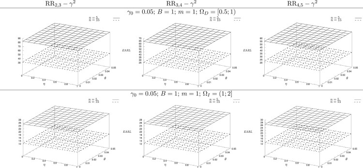
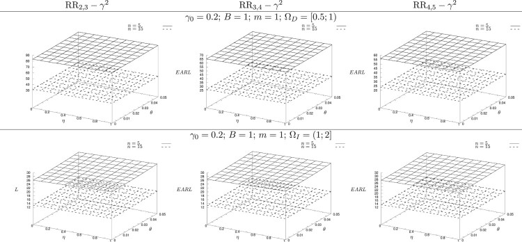
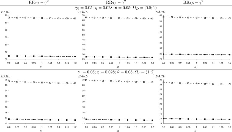
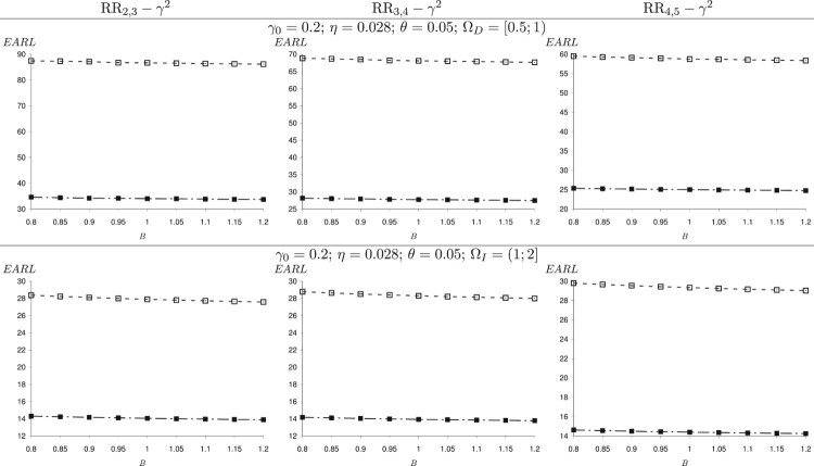
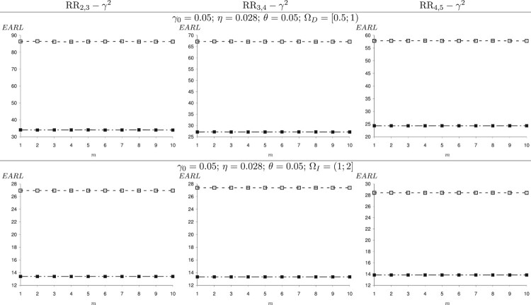
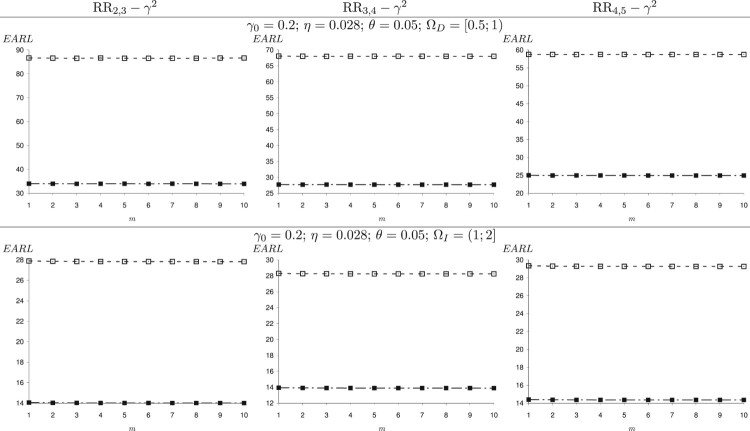
In the following simulation, we consider a specific range of decreasing shifts ${\mathrm{\Omega }}_D=[0.5,1)$ and increasing shifts ${\mathrm{\Omega }}_I=(1,2]$. Figures 2 and 3 show the change of EARL of the RR- ${\gamma }^2$ control charts when η varies in $[0,1]$ and θ varies in $[0,0.05]$ for ${\gamma }_0=0.05$ and ${\gamma }_0=0.2$, respectively. The slope of the plane which represents the EARL values from right to left and from outside to inside shows that the larger the values of η and θ, the larger the value of EARL. That is to say, these errors have negative effects on the performance of the RR- ${\gamma }^2$ charts. For example, in Figure 2 when n = 5, B = m = 1, and $\gamma =0.05$, we have EARL = 82.27 for $\theta =\eta =0$ (corresponding to no measurement errors), but $EARL=82.81$ for $\eta =0,\theta =0.05$ (corresponding to the negative effect of accuracy error), EARL = 83.42 for $\theta =0,\eta =0.3$ (corresponding to the negative effect of precision error), and EARL = 84.49 for $\theta =0.05,\eta =0.5$ (corresponding to the negative effect of both precision and accuracy error). The effect of B and m on the EARL is displayed in Figures 4–7 for both ${\gamma }_0=0.05$ and ${\gamma }_0=0.2$. We obtain a similar trend as the case of the specific shift size: When B increases, the EARL decreases and the EARL does not change significantly when m increases. The almost constant EARL line shows that the effect of m on these chart performance is insignificant. That is to say, increasing the value of m does not reduce the negative effect of measurement errors on the charts. In contrast, the plot of the EARL corresponding to n = 15 is always below the plot of the EARL corresponding to n = 5. That means, the sample size has a great impact on the RR ${}_{r,s}-{\gamma }^2$ charts' performance regardless of the measurement error.

Figure 2.

The effect of θ and η on the performance of the RR ${}_{r,s}-{\gamma }^2$ control charts in the presence of measurement errors for ${\gamma }_0=0.05$.

Figure 3.

The effect of θ and η on the performance of the RR ${}_{r,s}-{\gamma }^2$ control charts in the presence of measurement error for ${\gamma }_0=0.2$.

Figure 4.

The effect of B on the performance of the RR ${}_{r,s}-{\gamma }^2$ control charts in the presence of measurement errors for ${\gamma }_0=0.05$; n = 5 (-□-) and n = 15 ( $-◼-$).

Figure 5.

The effect of B on the performance of the RR ${}_{r,s}-{\gamma }^2$ control charts in the presence of measurement error for ${\gamma }_0=0.2$; n = 5 (-□-) and n = 15 ( $-◼-$).

Figure 6.

The effect of m on the performance of the RR ${}_{r,s}-{\gamma }^2$ control charts in the presence of measurement errors for ${\gamma }_0=0.05$; n = 5 (-□-) and n = 15 ( $-◼-$).

Figure 7.

The effect of m on the performance of the RR ${}_{r,s}-{\gamma }^2$ control charts in the presence of measurement error for ${\gamma }_0=0.2$; n = 5 (-□-) and n = 15 ( $-◼-$).

7. Illustrative example

In this section, we present an illustrative example of the implementation of the RR ${}_{r,s}-{\gamma }^2$ control charts in the presence of the measurement error. The real industrial data from a sintering process in an Italian company that manufactures sintered mechanical parts, which were introduced in [5], are considered.

The process manufactures parts guarantee a pressure test by dropping time $T_{pd}$ from 2 bar to 1.5 bar larger than 30 s as a quality characteristic related to the pore shrinkage. Since the presence of a constant proportionality ${\sigma }_{pd}={\gamma }_{pd}\times {\mu }_{pd}$ between the standard deviation of the pressure drop time and its mean had been demonstrated by the preliminary regression study relating $T_{pd}$ to the quantity $Q_C$ of molten copper, the quality practitioners decide to monitor the CV ${\gamma }_{pd}={\sigma }_{pd}/{\mu }_{pd}$ to detect changes in the process variability. According to the description in [5], an estimate ${\hat{\gamma }}_0=0.417$ is calculated from a Phase I dataset based on a root mean square computation. Phase II data are reproduced in Table 8.

Table 8. Illustrative example of Phase II dataset.

i	${\overline{X}}_i^{\ast }$	$S_i^{\ast }$	$\hat{\gamma }$	${\hat{\gamma }}^{\ast 2}$
1	906.4	476.0	0.525	0.27563
2	805.1	493.9	0.614	0.37700
3	1187.2	1105.9	0.932	0.86862
4	663.4	304.8	0.459	0.21068
5	1012.1	367.4	0.363	0.13177
6	863.2	350.4	0.406	0.16484
7	1561.0	1562.2	1.058	1.11936
8	697.1	253.2	0.363	0.13177
9	1024.6	120.9	0.118	0.01392
10	355.3	235.2	0.662	0.43824
11	485.6	106.5	0.219	0.04796
12	1224.3	915.4	0.748	0.55950
13	1365.0	1051.6	0.770	0.59290
14	704.0	449.7	0.639	0.40832
15	1584.7	1050.8	0.663	0.43957
16	1130.0	680.6	0.602	0.36240
17	824.7	393.5	0.477	0.22753
18	921.2	391.6	0.425	0.18062
19	870.3	730.0	0.839	0.70392
20	1068.3	150.8	0.141	0.01988

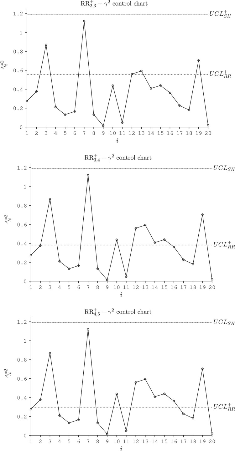
According to [19] under the presence of the measurement error, we suppose that the parameters of the linear covariate error model are $\eta =0.28$, $\theta =0.05$, B = 1, and m = 1. Based on the process engineer's experience, a specific shift size $\tau =1.25$ was expected to detect from the process. Therefore, we apply the upper-sided RR ${}_{r,s-{\gamma }^2}$ control chart to monitor the CV squared. The control limits of the RR ${}_{2,3}^{+}-{\gamma }^2$, RR ${}_{3,4}^{+}-{\gamma }^2$ and RR ${}_{4,5}-{\gamma }^2$ chart are found to be $UC{L}^{+}=0.5567$, $UC{L}^{+}=0.3821$ and $UC{L}^{+}=0.2972$, respectively. The values of ${\gamma }_i^{\ast 2}$ are then plotted in these charts (Figure 8) long with the control limit $UC{L}^{+}$. For the purpose of comparison, we also draw the control limit ( $UC{L}^{+}=1.1913$) of the original Shewhart control chart with the same parameters.

Figure 8.

The upward CUSUM- ${\gamma }^2$ control chart in the presence of the measurement error corresponding to the Phase II data in Table 8.

As can be seen from the Figure 8, the RR ${}_{2,3}^{+}-{\gamma }^2$, RR ${}_{3,4}^{+}-{\gamma }^2$ and RR ${}_{4,5}-{\gamma }^2$ chart signal the occurrence of the out-of-control condition by two-out-of-three, three-out-of-four, and four-out-of-five (respectively) successive plotting points above the corresponding control limits from the sample #12. Meanwhile, the Shewhart chart fails to detect this out-of-control condition.

8. Concluding remarks

In this paper, the performance of Run Rules control charts is improved slightly by monitoring the CV squared with the two one-sided charts rather than monitoring directly the CV with a two-sided chart as in a previous study in the literature. The effect of measurement errors on the performance of the RR ${}_{r,s}-{\gamma }^2$ control charts using a linear covariate error model is also investigated. We have pointed out the negative effect of measurement errors on the proposed charts: the increase of η and θ leads to an increase of EARL. Moreover, the obtained results show that measuring repeatedly is not an efficient method for limiting these unexpected effects. Extension to Run Rules EWMA and Run Rules CUSUM ${\gamma }^2$ type charts and the effect of the parameters estimation on their statistical properties are suggested as further important topics of research.

Funding Statement

Research activities of Phuong Hanh Tran have been funded by Vietnam International Education Development [Project 911].

Disclosure statement

No potential conflict of interest was reported by the author(s).

References

- 1.Breunig R., An almost unbiased estimator of the coefficient of variation, Econ. Lett. 70 (2001), pp. 15–19. doi: 10.1016/S0165-1765(00)00351-7 [DOI] [Google Scholar]
- 2.Castagliola P., Achoure A., Taleb H., Celano G., and Psarakis S., Monitoring the coefficient of variation using control charts with run rules, Qual. Technol. Quant. Manag. 10 (2013), pp. 75–94. doi: 10.1080/16843703.2013.11673309 [DOI] [Google Scholar]
- 3.Castagliola P., Achouri A., Taleb H., Celano G., and Psarakis S., Monitoring the coefficient of variation using a variable sampling interval control chart, Qual. Reliab. Eng. Int. 29 (2013), pp. 1135–1149. doi: 10.1002/qre.1465 [DOI] [Google Scholar]
- 4.Castagliola P., Achouri A., Taleb H., Celano G., and Psarakis S., Monitoring the coefficient of variation using a variable sample size control chart, Int. J. Adv. Manuf. Technol. 80 (2015), pp. 1561–1576. doi: 10.1007/s00170-015-6985-6 [DOI] [Google Scholar]
- 5.Castagliola P., Celano G., and Psarakis S., Monitoring the coefficient of variation using EWMA charts, J. Qual. Technol. 43 (2011), pp. 249–265. doi: 10.1080/00224065.2011.11917861 [DOI] [Google Scholar]
- 6.Manual , Measurement System Analysis, 4th ed., Automotive Industry Action Group, Southfield, 2010. [Google Scholar]
- 7.Kadri F., Harrou F., Chaabane S., Sun Y., and Tahon C., Seasonal ARMA-based SPC charts for anomaly detection: application to emergency department systems, Neurocomputing 173 (2016), pp. 2102–2114. doi: 10.1016/j.neucom.2015.10.009 [DOI] [Google Scholar]
- 8.Khaw K.W., Khoo M.B.C., Yeong W.C., and Wu Z., Monitoring the coefficient of variation using a variable sample size and sampling interval control chart, Comm. Statist. Simulation Comput. 46 (2017), pp. 5722–5794. doi: 10.1080/03610918.2016.1177074 [DOI] [Google Scholar]
- 9.Linna K.W. and Woodall W.H., Effect of measurement error on Shewhart control charts, J. Qual. Technol. 33 (2001), pp. 213–222. doi: 10.1080/00224065.2001.11980068 [DOI] [Google Scholar]
- 10.Muhammada A.N.B., Yeong W., Chonga Z., Limc S., and Khood M.B.C., Monitoring the coefcient of variation using a variable sample size EWMA chart, Comput. Ind. Eng. 126 (2018), pp. 378–398. doi: 10.1016/j.cie.2018.09.045 [DOI] [Google Scholar]
- 11.Nguyen H.D., Nguyen Q.T., Tran K.P., and Ho D.P., On the performance of VSI shewhart control chart for monitoring the coefficient of variation in the presence of measurement errors, Int. J. Adv. Manuf. Technol. 104 (2019), pp. 211–243. doi: 10.1007/s00170-019-03352-7 [DOI] [Google Scholar]
- 12.Noor-ul Amin M. and Riaz A., EWMA control chart for coefficient of variation using log-normal transformation under ranked set sampling, Iranian J. Sci. Technol, Trans. A: Sci. 44 (2020), pp. 155–165. doi: 10.1007/s40995-019-00805-2 [DOI] [Google Scholar]
- 13.Noor-ul Amin M., Tariq S., and Hanif M., Control charts for simultaneously monitoring of process mean and coefficient of variation with and without auxiliary information, Qual. Reliab. Eng. Int. 35 (2019), pp. 2639–2656. doi: 10.1002/qre.2546 [DOI] [Google Scholar]
- 14.Shongwe S.C., Malela-Majika J., and Castagliola P., A combined mixed-s-skip sampling strategy to reduce the effect of autocorrelation on the X-bar scheme with and without measurement errors, J. Appl. Stat. 5 (2020) pp. 1–25. doi: 10.1080/02664763.2020.1759033 [DOI] [PMC free article] [PubMed] [Google Scholar]
- 15.Tran K.P., Run rules median control charts for monitoring process mean in manufacturing, Qual. Reliab. Eng. Int. 33 (2017), pp. 2437–2450. doi: 10.1002/qre.2201 [DOI] [Google Scholar]
- 16.Tran K.P., Designing of run rules t control charts for monitoring changes in the process mean, Chemom. Intell. Lab. Syst. 174 (2018), pp. 85–93. doi: 10.1016/j.chemolab.2018.01.009 [DOI] [Google Scholar]
- 17.Tran K.P., Castagliola P., and Celano G., Monitoring the ratio of two normal variables using run rules type control charts, Int. J. Prod. Res. 54 (2016), pp. 1670–1688. doi: 10.1080/00207543.2015.1047982 [DOI] [Google Scholar]
- 18.Tran K.P., Du Nguyen H., Tran H., and Heuchenne C., On the performance of CUSUM control charts for monitoring the coefficient of variation with measurement errors, Int. J. Adv. Manuf. Technol. 104 (2019), pp. 1903–1917. doi: 10.1007/s00170-019-03987-6 [DOI] [Google Scholar]
- 19.Tran K.P., Heuchenne C., Balakrishnan N., and Khoo M.B.C., On the performance of coefficient of variation charts in the presence of measurement errors, Qual. Reliab. Eng. Int. (2018). [Google Scholar]
- 20.Tran P.H. and Tran K.P., The efficiency of CUSUM schemes for monitoring the coefficient of variation, Appl. Stoch. Models. Bus. Ind. 32 (2016), pp. 870–881. doi: 10.1002/asmb.2213 [DOI] [Google Scholar]
- 21.Tran P.H., Tran K.P., Truong T.H., Heuchenne C., Tran P.H., and Le T.M.H., Real Time Data-Driven Approaches for Credit Card Fraud Detection, Proceedings of the 2018 International Conference on E-Business and Applications, 2018, pp. 6–9.
- 22.Ye J., Feng P., Xu C., Ma Y., and Huang S., A novel approach for chatter online monitoring using coefficient of variation in machining process, Int. J. Adv. Manuf. Technol. 96 (2018), pp. 287–297. doi: 10.1007/s00170-017-1544-y [DOI] [Google Scholar]
- 23.Yeong W.C., Khoo M.B.C., Lim S.L., and Lee M.H., A direct procedure for monitoring the coefficient of variation using a variable sample size scheme, Comm. Statist. Simulation Comput. 46 (2017), pp. 4210–4225. doi: 10.1080/03610918.2015.1109659 [DOI] [Google Scholar]
- 24.Yeong W.C., Khoo M.B.C., Lim S.L., and Teoh W.L., The coefficient of variation chart with measurement error, Qual. Technol. Quant. Manag. 14 (2017), pp. 353–377. doi: 10.1080/16843703.2017.1304043 [DOI] [Google Scholar]
- 25.Zaidi F.S., Castagliola P., Tran K.P., and Khoo M.B.C., Performance of the hotelling T2 control chart for compositional data in the presence of measurement errors, J. Appl. Stat. 46 (2019), pp. 2583–2602. doi: 10.1080/02664763.2019.1605339 [DOI] [Google Scholar]
- 26.Zhang J., Li Z., Chen B., and Wang Z., A new exponentially weighted moving average control chart for monitoring the coefficient of variation, Comput. Ind. Eng. 78 (2014), pp. 205–212. doi: 10.1016/j.cie.2014.09.027 [DOI] [Google Scholar]
- 27.Zheng D., Li F., and Zhao T., Self-adaptive statistical process control for anomaly detection in time series, Expert. Syst. Appl. 57 (2016), pp. 324–336. doi: 10.1016/j.eswa.2016.03.029 [DOI] [Google Scholar]