ABSTRACT
Spatio-temporal disease mapping models give a great worth in epidemiology, especially in describing the pattern of disease incidence across geographical space and time. This paper analyses the spatial and temporal variability of dengue disease rates based on generalized linear mixed models. For spatio-temporal study, the models incorporate spatially correlated random effects as well as temporal effects. In this study, two different spatial random effects are applied and compared. The first model is based on Leroux spatial model, while the second model is based on the stochastic partial differential equation approach. For the temporal effects, both models follow an autoregressive model of first-order model. The models are fitted within a hierarchical Bayesian framework with integrated nested Laplace approximation methodology. The main objective of this study is to compare both spatio-temporal models in terms of their ability in representing the disease phenomenon. The models are applied to weekly dengue fever data in Peninsular Malaysia reported to the Ministry of Health Malaysia in the year 2017 according to the district level.
KEYWORDS: Disease mapping, Bayesian estimation, INLA, SPDE, dengue
1. Introduction
Dengue is the most ordinary mosquito-borne viral disease of humans, mainly transmitted by the female mosquitos Aedes aegypti and Aedes albopictus. Due to the dramatically increase of dengue cases day by day, dengue has become a major world-wide public health concern especially for regions near in tropical and sub-tropical climate and until now, many studies related to dengue are still ongoing with different approach and methodology. Presently, dengue outbreak can only be controlled using vector-controlled methods as licensed vaccine still in the developmental stage.
Mapping of disease risk has been recognized as an essential tool in the disease prevention and control strategies by investigating the spatial relationship of disease burden with the geographical distribution, environmental risk factors and human populations. Year by year, numerous methods for disease mapping have been expanded in accordance with the growing amount of routinely collected health information worldwide.
The availability of the areal unit data that is recorded periodically led to the expansion of the spatio-temporal dengue mapping analysis from time to time. For every spatial temporal data, it is believed that there is autocorrelation between areal study units as well as between previous and subsequent times. Usually, the observation from geographically nearby units and temporally close time periods tends to have more similar values than areal units and time periods that are situated at a great distance. Spatial autocorrelation can arise because of the neighbourhood effects, where the behaviours of individuals in an areal unit are influenced by individuals in adjacent units, and grouping effects where groups of people with similar behaviours choose to live close together. Meanwhile, temporal autocorrelation may occur because the data relate to largely the same populations or same environmental factors in consecutive time periods.
Various models in spatio-temporal disease mapping have been discussed in the previous studies. Most of the models are based on conditional autoregressions (CAR) models with extension to Besag, York and Mollié (BYM) models. For instance, Bernardinelli et al. [3] proposed a linear time trend model with an additional linear and a differential time trend. Next, Assunção et al. [1] modified the study by applying second degree polynomial. Knorr-Held [9] focuses on the inclusion of space–time interactions using non-parametric time models by proposing four types of interactions together with four different prior distributions for the interactions. The model proposed by Knorr-Held [9] is very popular in the spatio-temporal study because the inclusion of spatio-temporal interactions gives meaningful interpretations. Ugarte et al. [24] compare the performance of six space–time disease mapping models by adopting the extension proposed by Bernardinelli et al. [3] and Knorr-Held [9]. In other study, Martínez-Beneito et al. [16] link spatio-temporal study with the autoregressive approach. Besides that, in different study, Cameletti et al. [6] implemented the stochastic partial differential equation (SPDE) approach proposed by Lindgren et al. [13] in order to employ the spatial and temporal effects for point-reference data in a hierarchical spatio-temporal model.
In spatio-temporal study, the smoothing technique is not relating to the use of information from spatial neighbours only, but the context is lengthened to borrowing temporal neighbours too. Information in time is shared in a similar manner as information is shared in space. Hence, risks are smoother and more reliable since the model is based on a greater amount of information. The spatio-temporal study is also very interesting to explore because this study is not yet in abundance as spatial model study.
Bayesian models have become a familiar approach for smoothing purposes, both empirical Bayes (EB) and fully Bayes (FB). Several studies such as Clayton and Kaldor [8], Marshall [15] and Lahiri and Maiti [11] used the EB method for smoothing in their disease mapping studies while Besag et al. [4], MacNab et al. [14], and Wakefield [25] applied the FB technique. However, with the aid of modern programming, FB is preferably being used to solve the posterior distribution especially in a complex model that requires many parameters to be estimated. Commonly, estimating parameter with FB in most studies will involve Markov chain Monte Carlo (MCMC) algorithm computation but this method requires a huge computation time and may cause major Monte Carlo errors especially for a big data set.
In order to circumvent this drawback, an alternative approximation method using integrated nested Laplace approximation (INLA) has been proposed by Rue et al. [19]. INLA is a powerful tool for Bayesian analysis as it provides precise parameter estimates in a shorter time and more practical to use in wide fields and complex models vary from the generalized linear mixed model (GLMM), spatial model and spatio-temporal areal data model (e.g. [20,23]). Besides that, INLA also works well with SPDE for spatial geostatistical data as well as spatio-temporal geostatistical data (e.g. [5,6,10]).
As dengue is an infectious disease, it is believed that people close to the infected area tend to get infected easily compared to people farther from the infected areas (known as spatial effect) and the number of cases temporally close tend to have more similar values (known as temporal effect). Hence, statistical models that incorporate these two effects in a single analysis would provide a better estimation of dengue relative risks. With a deep concern on dengue incidence in Malaysia and in line with government's effort to control this problem, statistically research on dengue with the inclusion of spatial and temporal trend is considered in this paper because it is believed that there is a relationship between geographical areas and time points on dengue risk. It is hoped that this research may help the target audiences in planning more systematic vector-control prevention programmes especially for hotspots areas and also areas that have a tendency to become hotspots area. The objectives of this paper are to analyse the dengue disease phenomenon in Peninsular Malaysia through two different spatio-temporal models and to visualize the disease phenomenon using graphical representation. This study used areal data on weekly dengue incidence in 86 districts and 52 weeks in Peninsular Malaysia for the year 2017 that was obtained from Vector Borne Disease Sector, Ministry of Health Malaysia.
2. Methodology
Two models with different approaches are considered in this paper for comparison purpose. The first spatio-temporal model is based on Leroux spatial random effect proposed by Leroux et al. [12], while the second model is based on the SPDE approach proposed by Lindgren et al. [13]. For the temporal effect, an autoregressive model of first-order (AR1) model is defined for both models. These two models are built in the form of hierarchy and involve Gaussian Markov random fields (GMRF) model with the INLA for estimation.
2.1. Model I: spatio-temporal model with Leroux spatial random effect
Model I is built in the form of hierarchy with three stages, involving GLMM to estimate the relative risk estimation using several modifications of existing methods. GLMM allows modelling a wide range of response distributions such as Poisson distribution and allows inclusion of both fixed and random effects. The spatio-temporal hierarchical model is described in Table 2. The first stage of the hierarchy is the observational model. The study region, Peninsular Malaysia is divided into n areas as this study is focused on district level. Data for each area, i with time points, t are available for analysis. Assuming the number of dengue cases, conditional to the relative risk, to have Poisson distribution with mean, ,
where is an expected number of cases in district i for time t.
Taking logarithm to the both side of the mean, leads to
| (1) |
Different models are defined depending on the specification of the log risk, . In this paper, the log risk is modelled as
| (2) |
where α is the logarithm of the global risk, is referring to spatial random effect, is defined as the unstructured temporal random effect that accounts for temporal heterogeneity, is structured temporal random effect that allows for temporal dependence, and is space–time interaction random effect. This is a separable space and time model, where the spatial and temporal effects are joined separably. The advantage of this approach is in terms of computational cost. This approach is more practical and gives less computational burden compared to the non-separable model. According to Shaddick and Zidek [21], modelling the entire spatial-temporal structure jointly is often complex and impractical due to high dimensionality in most applications.
The second stage consists of the random effects in Equation (9) that can be modelled as GMRF as follows:
where this notation− denotes the Moore–Penrose generalized inverse of a matrix, and are the variance components corresponding to the spatial, temporal and spatio-temporal, is a spatial smoothing parameter varies between 0 and 1, is an identity matrix, is a identity matrix, is the spatial neighbourhood matrix, is the structure matrix of AR1. Here, the Leroux et al. [12] prior is considered for the spatial effect, and AR1 prior is considered for the temporal effects. Leroux prior is chosen as it can represent a range of weak and strong spatial correlation structures, while AR1 prior is chosen as it can estimate the temporal correlation naturally from the data. For the Leroux model, when , there is no spatial variability and the model reduces to independent model, . When , there is full spatial variability and the spatial model results to intrinsic autoregressive model, . is the structure matrix of space–time interaction. Briefly, GMRF is latent Gaussian model with conditional independence property and plays a predominant role in hierarchical model [18].
The entries of matrix follow the following rules:
where the diagonal elements are equal to (i.e. the number of neighbours of district i), and the off-diagonal elements are equal to for every district that adjacent to district i. Meanwhile, the structure for is in the following form:
where ρ is a temporal correlation and .
The space–time interaction structure matrix is given by the Kronecker product, corresponds to the structure matrices of the main effects. Similar to Knorr-Held [9], four different types of space–time interactions are considered and can be interpreted in a different way (refer Table 1).
Table 1. Four different types of space–time interaction terms.
| Space–time | |||
|---|---|---|---|
| interaction | Rank of | Description | |
| Type I | All are independent as they do not | ||
| have any structure in space and time | |||
| Type II | Each has a specific time trend but | ||
| independent to all other areas | |||
| Type III | Each has a specific spatial pattern | ||
| but no obvious temporal structure | |||
| Type IV | All are completely dependent over | ||
| space and time |
Note: Table followed Ugarte et al. [23].
Table 2. Summary of the Bayesian hierarchical model.
| Stages | Description |
|---|---|
| First stage | – The observational model, |
| – y is the observations | |
| Second stage | – Components in Equation (9), model as Gaussian Markov random fields (GMRF) with precision matrix Q, i.e. inverse covariance matrix, |
| – | |
| Third stage | – Hyperparameters, |
| – |
Maintaining the main effects and dropping the space–time interaction effect leads to the additive model. The additive model will be represented by Model 1. For the next models, models with different interaction types are run. Model 2, 3, 4 and 5 follow Type I, II, III and IV interactions respectively with the unstructured and the structured time effects. In addition, models without the unstructured time effects are considered in which Model 6 represents the additive models, Model 7 and 8 represent Type II and IV interactions respectively. Generally, unstructured temporal effect accounts for temporal heterogeneity while structured temporal effect allows for temporal dependence.
Besides, to guarantee identifiability of the interaction term δ, specific sum-to-zero constraints have to be used except for Type I interaction model. The vector δ follows an intrinsic Gaussian Markov random field (IGMRF). An IGMRF is improper and its structure matrix, is not full rank. Its improper density is denoted by and can be written as
| (3) |
where is a linear constraint for δ, A is a matrix consists of eigenvectors which span the null space, and e is a vector of zeros. The number of required linear constraint is equivalent to the rank deficiency of .
Next, the hierarchical model is completed by the third stage that consists of hyperparameters. Hyperparameters control the random effects in stage two and an appropriate prior distribution is assigned to all the hyperparameters. The prior distribution represents the information that is available for the parameters of interest and may influence the results (i.e. posterior distributions) and hence, should be carefully considered and compared. Usually, using the prior distributions based on a literature review to determine the prior distributions is helpful in Bayesian models. For details, see papers by Bernardinelli et al. [2] and Wakefield [25]. The only priors that should be specified correspond to the precision parameters are the inverse of the variance components; , , and . Here, the hyperprior distribution for the spatial components are and . For the temporal components, , and hyperprior are chosen. Meanwhile, a is used for the interaction component. For this study model, non-informative priors are used because there is a lack of information on the parameters in the study. This allows the data to speak for themselves and allows the posterior distribution to be dominated by likelihood or observed data.
Then, to estimate the marginal posterior distribution of all components in Equation (9), the method of approximation, INLA is used. In the INLA approach, the deviance information criterion (DIC) can be evaluated for the best model selection. According to Spiegelhalter et al. [22], DIC is the summation of the deviance posterior mean, and the effective parameters number, . The deviance posterior mean is a measure for model fit while the effective parameters number is a measure for model complexity. The best model is chosen based on the lowest DIC value. The lowest DIC value provides a balance between model fit and model complexity
| (4) |
2.2. Model II: spatio-Temporal model with SPDE for spatial random effect
The SPDE approach is based on some progressive tools of stochastic processes theory [13]. It is designed to use with geostatistical or point-referenced data and particularly for a continuous spatial process (i.e. a Gaussian Field) to estimate the spatial domain. Since this model is invented for point-referenced data, the centroids of every district are chosen as the actual locations of the dengue cases. This is in contrast with Model I where the spatial structure is based on area-level data.
SPDE involves a triangulation of the spatial domain, D defined as
| (5) |
where N is the total number of vertices of the triangulation, ψ is the set of basis functions and are Gaussian distributed weights. This consists in subdividing D into a set of non-intersecting triangles meeting at the edges. Figure 1 illustrates the concept of triangulation where the left panel shows the centroid of each district that acts as the locations of the dengue cases while the right panel lays a triangulation of the area with several vertices form based on the triangulation. The triangles are vary in size depending on how the mesh is specified. The mesh controls the number of vertices in the triangulation where the higher the number of mesh triangles, the finer the Gaussian Field (GF) approximation but the drawback is, the computational cost will be higher.
Figure 1.
Location of the 86 centroids of Peninsular Malaysia districts and the triangulation of Peninsular Malaysia region with more than 86 vertices.
Let represent the number of dengue case measured at centroid of location at week . The model equation is given by
| (6) |
where term refers to the error term and refers to the latent spatio-temporal process with changes in time following AR1 model,
| (7) |
where ρ is the AR1 temporal correlation coefficient and , is a zero-mean Gaussian field, assumed to be temporally independent by spatio-temporal covariance function as follows:
where is defined by the Matérn spatial covariance function and is given by
| (8) |
where h is the Euclidean spatial distance between two locations i and j, is the marginal variance, is the modified Bessel function of the second kind ν measures the degree of smoothness of the process and its value is fixed and greater than zero, κ is a scaling parameter related to the range r, where r corresponds to the distance where the spatial correlation is close to 0.1, for each ν, .
When the observations do not occur at mesh points, we need to construct an observation matrix called A matrix as a tool to map a field defined on the mesh to the observed locations. Hence, in short there are several steps involve in constructing SPDE model starting with creating a mesh, constructing A matrix, constructing SPDE model with Matérn spatial covariance function, organizing the data, making a formula and finally doing the inference.
For the SPDE model, the parameter vectors that need to be estimated are the standard deviation, the spatial range and also the autoregressive parameters for the spatial field, ρ. Similar to the previous model, the parameters involved in this study will be estimated through the INLA estimation method.
The details of INLA can be referred to Rue et al. [19], while the details of SPDE – INLA can be referred to Krainski et al. [10]. In this study, R-programming is used for the computational purpose with the aid of R-INLA package for both models.
3. Application to dengue disease case in peninsular Malaysia
3.1. Result and discussion for model I
The relative risk of dengue disease for each area in every time point is obtained from spatio-temporal model that has been described in Section 2. Table 3 shows the result for the eight fitted models that is based on a simplified Laplace approximation. The additive models exhibit the highest values of DIC and show the worst fit although their estimated model complexity is lower. This result implies the importance of including space–time interaction in the study model. Among the eight models proposed, Model 3 has the smallest DIC value. Hence, Model 3 is chosen as the best model in terms of model fit and complexity. This model consists of the spatial effect with a Leroux CAR prior, an unstructured temporal effect, a structured temporal effect with an AR1 prior and a Type II space–time interaction effect. Then after choosing the best model, this selective model has been refitted using the ‘full Laplace’ approximation and the result is used for relative risk computation.
Table 3. DIC values for the study models.
| Model | Space–time interaction | DIC | ||
|---|---|---|---|---|
| 1 | Additional model | 25,539.42 | 131.0821 | 25,670.5 |
| 2 | Type I | 17,317.59 | 1906.961 | 19,224.55 |
| 3 | Type II | 17,670.85 | 1041.567 | 18,712.42 |
| 4 | Type III | 18,201.65 | 1630.403 | 19,832.05 |
| 5 | Type IV | 18,297.99 | 962.1166 | 19,260.11 |
| 6 | Additional model | 25,540.45 | 129.215 | 25,669.67 |
| 7 | Type II | 17,680.31 | 1035.029 | 18,715.34 |
| 8 | Type IV | 18,291.68 | 965.9128 | 19,257.59 |
From Model 3, the estimated log-relative risks obtained can be separated into individual components: an overall global risk (), a risk related to the spatial location (), a temporal risk trend ( and ) common to all areas and an area-specific temporal risk trend () for each district. These are useful as the spatial and temporal effects can be varied across time and districts respectively.
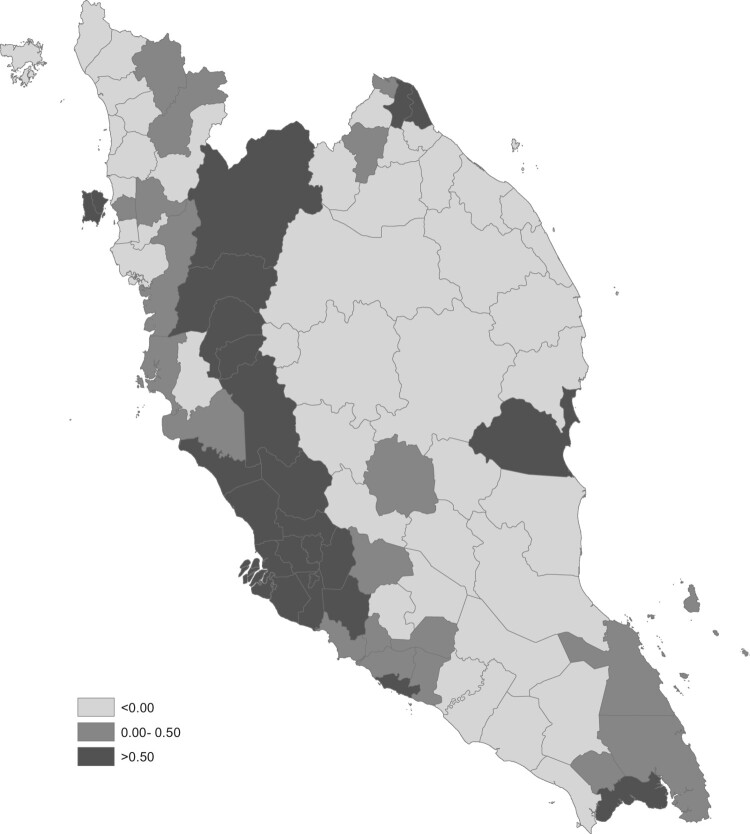
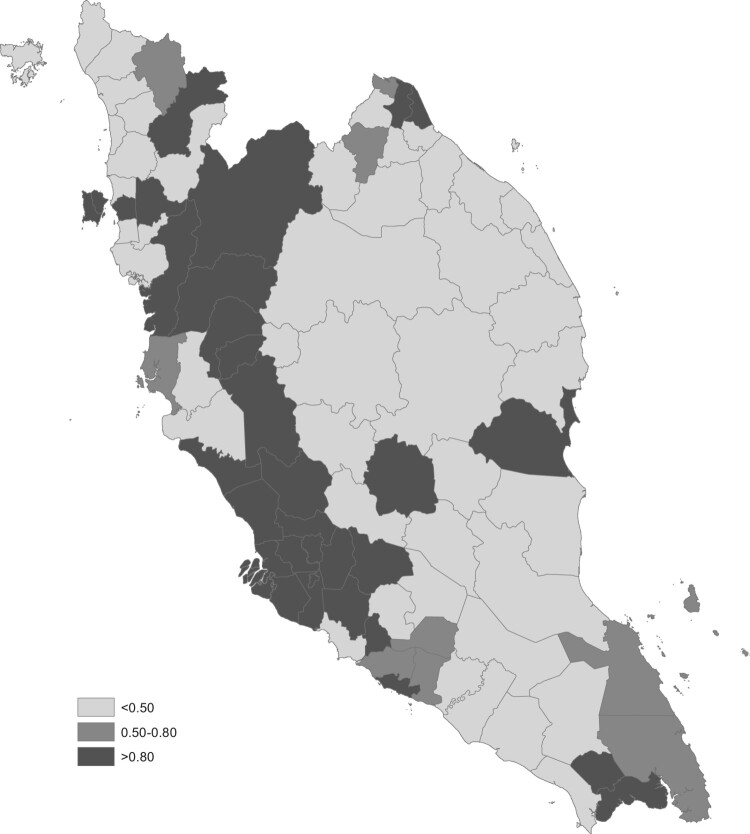
In disease mapping analysis, the results are normally presented in a map form to provide greater understanding of the trends and variability in spatio-temporal patterns. Figure 2 presents a spatial dengue risk, map associated to each district and constant throughout the year 2017. Meanwhile, Figure 3 presents the map of posterior probability that the spatial risk is greater than 1, . The degree of spatial risk is differentiated with different shades. For this model, the darker the region indicates the region's risk is higher. Mapping the probability that a relative risk is greater than a specified threshold of interest has been previously proposed by Clayton [7]. Usually, in the disease mapping studies, the regions with probabilities above 0.8 and 0.9 are considered as high risk regions, similar to Richardson et al. [17] suggested. In this study, a reference threshold equal to 1 and a cut-off value of 0.8 is used to detect high risk regions for all time periods. From both figures (Figures 2 and 3), it is clearly seen that the districts in west coast Peninsular Malaysia such as districts in Selangor, Kuala Lumpur, Penang, Perak, Melaka, Southern part of Johor, and some districts in Pahang are dengue high risk areas in the year 2017. Terengganu and Perlis demonstrate a good record in control over dengue threats as none of their districts lies in high risk region and moderate risk region. Meanwhile, Kuala Lumpur, Selangor and Perak show a bad and an alarming record as almost all districts in these states lie in high risk region category.
Figure 2.
The spatial pattern of dengue risk map, .
Figure 3.
The posterior probability of dengue risk map, .
Figure 4 presents the line graph of the general temporal trend of dengue risk common for all districts in Peninsular Malaysia. The temporal trend can be split into two components, AR1 component (represents by the joint line) and independent and identically distributed (i.i.d) component (represents by the dashed line). The line graph shows a non-linear trend with a fluctuating pattern throughout the year with slightly a decreasing pattern after week 33.
Figure 4.
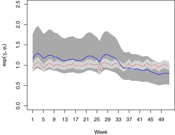
The general temporal trend of dengue risk.
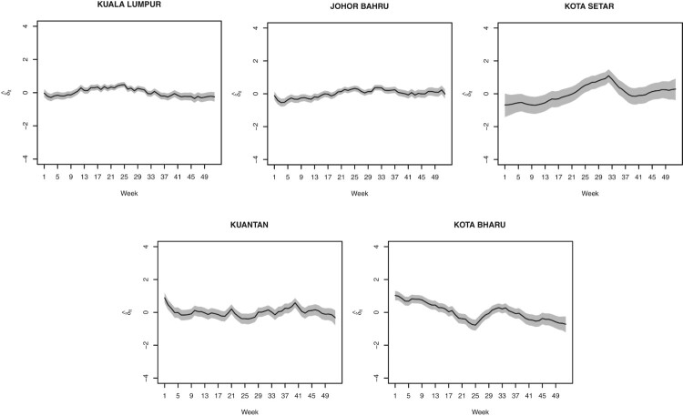
For the specific temporal trends, five selected districts are chosen for representing the northern, eastern, southern, western, and middle part of Peninsular Malaysia in order to observe the temporal trend of different districts. These specific temporal trends (in log scale) are represented in Figure 5. These line graphs are not converted to actual values because we are only interested to see their pattern as using the actual values will reveal the same pattern too. Johor Bahru, Kuantan and Kuala Lumpur show a steady pattern along the year. However, Kota Setar and Kota Bharu display a different trend. There is an increasing temporal trend for Kota Setar up to week 33 and decreasing before turning up at week 37. Meanwhile, for Kota Bharu, the time effect is decreasing at first 25 weeks and again after week 33.
Figure 5.
Specific temporal trends (in log scale) for five selected districts: Kuala Lumpur, Johor Bahru, Kota Setar, Kuantan and Kota Bharu.
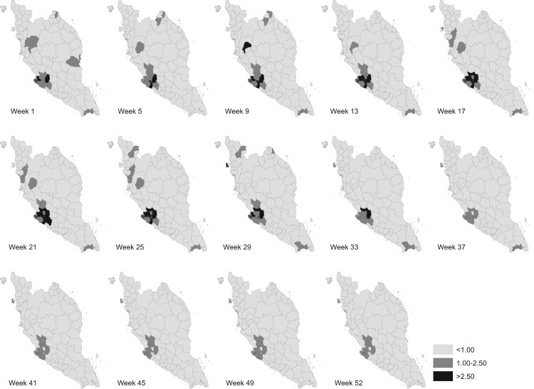
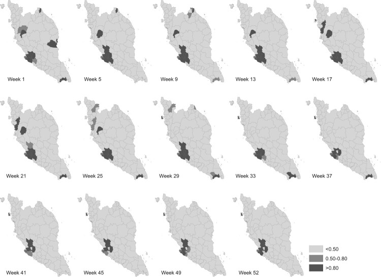
Figures 6 and 7 display several maps of the relative risk of dengue and the posterior probabilities that the relative risk greater than 1, for each district in Peninsular Malaysia from week 1 to week 52 of 2017 respectively. These figures give a clearer graphical representation in visualizing dengue disease phenomenon for all areas throughout the study period. Based on information from both figures, there are several districts that show a high significant risk of dengue disease in Peninsular Malaysia for the year 2017. A group of districts near to the most urbanized area in Peninsular Malaysia, Kuala Lumpur shows high significant risk throughout the week reported. However, for Kuala Lumpur, the relative risk of dengue is decreasing after week 33. This is different to Barat Daya in which the relative risk is increasing after week 33. Other than that, certain areas in Perak show a high relative risk in the first 25 weeks. For the east coast areas, only Kota Bharu reported a high relative risk and only for the first nine weeks. Meanwhile, the most southern district, Johor Bahru exhibits high dengue risk but does not show any significant trend.
Figure 6.
Relative dengue risk distribution.
Figure 7.
Posterior probability distribution, by districts.
Overall, it can be seen that the dengue trend is different for every district throughout the year. This is in line with Type II space–time interaction where there is a different temporal trend from region to region, but do not have any structure in space. Some regions experienced high dengue risk in a first half-year period, some regions started to have a high risk after the middle of the year, while some regions did not have any significant temporal trend. This can be related to different environmental factors for each district, for instance, climate factors, vector control schedule, urbanization and population density.
Districts that lie in a high risk category mostly are the districts that have a high population density among their states. A packed area facilitates the spread of the disease faster compared to an area with a less dense population.
In addition to the aforementioned result, a strong spatial dependence effect and a cluster of dengue risk seem to exist around Kuala Lumpur areas. Districts around Kuala Lumpur are the most densely populated areas in Peninsular Malaysia due to their location that located in and near to mother country. People chose to live there because of a wider job opportunity and a convenient accessibility.
However, further study on regression analysis and clustering analysis should be done to statistically confirm the factors that contribute to the elevation of dengue cases and the existence of clustering effect in this area.
3.2. Result and discussion for model II
SPDE model requires the exact points locations and also extra points that are obtained from the mesh construction. The centroid of each district is acted as the exact point locations with total number of points equal to 86. The dimension of A matrix based on the defined mesh is 4472 × 14,716. Dividing 14,716 with the number of time points reveals that the number of edges of the triangulation is equal to 283, implying there are 197 extra spatial points have been defined through the mesh construction. Table 4 shows the summary of the posterior marginal distributions for the likelihood precision and the random field parameters of SPDE models.
Table 4. The summary of the posterior marginal distributions for the likelihood precision and the random field parameters.
| Parameter for spatial field | Mean | Standard deviation | 95% Confidence interval |
|---|---|---|---|
| Standard deviation | 2.1636 | 0.1287 | (1.9264, 2.4319) |
| Range | 0.4684 | 0.0406 | (0.3926, 0.5525) |
| ρ | 0.9944 | 0.0007 | (0.9928, 0.9958) |
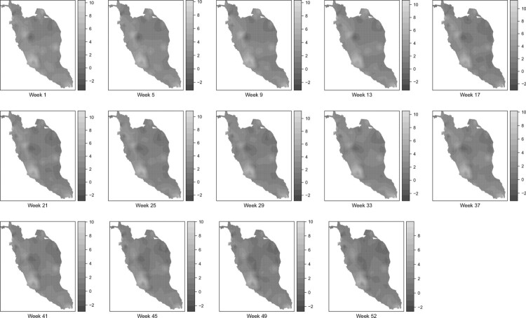
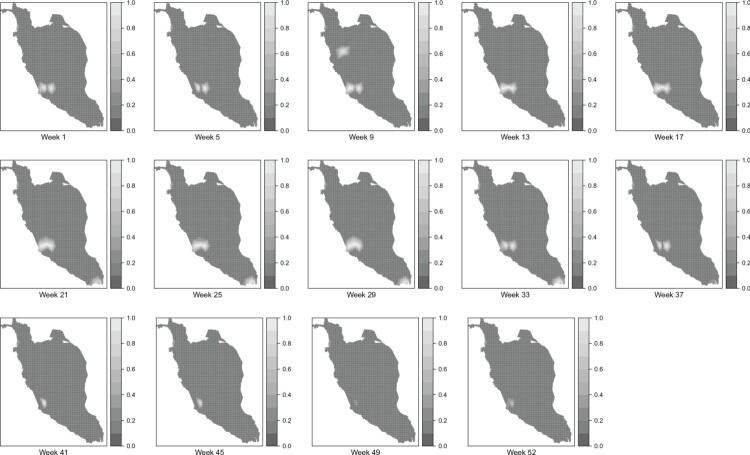
Meanwhile, Figures 8 and 9 display the map of the posterior mean of dengue disease cases and the map of the posterior probability of dengue disease cases exceeding the posterior mean of 10 respectively for the selected weeks in 2017 through the SPDE approach. These two figures are obtained from the posterior mean of the random field. The posterior exceedance probability map reported in Figure 9 can be used to detect the areas where the number of dengue cases is exceeding certain threshold depending on national regulations and hence, the focus should be given to those areas. Based on both figures, it can be seen that the areas located near to the most urbanized area, which is Kuala Lumpurare reported as the areas of high risk of dengue disease throughout the year. Besides that, areas located to the southern part of Perak and Johor also reported as areas with a high risk of dengue disease. Other areas that represent a high value of risk are areas in Penang, Kelantan and Pahang. In overall, it can be seen that both models present a similar result in mapping dengue disease. However, Model II visualizes the dengue disease phenomenon in Peninsular Malaysia without restricting to the district area. Hence, through the SPDE approach, several areas within the same district may have a different level of risk.
Figure 8.
Posterior mean of dengue disease cases for the selected weeks through the SPDE approach.
Figure 9.
Posterior probability of dengue disease exceeding posterior mean of 10 for the selected weeks through the SPDE approach.
4. Simulation study
Throughout this section, a simulation study is conducted to support the relative risk result that has been obtained in the previous section. A number of data sets are generated and for each of these data sets, estimation via INLA is performed. In simulation study for Model I, the simulated log relative risk is modelled as
| (9) |
and the number of cases is generated from a Poisson distribution with mean, . The random effects are generated from multivariate normal distributions as follows:
where and are model parameter estimates that have been obtained in the previous section. The estimated values are equal to the mean values of parameters in true values column in Table 5. Similar to the hyperparameters, the same set of hyperpriors that have been used in the previous section are considered for the simulation study. Table 5 displays the mean values and the standard errors of the estimated parameters as well as the 95% confidence interval of the estimated parameter for the true data and also the simulated data. Overall, the mean values of the estimated parameters for the simulated data are very close to the true values. The estimated values of all parameters for simulated data fall within the 95% confidence interval. Meanwhile for the standard errors, the simulated standard errors are reasonably well estimated.
Table 5. Mean values and standard errors of estimated parameters of INLA for Model I.
| True values | Simulated values | |||||
|---|---|---|---|---|---|---|
| Parameter | Mean | Standard error | 95% Confidence interval | Mean | Standard error | 95% Confidence interval |
| α | −1.3765 | 0.3364 | (−2.0594, −0.7094) | −1.3160 | 0.2777 | (−1.8612, −0.7714) |
| 1.8228 | 0.3487 | (1.2808, 2.6300) | 1.7162 | 0.3041 | (1.1872, 2.3699) | |
| 0.6823 | 0.1316 | (0.4051, 0.9029) | 0.6980 | 0.1244 | (0.4309, 0.9043) | |
| 0.0515 | 0.0526 | (0.0079, 0.1878) | 0.0513 | 0.0381 | (0.0145, 0.1500) | |
| 0.0046 | 0.0020 | (0.7141, 0.9916) | 0.0036 | 0.0014 | (0.8592, 0.9906) | |
| ρ | 0.9201 | 0.0748 | (0.0020, 0.0095) | 0.9468 | 0.0349 | (0.0017, 0.0070) |
| 0.0382 | 0.0030 | (0.0323, 0.0437) | 0.0134 | 0.0004 | (0.0127, 0.0141) | |
Next, the accuracy and the precision of INLA to estimate the relative risks of dengue disease have been evaluated by calculating the root mean squared error (RMSE) and the mean absolute error (MAE) of the estimated risks according to the following formula:
| (10) |
| (11) |
where denotes the estimated relative risk and B is the total number of simulated data sets. The result of the error measure is shown in Table 6. Based on the results, the error values obtained are small and it is reasonable to conclude that the INLA approach provides good point estimates in estimating relative risks of dengue disease in Peninsular Malaysia and Model I is working on similarly as structured data.
Table 6. The values of the RMSE and the MAE for the estimated risks.
| The accuracy and the precision measure | The error value |
|---|---|
| RMSE(r) | 0.0170 |
| MAE(r) | 0.0108 |
Meanwhile, for Model II, the mean values of the estimated parameters for the simulated data do not fall within the 95% confidence interval although their mean values are close to the true values. The result is displayed in Table 7.
Table 7. Mean values and standard errors of estimated parameters of INLA for Model II.
| True values | Simulated values | |||||
|---|---|---|---|---|---|---|
| Parameter for spatial field | Mean | Standard error | 95% Confidence interval | Mean | Standard error | 95% Confidence interval |
| Standard deviation | 2.1636 | 0.1287 | (1.9264, 2.4319) | 1.4386 | 0.0846 | (1.2793, 1.6120) |
| Range | 0.4684 | 0.0406 | (0.3926, 0.5525) | 0.7569 | 0.0699 | (0.6281, 0.9032) |
| ρ | 0.9944 | 0.0007 | (0.9928, 0.9958) | 0.9998 | 0.0000 | (0.9996, 0.9998) |
For the error measure, the result is displayed in Table 8. The error values obtained are small and reasonable although it is not as small as the error values in Table 6.
Table 8. The values of the RMSE and the MAE for the spatial field through the SPDE approach.
| The accuracy and the precision measure | The error value |
|---|---|
| RMSE(s) | 2.3578 |
| MAE(s) | 1.6966 |
Besides comparing the performance of these two models, based on these simulation results, it can also be concluded that INLA works well in estimating the parameter for both models under study. This is in line with previous studies that claimed INLA has been worked well in various models and problems.
5. Conclusion
There are several advantages and disadvantages of both models in comparison. Model I provides the result for overall spatial estimation, general and specific temporal trend as well as specific spatial pattern following the specific temporal trend for each area. Meanwhile, since the SPDE approach is based on continuous spatial random field, the result of Model II only provides the posterior mean of dengue disease incidence for the whole region in accordance to each time period. This is different to Model I, where we can separately analyse the spatial and temporal pattern of the disease under study such as what has been displayed in Figures 4 and 5.
For Model II, the advantage is that the evaluation of the spatial effect for every time point is no longer restricted to be similar to their districts, as the SPDE approach is based on mesh triangulation. Through the SPDE approach, researchers can analyse spatio-temporal model based on the exact location and obtained a more meaningful result. Besides that, the SPDE approach is a very interesting method for spatio-temporal study as it can be used for predicting spatio-temporal data in the locations and time points where the data are not been collected. It can also do continuous spatial estimation in continuous time points.
Based on this study, it can be concluded that both models are very beneficial for spatio-temporal study evolution. However, the appropriate model only can be chosen and determined by the nature of the data and also based on the objective of the research. In terms of computational time, the time taken to estimate parameter through the SPDE approach is slightly faster compared to the first model.
Besides that, our analysis of the dengue disease case in Peninsular Malaysia for the year 2017 from both models shows that the gap of the relative risks of dengue between the districts under study is big. There are areas that show significant high risk throughout the year such as areas near to the capital city of Malaysia, Kuala Lumpur which are Petaling, Sepang, Hulu Langat, Gombak, Klang and Hulu Selangor. Meanwhile, Barat Daya, Kinta and Johor Bahru have a tendency to become high dengue risk area. Hence, the authorities in charge should give prioritized to these areas in planning intervention strategies to reduce the dengue cases. Meanwhile, the other districts are still under control. However, precaution must be continued and monitoring should be done from time to time. Besides that, the results obtained also show that some areas have different temporal trends in dengue outbreak compare to other areas. Hence, the effective time for vector control activities for each district in Peninsular Malaysia can be identified. For example, districts such as Kota Bharu and some areas in Perak, the prevention control should be focused more on the beginning of the year, Barat Daya in the second term of the year while for districts in Selangor and Johor Bahru, the prevention should be done for the overall weeks throughout the year.
It can be also concluded that this study provides a useful starting point for spatio-temporal dengue analysis. The result in this study can be used in clustering analysis, hotspot identification and also spatial regression. As dengue is a major infectious disease in Malaysia and believes to have a strong relationship with environmental factors, adding covariate effects in the spatio-temporal model might give a more appropriate model for dengue study. This result is also advantageous in regional health planning, dengue disease surveillance and intervention, and also health funding allocation.
Acknowledgments
Special thanks to Vector Borne Disease Sector, Ministry of Health Malaysia for providing dengue disease data to this study.
Funding Statement
This research was financially supported by the Fundamental Research Grant Scheme (FRGS) offered by Ministry of Education Malaysia (203.PMATHS.6711666).
Disclosure statement
No potential conflict of interest was reported by the authors.
References
- 1.Assuncao R.M., Reis I.A. and Oliveira C.D.L., Diffusion and prediction of leishmaniasis in a large metropolitan area in Brazil with a Bayesian space–time model, Stat. Med. 20 (2001), pp. 2319–2335. doi: 10.1002/sim.844 [DOI] [PubMed] [Google Scholar]
- 2.Bernardinelli L., Clayton D. and Montomoli C., Bayesian estimates of disease maps: How important are priors?, Stat. Med. 14 (1995), pp. 2411–2431. doi: 10.1002/sim.4780142111 [DOI] [PubMed] [Google Scholar]
- 3.Bernardinelli L., Clayton D., Pascutto C., Montomoli C., Ghislandi M. and Songini M., Bayesian analysis of space–time variation in disease risk, Stat. Med. 14 (1995), pp. 2433–2443. doi: 10.1002/sim.4780142112 [DOI] [PubMed] [Google Scholar]
- 4.Besag J., York J. and Mollié A., Bayesian image restoration, with two applications in spatial statistics, Ann. Inst. Stat. Math. 43 (1991), pp. 1–20. doi: 10.1007/BF00116466 [DOI] [Google Scholar]
- 5.Blangiardo M., Cameletti M., Baio G. and Rue H., Spatial and spatio-temporal models with r-inla, Spat. Spatiotemporal. Epidemiol. 4 (2013), pp. 33–49. doi: 10.1016/j.sste.2012.12.001 [DOI] [PubMed] [Google Scholar]
- 6.Cameletti M., Lindgren F., Simpson D. and Rue H., Spatio-temporal modeling of particulate matter concentration through the SPDE approach, AStA Adv. Statist. Anal. 97 (2013), pp. 109–131. doi: 10.1007/s10182-012-0196-3 [DOI] [Google Scholar]
- 7.Clayton D.G., Bayesian methods for mapping disease risk, Geogr. Environ. Epidemiol.: Methods Small-Area Stud. (1992), pp. 205–220. [Google Scholar]
- 8.Clayton D. and Kaldor J., Empirical Bayes estimates of age-standardized relative risks for use in disease mapping, Biometrics 43 (1987), pp. 671–681. doi: 10.2307/2532003 [DOI] [PubMed] [Google Scholar]
- 9.Knorr-Held L., Bayesian modelling of inseparable space–time variation in disease risk, Stat. Med. 19 (2000), pp. 2555–2567. doi: [DOI] [PubMed] [Google Scholar]
- 10.Krainski E.T., Gómez-Rubio V., Bakka H., Lenzi A., Castro-Camilo D., Simpson D., Lindgren F. and Rue H., Advanced Spatial Modeling with Stochastic Partial Differential Equations Using R and INLA, Chapman and Hall/CRC Press, Boca Raton, 2018. [Google Scholar]
- 11.Lahiri P. and Maiti T., Empirical Bayes estimation of relative risks in disease mapping, Calcutta Stat. Assoc. Bull. 53 (2002), pp. 213–224. doi: 10.1177/0008068320020304 [DOI] [Google Scholar]
- 12.Leroux B.G., Lei X. and Breslow N., Estimation of disease rates in small areas: A new mixed model for spatial dependence, in Statistical Models in Epidemiology, the Environment, and Clinical Trials. The IMA Volumes in Mathematics and its Applications Vol. 116, M.E. Halloran and D. Berry, eds., Springer, New York, 2000, pp. 179–191.
- 13.Lindgren F., Rue H. and Lindström J., An explicit link between Gaussian fields and Gaussian Markov random fields: The stochastic partial differential equation approach, J. R. Stat. Soc.: Ser. B (Stat. Methodol.) 73 (2011), pp. 423–498. doi: 10.1111/j.1467-9868.2011.00777.x [DOI] [Google Scholar]
- 14.MacNab Y.C., Farrell P.J., Gustafson P. and Wen S., Estimation in Bayesian disease mapping, Biometrics 60 (2004), pp. 865–873. doi: 10.1111/j.0006-341X.2004.00241.x [DOI] [PubMed] [Google Scholar]
- 15.Marshall R.J., Mapping disease and mortality rates using empirical Bayes estimators, Appl. Stat. 40 (1991), pp. 283–294. doi: 10.2307/2347593 [DOI] [PubMed] [Google Scholar]
- 16.Martínez-Beneito M.A., López-Quilez A. and Botella-Rocamora P., An autoregressive approach to spatio-temporal disease mapping, Stat. Med. 27 (2008), pp. 2874–2889. doi: 10.1002/sim.3103 [DOI] [PubMed] [Google Scholar]
- 17.Richardson S., Thomson A., Best N. and Elliott P., Interpreting posterior relative risk estimates in disease-mapping studies, Environ. Health Perspect. 112 (2004), pp. 1016. doi: 10.1289/ehp.6740 [DOI] [PMC free article] [PubMed] [Google Scholar]
- 18.Rue H. and Held L., Gaussian Markov Random Fields: Theory and Applications, Chapman and Hall/CRC Press, Boca Raton, 2005. [Google Scholar]
- 19.Rue H., Martino S. and Chopin N., Approximate Bayesian inference for latent Gaussian models by using integrated nested Laplace approximations, J. R. Stat. Soc.: Ser. B (Stat. Methodol.) 71 (2009), pp. 319–392. doi: 10.1111/j.1467-9868.2008.00700.x [DOI] [Google Scholar]
- 20.Schrödle B. and Held L., Spatio-temporal disease mapping using inla, Environmetrics 22 (2011), pp. 725–734. doi: 10.1002/env.1065 [DOI] [Google Scholar]
- 21.Shaddick G. and Zidek J.V., Spatio-temporal Methods in Environmental Epidemiology, Chapman and Hall/CRC Press, Boca Raton, 2015. [Google Scholar]
- 22.Spiegelhalter D.J., Best N.G., Carlin B.P. and Van Der Linde A., Bayesian measures of model complexity and fit, J. R. Stat. Soc.: Ser. B (Stat. Methodol.) 64 (2002), pp. 583–639. doi: 10.1111/1467-9868.00353 [DOI] [Google Scholar]
- 23.Ugarte M.D., Adin A., Goicoa T. and Militino A.F., On fitting spatio-temporal disease mapping models using approximate Bayesian inference, Stat. Methods Med. Res. 23 (2014), pp. 507–530. doi: 10.1177/0962280214527528 [DOI] [PubMed] [Google Scholar]
- 24.Ugarte M., Goicoa T., Ibanez B. and Militino A., Evaluating the performance of spatio-temporal Bayesian models in disease mapping, Environmetrics: Off. J. Int. Environmet. Soc. 20 (2009), pp. 647–665. doi: 10.1002/env.969 [DOI] [Google Scholar]
- 25.Wakefield J., Disease mapping and spatial regression with count data, Biostatistics 8 (2006), pp. 158–183. doi: 10.1093/biostatistics/kxl008 [DOI] [PubMed] [Google Scholar]


