Towards in vivo neural decoding

Abstract

Conventional spike sorting and motor intention decoding algorithms are mostly implemented on an external computing device, such as a personal computer. The innovation of high-resolution and high-density electrodes to record the brain’s activity at the single neuron level may eliminate the need for spike sorting altogether while potentially enabling in vivo neural decoding. This article explores the feasibility and efficient realization of in vivo decoding, with and without spike sorting. The efficiency of neural network-based models for reliable motor decoding is presented and the performance of candidate neural decoding schemes on sorted single-unit activity and unsorted multi-unit activity are evaluated. A programmable processor with a custom instruction set architecture, for the first time to the best of our knowledge, is designed and implemented for executing neural network operations in a standard 180-nm CMOS process. The processor’s layout is estimated to occupy 49 mm${}^2$ of silicon area and to dissipate 12 mW of power from a 1.8 V supply, which is within the tissue-safe operation of the brain.

Introduction

Patients suffering from various neurological disorders and amputations may lose their ability to control some of their normal bodily functions or to take care of themselves entirely. A brain–machine interface (BMI) creates a link between the brain’s neural activity and the control of an external assistive device by bypassing dysfunctional neural pathways. Invasive BMIs record neural signals directly from the motor cortex using brain-implanted electrodes. By understanding how brain activity relates to behavior, the encoded motor intentions in the recorded neural signals can potentially be decoded into meaningful control commands to restore a patients’ ability to interact with their surroundings, via improved communication or actuating an assistive device such as computers and prostheses.

Conventional acquisition systems employ multi-electrode arrays (MEAs), which allow simultaneous recording of hundreds of channels. The wireless transmission of a large amount of recorded data can impose high power consumption and long delays, which restricts real-time and in vivo operation of BMIs. For example, the data rate for a Utah Array [1] with 100 recording channels sampled at 20 kHz with a 10-bit resolution is 20 Mbps. For this transmission rate, an implantable chip requires several hours of continuous operation and a few hours for recharging the battery [2]. The commonly employed acquisition systems are unable to precisely place electrodes to individually record from a single neuron. Hence, each electrode records the neuronal activities of a region, where generally tens of neurons are present and thus, providing the acquisition of multi-unit activity (MUA). Moreover, the fixed geometry of the conventional MEAs, such as the Utah Array, constrains the populations of neurons that can be accessed. They are made from rigid metals or semiconductors, which can limit their application and longevity.

It has been shown that complex brain processes are reflected by the activity of large neural populations and that the study of a few neurons provide relatively limited information. Therefore, advances in BMI systems rely on the ability to record from large populations of neurons in the order of thousands. Recent high-density micro-electrode array (HD-MEA) technology developed by Neuralink [3] use flexible polymer probes to provide greater bio-compatibility and longevity, as well as an unprecedented high-bandwidth and spatio-temporal resolution for long-term intra-cellular neural recording. An array of up to 3072 electrodes can be implanted individually by a neurosurgical robot offering single-neuron (single unit) resolution. Neural recording MEAs with neuron-level precision open a fascinating opportunity to investigate how large cell populations encode sensory behavior and motor function. Biological neurons communicate by means of firing electric pulses, called action potentials (APs) or spikes. Neural activity is usually sparse, and since the firing rates of neurons, which is the number of spikes emitted by a neuron over a given time interval, rarely exceeds 10 Hz, the data transmission rate will be reduced drastically by detecting spikes on an implanted chip and only transmitting the spiking information. For example, employing a MEA with 100 channels sampling at 20 kHz with a resolution of 10 bits per sample, would require 20 Mbps for transmitting raw signals. If only spiking activity is transmitted, the data transmission rate can be reduced to only 2 to 3 kbps, assuming that each electrode records the activity of two to three neurons firing at an average rate of 10 Hz.

Researchers often require single-neuron activity for the study of how neurons are correlated with each other for specific stimulus or for decoding motor intentions. Since in a conventional extracellular recording an implanted electrode can record the neural activity of neurons from a distance of up to about 140 micrometers [4], the neural signal recorded by an electrode consists of the cumulative neural activities of multiple adjacent neurons and the neural activity of relatively far away neurons contaminated by noise and technical artifacts, such as electrode drift, tissue-electrode noise, and electronics noise. Neurons in a local area often fire spikes of similar shape and amplitude, however, relative to the distance of an electrode to a neuron, the shape of spike waveforms will differ for various neurons [5]. This key fact allows the spiking activity of individual neurons to be distinguished and separated through a process, called spike sorting [6], which may assist neural decoding for certain applications. Spike sorting is the process of grouping detected spikes into clusters based on the similarity of their shapes. The resulting clusters thus correspond to the spiking activity of different putative neurons. Transmitting detected spike waveform shapes, assuming a spike waveform is represented by only 48 samples and that the recording channel detects two to three neurons firing at a rate of 10 Hz, would require data rates between 960 Kbps and 1.44 Mbps. Increases in channel counts, spiking frequency, or the number of neurons in the vicinity of the electrode can raise this data rate dramatically. An alternative approach is to perform neural signal processing in vivo and only transmitting decoded neural activity directly to an external assistive device. Neural decoding aims to translate the neural activity of the brain into quantifiable commands for controlling or communicating with an external device. When decoding neural activity into a discrete set of commands, the output data rate of decoding can be given as $R_d=\frac{\lceil {log}_2(N_c)\rceil }{\mathrm{\Delta }t{N}_{\mathrm{\Delta }}}$, where $\lceil ·\rceil$ denotes the ceiling operator, $N_c$ denotes the number of discrete commands, $\mathrm{\Delta }t$ denotes the time bin size over which spikes are counted, and $N_{\mathrm{\Delta }}$ denotes the number of time bins collected prior to performing decoding. For example, simple cursor control can be decomposed into a discrete set of movements {left, right, up, down, none}. If detected spikes are binned every 10 ms and 10 bins are collected prior to decoding, the output data rate is $R_d=30$ bps. Controlling a prosthetic arm with multiple degrees of freedom (DOF) increases the data rate due to the numerical resolution of kinematic variables. The output data rate can be given as $R_d=\frac{V_b{N}_v}{\mathrm{\Delta }t{N}_{\mathrm{\Delta }}}$, where $V_b$ denotes the number of variables and $N_v$ denotes the total number of variables. For example, consider a robotic arm with seven DOF (i.e., $\alpha$, $\beta$, and $\gamma$ endpoint; x, y, and z angles; and grip velocity) with 8 bits of resolution per variable. If spikes are binned every 10 ms and 10 bins are collected prior to decoding, the output data rate is $R_d=560$ bps. Note that this is considerably less than that for transmitting raw data, spike events only, or spike waveform outputs [7]. Moreover, in vivo decoding decreases the time required to transmit data and the offline processing time. Minimizing the processing latency between biological signal generation and intended motor function is important. It has been shown that in non-human primate trials, a maximum latency of about 150 ms between signal generation and the robotic arm movement results in natural-looking and smooth motion [8].

In this article, we discuss the feasibility of realizing in vivo neural decoding with and without spike sorting. More specifically, in Sect. 2, we first discuss how much information is contained in the two alternative spike train analysis methods. Section 3 discusses the impact of spike sorting on decoding performance. The design and training of a temporal convolutional neural network decoder is presented. Section 4 presents the design and implementation of a programmable neural network-based decoding processor. Various challenges for realizing in vivo neural decoding are discussed. Section 5 makes some concluding remarks.

Estimating information in neural spike trains

Cortical neurons use spike trains to communicate with other neurons. The output spike train of each neuron is a stochastic function of its input signals from other neurons. Understanding what information is encoded in its output spike train and what information is discarded, as well as quantifying how much information a single neuron transfers (or loses) from the input it receives (i.e., a sensory stimuli) to the activity of neuron (i.e., the neural code), are important for efficient decoding of the brain activity.

It is generally assumed that all the information contained in the spike train can be represented by the spike times. The simplest representation of a neuron’s response can be given by its firing rate. In addition to the firing rate of neurons, the relative timing between spikes also encodes information, which may be useful for decoding. Rate coding and temporal coding are two techniques for quantifying the information encoded in a neural spike train [9, 10]. Rate coding implies that the firing rate of a neuron represents the information encoded in the spike train, while temporal coding implies that the information is not only based on the firing rate, but also the relative timing of spikes. Rate coding can be divided into two categories: neuron rate coding and population rate coding. Population or ensemble rate coding is a measure of the firing rate of an ensemble of neurons rather than individual neurons.

A visual representation of the two rate coding methods over a two second snippet of a neural spike train is shown in Fig. 1a and b. Figure 1a shows the grey boxes horizontally, which represents the firing rate over the time interval T as a temporal average. Figure 1b shows the grey boxes vertically, representing the firing rate as a spatial average over all neurons over a time window T. Neuron firing rates are computed by counting the number of spike events occurring during a time window T, while ensemble firing rates are computed by counting the number of spike events occurring across an ensemble of neurons during a time window T. Both measures are then normalized by T, which results in units of Hz. It has been shown that the ensemble rate coding more closely resembles the brain’s natural coding scheme, by which ensembles of neurons communicate their accumulated activity with other neural populations [11]. This can be considered as a spatial average of the neural activity, whereas the neuron firing rates represent a temporal average over a longer time.

Fig. 1.

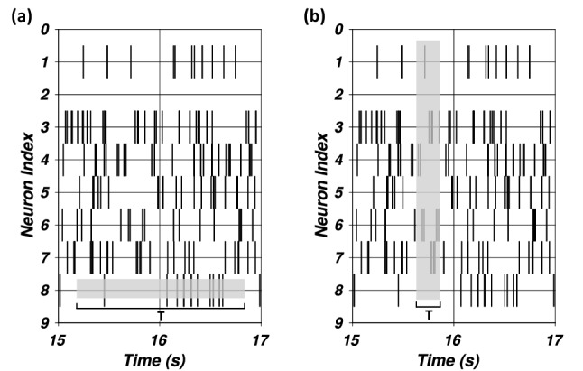
a Neuron rate coding and b ensemble rate coding

The entropy $S=-{\sum }_i[P_i{\log }_2{P}_i]$, where $P_i$ denotes the probability of a particular pattern of spike events, such as firing rate, denotes the average amount of “information” or “uncertainty” inherent to the random variable. Random variables with a more uniform distribution have a higher entropy, while distributions with a more localized peak have lower entropy. In other words, if a probability distribution is more biased toward specific outcomes, then there is less information encoded in the random variable compared to the one with higher entropy [12]. A coding scheme with a higher entropy can be interpreted as having a more uniform distribution and hence, a greater amount of information regarding the stimulus that caused the neural response.

For a spike train, we employ an estimation of entropy, in which the random variable is represented by the spike counts over small bins of $\mathrm{\Delta }\tau$ seconds over time windows of size T [13]. An intuitive interpretation of spike train entropy is that if a spike train is completely deterministic, it will have low variability in the time between spike events and by implication, its firing rates. This implies that a deterministic neuron encodes less information than a randomly firing neuron. To compare the entropy between the two rate coding schemes, we utilize the publicly available hc-2 dataset from the collaborative research on computational neuroscience [14]. The dataset consists of neural recordings from the CA1 region of the hippocampus of freely moving rodents over various experiments. The rodents were provided with water or food as a reward at random locations throughout a platform. For the recording session ec013.527, the entropy of the spike train and the calculated ensemble rate are given in Table 1. One can see that some neurons have low entropy, while others have relatively high entropy compared to the ensemble rate. The ensemble rate has a relatively high entropy and is not far from the mean entropy of all the neurons, (i.e., 33.93 bits/sec). Therefore, it can be assumed that using single unit firing rates would yield more information for decoding. In order to test this hypothesis, we divide the data into 125 ms intervals, which is equivalent to 5 samples of video frames to align the rodent positions to the physiology. A feed-forward neural network (FNN)-based decoder is trained to map firing rates (rate and ensemble coding) to rodent positions. The testing dataset contains 7797 samples, 80% of which are utilized for training, while the remaining 20% are used for validation and testing. Each sample in the dataset consists of binned neural data over 1.28 seconds with bins of size 25.6 ms, i.e., 50 time steps. The employed FNN has three hidden layers with tanh activation functions. The input dimension for the neuron-rate coding was 16, while the input dimension for the population-rate coding was one. The FNN was trained using the TensorFlow machine learning framework for Python for up to 1000 epochs, using early stopping to avoid overfitting to training data. The Adam optimizer with default parameters $lr=0.001$, ${\beta }_1=0.9$, ${\beta }_2=0.999$, and $ϵ=1\mathrm{e}-07$ was used for training. The input to the neural network was scaled (z-scored) as $x_z=(x-\tilde{x})/(x_{\sigma })$, where x denotes the training data and $\tilde{x}$ and $x_{\sigma }$ denote the mean and standard deviation of the training data, respectively, to have a zero-mean and unit variance distribution, which is useful for training. Additional statistical enhancements can be made by applying temporal smoothing of the input spike firing rates. One of the commonly employed methods is the Gaussian smoothing kernel [15], which convolves the input spike counts with a Gaussian curve of a pre-defined width. Applying Gaussian smoothing makes the distribution of the input data resemble a normal distribution more closely, which makes it easier to apply machine-learning algorithms to the data. The training dataset denotes the subset of the data used for optimizing the parameters of the network, while the validation dataset is used to assess the performance of the model during training. The testing dataset is used to evaluate the performance of the network, as it contains examples not observed during training.

Table 1.

The entropy rates for different neurons

Neuron index	Entropy rate (bits/sec)	Neuron index	Entropy rate (bits/sec)
1	18.17	10	17.12
2	10.97	11	27.01
3	45.41	12	42.98
4	44.92	13	41.01
5	33.32	14	35.41
6	30.96	15	42.83
7	35.51	16	43.68
8	34.69	Ensemble
9	38.94	Rate	38.25

Figure 2 shows the training and validation losses for the neuron and ensemble rate coding schemes. The testing loss for the neuron rate coding was 42.8 while the population rate loss was 43.29. The y-axis is plotted on a log scale to view the differences between the two rate coding schemes more easily. One can see that the neuron rate coding outperforms the ensemble rate decoding slightly due to the higher entropy for certain neurons and also due to the higher dimensional space to learn from compared to the single dimensional input of the ensemble rate coding scheme. Thus, we conclude that in the context of neural decoding, neuron-rate coding may outperform the population-rate coding.

Fig. 2.

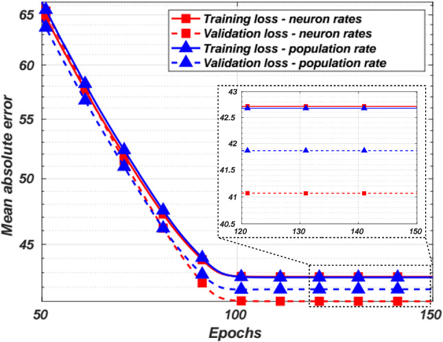
The training and validation loss for neuron rate coding and ensemble rate coding over various training epochs

Neural decoding and spike sorting

Investigating sorted and unsorted decoding paradigms

Spike sorting has been employed to extract the activity of individual single units influencing an electrode from the recorded MUA. Conventionally, spike sorting consists of several processing steps. First, spikes are detected from the background noise. Common detection techniques involve estimating the noise in the recorded and filtered signal and comparing it with a threshold. From detected spike waveforms, specific features are then extracted. These extracted features are then clustered into distinct groups, in which similar features and thus, similar spikes, are grouped together. A commonly employed clustering algorithm is k-means clustering [16], in which the feature vectors are clustered into k distinct groups, indicating up to k different single units found in the neural recording.

A desirable approach toward in vivo decoding could be avoiding spike sorting altogether, thus reducing the amount of in vivo computation and/or wireless data transmission. Without spike sorting, all threshold crossings of the voltage waveform on an electrode are treated as firing from one putative neuron. While this approach ignores the kinematic information provided by individual neurons recorded on the same electrode, this loss of information can potentially be avoided due to the significant enhancement in the recording technologies at the single neuron level [3]. We thus explore two possible decoding paradigms: (i) unsorted decoding and (ii) sorted decoding, as shown in Fig. 3. First, spikes are detected from the neural signals recorded by an implanted MEA. The unsorted decoding paradigm will consider detected spikes from all neurons recorded by each of the electrodes to create a multi-unit spike train (MUST). The sorted decoding paradigm employs spike sorting to cluster the activities of individual neurons detected by the spike detection unit and create a single-unit spike train (SUST). The raster plots in Fig. 3 are created based on the detected spikes from each electrode and sorted spikes, respectively, where the x and y axes represent time and the spiking activity of different neurons, respectively. The spike train in the unsorted decoding paradigm shows the spikes detected on each of the N recording electrodes. The spike train in the sorted decoding paradigm shows the sorted spiking activity of M single units. The MUST or SUST is then passed to the decoding unit, which can employ a variety of decoding algorithms. Traditionally, the decoding models of interest are FNNs and recurrent neural networks (RNNs). RNNs can encode temporal information in their hidden layers [17] while FNNs cannot due to the lack of temporal memory. We propose to use the temporal convolutional network (TCN) [18]. The TCN, shown in Fig. 4a, encodes temporal information in the input sequence with dilated convolutions at deeper layers and thus spanning the entire input sequence. The distinct network architecture of the TCN addresses many of the limitations of RNNs with learning temporal features, as the TCN does not propagate gradients over time, but rather through convolutional layers. The output of the TCN is connected to a layer to linearly map TCN outputs to the rodent positions. The convolutions are causal, which means that the TCN is appropriate for real-time neural decoding.

Fig. 3.

The in vivo neural decoding paradigms

Fig. 4.

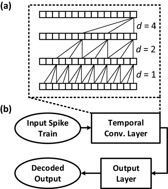
a The block diagram of a TCN layer and b the TCN-based decoder

Accurate spike sorting to retrieve the individual neuronal activities from multi-unit activity involves computationally- and memory-intensive algorithms and is often performed offline. Moreover, the requirement to sort spikes becomes more imposing with increasing the number of implanted recording electrodes, especially for spike sorting in vivo. Interestingly, some earlier work reported that decoding the spike detector’s outputs directly will make the system more robust for long-term use [19]. Also, several studies have suggested recently that spike sorting might not be critical for estimating intended movements in the motor BMI applications [20, 21]. In those ensemble decoding studies, the rate at which the filtered neural electrical signals crossed a pre-determined voltage threshold provided nearly an equivalent amount of information about the discrete direction of intended movements as did the spike rates of isolated, single neurons, irrespective of whether the threshold crossings detected on each electrode came from one or multiple neurons. Threshold crossing rates have successfully been used for real-time neural control in animals and humans, even years after the implantation of micro electrode arrays. Finally, the application of HD-MEA with neuron-level precision may eliminate the need for spike sorting altogether.

To study the effect of spike sorting on the performance of neural decoding, we utilize the publicly available hc-2 dataset [14]. The aim is to predict the location of the rodent based on the spiking activity of neurons in the hippocampus, which is the region of the brain responsible for cognitive processes related to spatial navigation and memory. For recording neural signals, four and eight channel tetrodes were used to improve spike sorting performance. The tip of each recording shank, which are the channels with the highest signal amplitude, were used for detecting spikes. A 32-sample waveform was created from each same-shank tetrode and hence, each spike is represented by an 8$\times$32 dimensional matrix. Dimensionality reduction was performed with discrete derivatives [22] to reduce the dimensionality to $8\times 3=24$ samples per waveform. k-means clustering was then performed to group feature vectors into 16 clusters, as done in [14].

Figure 5a shows the mean absolute error of the training of the unsorted and sorted TCN-based decoding paradigms using the training and validation sets over 100 training epochs. An important observation is that the sorted decoding paradigm has the advantage of a relatively faster convergence. However, as shown in Fig. 5b, both models converge to close $R^2$ scores for the validation set. Moreover, both paradigm perform well for the testing set, with the mean $R^2=0.9$ and $R^2=0.9$ for the sorted and unsorted paradigms, respectively. The unsorted paradigm reduces the dimension of the model’s input from the number of neurons to the number of recording shanks. While increasing the input’s dimension may increase the amount of information provided to the model, it has been shown that constraining the overall number of parameters in a model reduces overfitting [23]. We found that the TCN-based decoder offers robust decoding performance across a variety of spike detection algorithms, with the mean $R^2=0.97$ for both sorted and unsorted paradigms. Similarly, for this particular decoding task, it was found that a temporal sequence length of 75 time steps was optimal for time-series neural decoding with the mean $R^2=0.98$, compared to the feed-forward network with 50 time steps. Therefore, we employ the unsorted decoding paradigm for the real-time in vivo BMI realization.

Fig. 5.

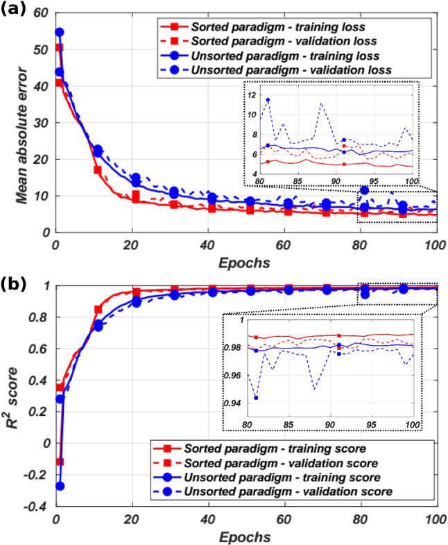
a The training performance and b the $R^2$ score of the TCN-based decoder for both decoding paradigms

Training and calibration

The training and calibration time of the neural decoder must be reasonable for a satisfying user experience. For example, it has been shown that for motor decoding applications, individual neurons often encode a preferred direction or movement [8]. Additionally, for single unit recordings, the same single units may not be present in the recorded neural signals across different sessions over multiple days or weeks. The process of re-training, or calibrating, neural network-based algorithms involves re-training a pre-trained model on a subset of the original training data in addition to the new data [24]. A common problem in network calibration, so called catastrophic forgetting [25], is that the model forgets data observations from earlier training sessions. In addition to retaining some of the previous data used for training, specific layers of the model may fix their weight values, similar to a transfer learning approach [26]. While the size of the updated training dataset or the total number of weight updates may be significantly smaller than the first training session, the time it takes to train the model remains relevant. A decoder for neural-controlled robotic arms reported in [27] has a calibration phase performed as follows. First, the subject is asked to carefully observe the automated movement of the arm for a given task. This is due to the modulation of neural firing patterns given the observation of the intended motion. The spike trains recorded during this process are then used to train the decoder. The observation-based decoder is then calibrated by allowing the subject to control the robotic arm with some amount of automated movement aid. The aid is intended to reinforce the subject to modulate their neural firing patterns that best correspond to the desired movement. Over several training sessions, the amount of automated movement aid is reduced and the subject learns to control the robotic arm on their own. The TCN-based decoder, for example, is better suited for real-time decoding and calibration due to the fact that there is no internal hidden state to compute over time. This allows TCNs to be trained significantly faster than RNN-based models of similar size. In our tests on a Desktop PC with an 8-core processor and 16 GB of RAM, we found that the TCN-based decoder took 25 min to train, while RNN models took over three hours to train. The training and calibration process could take longer if they are performed on a mobile device, which has considerably more processing limitations compared to a high-performance computer.

Towards an implantable decoding processor

While relatively small decoding architectures and algorithms can be employed for high levels of decoding performance, conventional BMIs still require an external device for processing neural signals. This imposes some major limitations: (i) for wireless BMIs, the amount and speed of data transfer are limited by the bandwidth of the communication medium; (ii) for wired BMIs, cables may limit the patient’s mobility and cause a poor user experience; (iii) the requirement of an external computing device means that the user must rely on additional devices for proper decoding operation. These limitations motivate the design and implementation of an in vivo machine learning-based decoding processor.

Figure 6a shows the conventional approach for wireless BMIs. Neural signals are recorded and processed by a spike count unit, which detects spikes from ambient noise and stores the spike count over a predefined amount of time before transmitting it to an external computing device. For example, the NeuraLink BMI transmits spike counts to a mobile device or a computer in 25 millisecond time bins for cursor control tasks [28]. Figure 6b shows the proposed approach for a fully-implantable wireless BMI. An in vivo processor would be able to directly process input spike trains and perform a variety of decoding tasks, such as controlling a prosthetic limb. An implantable processor is first programmed using a computer or mobile device. The processor is then able to interact directly with the external assistive device by performing neural decoding in vivo.

Fig. 6.

The system-level diagrams of a conventional and b the fully-implantable wireless BMIs

Due to the rapid advances in the field of machine learning, the processor would need to be programmable such that alternative decoding algorithms can be readily deployed using the same hardware. To this end, we have designed and implemented a custom neural network processor architecture for implementing arbitrary network operations. Our previously designed embedded processor architecture in [29] is enhanced to support arbitrary network operations, such as matrix multiplication, convolution, as well as the instructions required for implementing both feed-forward and temporal neural network architectures. The top-level datapath of the processor is shown in Fig. 7. The processor is a single-cycle reduced instruction-set computer (RISC) that executes an instruction over one clock cycle. Note that the relatively slow speed of biological signal generation and processing alleviates the need for high-speed and large-scale vector processing units that are typically found in conventional neural network accelerators. The designed processor has three memory units: the instruction memory Instr. Mem. used to store the program to execute; the register file Reg. File used to store program variables and memory addresses; and the data memory Data Mem., which is used to store neural network input data, weight parameters, and any necessary intermediate network computation results. The Instr. Mem. has a single address port that supports asynchronous read and synchronous write. The Reg. File is a dual-port memory unit with asynchronous read and synchronous write. The two outputs of the Reg. File, rf_rd1 and rf_rd2, are used to address the Data Mem., which is also a two-port memory unit with asynchronous read and synchronous write. Since the Data Mem. is addressed by values stored in the Reg. File, the write address of the Data Mem. is also addressed by rf_rd1. The computations of a decoding algorithm are performed in a sequential manner by the arithmetic logic unit ALU, which supports integer computations, as well as fixed-point operations. The ALU also has a dedicated activation function unit that implements the sigmoid, hyperbolic tangent (tanh), and rectified linear (ReLU) functions for hidden units of a neural network. The detailed implementation of the activation function unit is given in [29].

Fig. 7.

The top-level block diagram of the designed and implemented neural network processor

The instruction set for the designed neural network processor is given in Table 2. Each instruction is 29 bits long, with an instruction operation code (opcode) of 5 bits, and the remaining 24 bits are dedicated for defining register addresses or immediate values. For example, for the add_r instruction, three 8-bit fields denote the register source for the two ALU inputs as well as the write address to store the result in the register file. The instruction set consists of four types of instructions: integer computation, fixed-point computations, setup, and control instructions. The integer computations are mainly used to define program variables, such as loop counters. The fixed-point computations are used to perform neural network computations, such as matrix multiplication, element-wise addition/multiplication, and convolution. The fixed-point format consists of 16 bits for the integer part and 16 bits for the fractional part. Note that due to the relatively large amount of data required for neural networks, the Data Mem. is addressed by values stored within the register file. For example, the mult_e instruction performs the fixed-point multiplication of the value stored in the Data Mem. as indexed by the value stored in the register file at address $s1. For immediate instructions, the secondary input source to the ALU is either an 8-bit sign-extended immediate (SignExt[imm]) for integer computations, or a sign-extended and zero-padded 8-bit immediate, denoted as FPSignExt[imm]. The ALU has an internal accumulation unit that is enabled during fixed-point operations, which is useful for performing matrix multiplication, dot products, and convolutions. The setup instructions are used for miscellaneous operations, such as defining which activation function to use, swapping the order of ALU inputs, asserting the processor’s flag done, and reading values from Data Mem. to the processor’s output port. The control instructions are used for implementing loop constructs. Figure 8 shows the program snippet for computing the dilated convolution. This code segment is used iteratively for implementing the filter convolution operations.

Table 2.

The instruction set of the designed neural network processor

Instruction type	Instruction	Function
Integer computation	add_r $s1 $s2 $dst	RF[$dst] = RF[$s1] + RF[$s2]
	sub_r $s1 $s2 $dst	RF[$dst] = RF[$s1] - RF[$s2]
	mult_r $s1 $s2 $dst	RF[$dst] = RF[$s1] $\times$ RF[$s2]
	addi_r $s1 Simm $dst	RF[$dst] = RF[$s1] + SignExt[imm]
	subi_r $s1 Simm $dst	RF[$dst] = RF[$s1] - SignExt[imm]
	muli_r $s1 Simm $dst	RF[$dst] = RF[$s1] $\times$ SignExt[imm]
Fixed-point computation	add_e $s1 $s2	DM[$s1] + DM[$s2]
	sub_e $s1 $s2	DM[$s1] - DM[$s2]
	mult_e $s1 $s2	DM[$s1] $\times$ DM[$s2]
	addi_e $s1 $s2	DM[$s1] + FPSignExt[imm]
	subi_e $s1 $s2	DM[$s1] - FPSignExt[imm]
	muli_e $s1 $s2	DM[$s1] $\times$ FPSignExt[imm]
	wr_alu $s1	DM[$s1] = alu_result
	wr_acf1 $s1 $s2	DM[$s1] = DM[$s1] = ACF(alu_result, DM[$s2])
	wr_acf2 $s1 $s2	DM[$s1] = DM[$s1] = ACF(acc_result, DM[$s2])
	wr_acc $s1 $s2	DM[$s1] = DM[$s1] = acc_result
	rst_acc	Reset ALU accumulator to zero
Setup	iset_acf code	Set activation function to sigmoid, tanh, or ReLU
	sw_imm	Swap ALU inputs
	done	Assert processor done flag for 1 clock cycle
	rd_dm $s1	Read DM[$s1] and write to processor output port
Control	beq $s1 $s2 offset	Branch to PC+offset if RF[$s1] == RF[$s2]
	bneq $s1 $s2 offset	Branch to PC+offset if RF[$s1] != RF[$s2]
	jump jump_address	PC = jump_address
	jump_reg $s1	RA = PC+1; PC = RF[$s1]
	jump_return	PC = RA
	nop	No operation

Fig. 8.

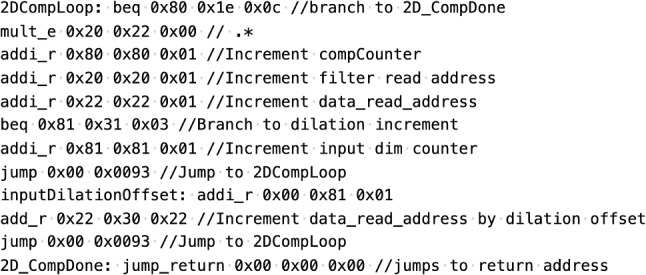
The program snippet for computing the dilated convolution

The synthesized ASIC layout of the designed neural network processor in a standard 180-nm CMOS process is shown in Fig. 9. Synthesis was performed with Synopsys Design Compiler, while place-and-route was performed with Cadence Innovus. The ASIC was synthesized with a maximum data memory depth of 4096 elements. The ASIC is estimated to occupy 49 mm${}^2$ of silicon area and consumes 12 mW of power while operating at 500 kHz. The power density of the ASIC is 24.4 $\frac{\mathrm{mW}}{{\mathrm{cm}}^2}$, which is within the tissue-safe limitation of about 40 $\frac{\mathrm{mW}}{{\mathrm{cm}}^2}$ [30]. The operating speed of the ASIC and the spike count bin size directly limit the size and complexity of models that can be implemented for real-time decoding. Consider the processor operating at f Hz, and the spike counts are accumulated over time bins of size $\mathrm{\Delta }t$ seconds. The number of clock cycles $\lambda$ for which to complete one time step of the real-time decoding can be given as $\lambda <\mathrm{\Delta }t\times f$. For example, given $\mathrm{\Delta }t=25$ ms, the model should complete computations within 12,500 clock cycles with an ASIC operating at 500 kHz. Table 3 gives an estimated number of clock cycles required for different types of network operations. As an example, consider that spike counts are generated for 96 input channels and the decoded output dimension is 2 (e.g., x and y coordinates of a computer cursor). For a TCN model with 3 layers, 8 filters per layer, and a temporal filter length of 3, the TCN requires 16,408 instructions. One can note that the constraint $\lambda <\mathrm{\Delta }t\times f$ may not be needed for non-continuous decoding schemes for which processing time is not vital. For example, if an output is only required after the entire temporal sequence is given, the processor can begin operating only when the final input spike counts are received. Alternatively, meeting the constraint for $\lambda$ will result in significantly faster inference time, as each temporal iteration of the decoder is computed immediately after the set of spike counts for the current time step is received.

Fig. 9.

The ASIC layout of the designed and implemented neural network processor

Table 3.

The estimated number of instructions for various network operations

Operation	Matrix 1 size	Matrix 2 size	Number of instructions
Matrix Mults.	$M_1\times N_1$	$N_1\times N_2$	$(M_1{N}_2)\times$
			$(3N_1+2)$
Convolutions	$M\times N$		$4(MN)+1$
Element-wise $+/-/\times$	$M\times N$		6MN

Conclusion

This article explored the feasibility of the in vivo neural decoding with and without employing spike sorting. It was found that the neuron-rate coding outperforms the population-rate coding, both in terms of the amount of entropy inherent to the coding scheme as well as the decoding performance. It was shown that the temporal convolutional network (TCN)-based decoder provides relatively accurate decoding while being trained and calibrated faster than alternative machine learning-based models. Moreover, it was also found that the TCN-based decoder provides robust decoding without the need for spike sorting, thus reducing the computational and memory requirements for the in vivo processing. The design and implementation of a programmable decoder processor with a custom instruction set architecture for executing neural network operations in a standard 180-nm CMOS process was presented. The ASIC layout was estimated to consume 49 mm${}^2$ of silicon area and to dissipate 12 mW of power from a 1.8 V supply, which is within the tissue-safe limitation of 40 mW/cm${}^2$.

Funding

This work was supported by the Center for Neurotechnology (CNT), a National Science Foundation (NSF) Engineering Research Center (EEC-1028725) and the NSF Award #2007131.

Declarations

Conflict of interest

The authors declare that they have no conflict of interest.

Ethical approval

This article does not contain any studies with human participants or animals performed by any of the authors.

References

- 1.Owens AL, Denison TJ, Versnel H, Rebbert M, Peckerar M, Shamma SA. Multi-electrode array for measuring evoked potentials from surface of ferret primary auditory cortex. J Neurosci Methods. 1995;58(1–2):209–220. doi: 10.1016/0165-0270(94)00178-J. [DOI] [PubMed] [Google Scholar]
- 2.Borton DA, Yin M, Aceros J, Nurmikko A. An implantable wireless neural interface for recording cortical circuit dynamics in moving primates. J Neural Eng. 2013;10(2):026010. doi: 10.1088/1741-2560/10/2/026010. [DOI] [PMC free article] [PubMed] [Google Scholar]
- 3.Musk E, et al. An integrated brain–machine interface platform with thousands of channels. J Med Internet Res. 2019;21(10):16194. doi: 10.2196/16194. [DOI] [PMC free article] [PubMed] [Google Scholar]
- 4.Buzsáki G. Large-scale recording of neuronal ensembles. Nat Neurosci. 2004;7(5):446–451. doi: 10.1038/nn1233. [DOI] [PubMed] [Google Scholar]
- 5.Gold C, Henze DA, Koch C, Buzsaki G. On the origin of the extracellular action potential waveform: a modeling study. J Neurophysiol. 2006;95(5):3113–3128. doi: 10.1152/jn.00979.2005. [DOI] [PubMed] [Google Scholar]
- 6.Lewicki MS. A review of methods for spike sorting: the detection and classification of neural action potentials. Netw Comput Neural Syst. 1998;9(4):R53. doi: 10.1088/0954-898X_9_4_001. [DOI] [PubMed] [Google Scholar]
- 7.Valencia D, Thies J, Alimohammad A. Frameworks for efficient brain–computer interfacing. IEEE Trans Biomed Circuits Syst. 2019;13(6):1714–1722. doi: 10.1109/TBCAS.2019.2947130. [DOI] [PubMed] [Google Scholar]
- 8.Velliste M, Perel S, Spalding MC, Whitford AS, Schwartz AB. Cortical control of a prosthetic arm for self-feeding. Nature. 2008;453(7198):1098–1101. doi: 10.1038/nature06996. [DOI] [PubMed] [Google Scholar]
- 9.Panzeri S, Schultz SR. A unified approach to the study of temporal, correlational, and rate coding. Neural Comput. 2001;13(6):1311–1349. doi: 10.1162/08997660152002870. [DOI] [PubMed] [Google Scholar]
- 10.Fetz EE. Temporal coding in neural populations? Science. 1997;278(5345):1901–1902. doi: 10.1126/science.278.5345.1901. [DOI] [PubMed] [Google Scholar]
- 11.Gerstner W, Kistler WM, Naud R, Paninski L. Neuronal dynamics: from single neurons to networks and models of cognition. Cambridge: Cambridge University Press; 2014. [Google Scholar]
- 12.Bishop CM, et al. Neural networks for pattern recognition. Oxford: Oxford University Press; 1995. [Google Scholar]
- 13.Strong SP, Koberle R, Van Steveninck RRDR, Bialek W. Entropy and information in neural spike trains. Phys Rev Lett. 1998;80(1):197. doi: 10.1103/PhysRevLett.80.197. [DOI] [Google Scholar]
- 14.Mizuseki K, Sirota A, Pastalkova E, Buzsáki G. Theta oscillations provide temporal windows for local circuit computation in the entorhinal-hippocampal loop. Neuron. 2009;64(2):267–280. doi: 10.1016/j.neuron.2009.08.037. [DOI] [PMC free article] [PubMed] [Google Scholar]
- 15.Chung MK. Gaussian kernel smoothing; 2020. arXiv preprint arXiv:2007.09539.
- 16.MacQueen J, et al. Some methods for classification and analysis of multivariate observations. Proceedings of the fifth Berkeley symposium on mathematical statistics and probability. 1967;1(14):281–297. [Google Scholar]
- 17.Elman JL. Finding structure in time. Cogn Sci. 1990;14(2):179–211. doi: 10.1207/s15516709cog1402_1. [DOI] [Google Scholar]
- 18.Lea C, Vidal R, Reiter A, Hager GD. Temporal convolutional networks: a unified approach to action segmentation. In: European Conference on Computer Vision. Springer; 2016. p. 47–54.
- 19.Kao JC, Stavisky SD, Sussillo D, Nuyujukian P, Shenoy KV. Information systems opportunities in brain–machine interface decoders. Proc IEEE. 2014;102(5):666–682. doi: 10.1109/JPROC.2014.2307357. [DOI] [Google Scholar]
- 20.Fraser GW, Chase SM, Whitford A, Schwartz AB. Control of a brain–computer interface without spike sorting. J Neural Eng. 2009;6(5):055004. doi: 10.1088/1741-2560/6/5/055004. [DOI] [PubMed] [Google Scholar]
- 21.Chestek CA, Gilja V, Nuyujukian P, Foster JD, Fan JM, Kaufman MT, Churchland MM, Rivera-Alvidrez Z, Cunningham JP, Ryu SI, et al. Long-term stability of neural prosthetic control signals from silicon cortical arrays in rhesus macaque motor cortex. J Neural Eng. 2011;8(4):045005. doi: 10.1088/1741-2560/8/4/045005. [DOI] [PMC free article] [PubMed] [Google Scholar]
- 22.Zamani M, Demosthenous A. Feature extraction using extrema sampling of discrete derivatives for spike sorting in implantable upper-limb neural prostheses. IEEE Trans Neural Syst Rehabil Eng. 2014;22(4):716–726. doi: 10.1109/TNSRE.2014.2309678. [DOI] [PubMed] [Google Scholar]
- 23.Zhang C, Bengio S, Hardt M, Recht B, Vinyals O. Understanding deep learning requires rethinking generalization; 2016. arXiv preprint arXiv:1611.03530.
- 24.Klabjan D, Zhu X. Neural network retraining for model serving; 2020. arXiv preprint arXiv:2004.14203.
- 25.Maltoni D, Lomonaco V. Continuous learning in single-incremental-task scenarios. Neural Netw. 2019;116:56–73. doi: 10.1016/j.neunet.2019.03.010. [DOI] [PubMed] [Google Scholar]
- 26.Torrey L, Shavlik J. Transfer learning. In: Handbook of research on machine learning applications and trends: algorithms, methods, and techniques. IGI global; 2010. p. 242–264.
- 27.Collinger JL, Wodlinger B, Downey JE, Wang W, Tyler-Kabara EC, Weber DJ, McMorland AJ, Velliste M, Boninger ML, Schwartz AB. High-performance neuroprosthetic control by an individual with tetraplegia. Lancet. 2013;381(9866):557–564. doi: 10.1016/S0140-6736(12)61816-9. [DOI] [PMC free article] [PubMed] [Google Scholar]
- 28.NeuraLink. Monkey MindPong. https://neuralink.com/blog/. 2021.
- 29.Valencia D, Fard SF, Alimohammad A. An artificial neural network processor with a custom instruction set architecture for embedded applications. IEEE Trans Circuits Syst I Regul Pap. 2020;67(12):5200–5210. doi: 10.1109/TCSI.2020.3003769. [DOI] [Google Scholar]
- 30.Wolf PD, Reichert W. Thermal considerations for the design of an implanted cortical brain–machine interface (bmi). Indwelling Neural Implants: Strategies for Contending with the In Vivo Environment; 2008. p. 33–8.