A novel traffic accident detection method with comprehensive traffic flow features extraction

Abstract

With the rapidly increasing of automobiles, traffic accidents are gradually becoming more frequent. This creates a great need for effective traffic anomaly detection algorithms. Existing methods shed light on directly inferring the abnormalities from traffic flow, which is short in features extraction and representation of traffic flows. In this paper, we propose three new traffic flow features, namely the road congestion, the traffic intensity, and the traffic state instability, for more comprehensive traffic status representation and anomaly detection. Residual analysis, quadratic discrimination, multi-resolution wavelet analysis are integrated for the extraction of the aforementioned features, which will be applied for the downstream tasks of traffic anomaly detection. Experimental results reveal that accident identification based on the proposed features is more effective than the raw traffic flow, which is supposed to provide an alternative approach for further applications and studies.

Introduction

In modern transport systems, various detectors provide actionable information in critical situations, which enable us to automatically discover the abnormality of the traffic stream in time. However, due to the complexity and variability in mass traffic behavior, it is difficult to directly identify abnormal traffic events from raw observed flow measures. Therefore, more sophisticated approaches that can extract features with clean meaning and effective representation are necessary for the automatic analysis of traffic flow data.

The detection of abnormal traffic accidents has already been realized based on machine learning algorithms, artificial intelligence [27] and deep learning [10]-related technologies. Xia [28] proposed an unsupervised method based on the sparse topic model to capture motion patterns and detect anomalies in traffic surveillance. Elizabeth Hou [12] addressed the problem of detecting anomalous activity in traffic networks where the network is not directly observed based on the Bayesian hierarchical model. Ronald D. Hagan [9] presented a case study on the analysis of New York City taxi traffic using the compound analytics framework. Silva Nuno [24] used PCA to analyze the attributes complexity of traffic features. Cuadra-Sanchez [4] focused on longitudinal traffic analysis, namely detecting sudden peak changes. Takahiro Kudo [14] detected traffic anomalies for every period of measured traffic via PCA. Youcef Djenouri [6] reviewed the use of outlier detection approaches in urban traffic analysis. Rupam Deb [5] presented a correlation-based imputation method to improve the quality of traffic flow. Shu-Bin Li [15] realized accident detection by taking into account the traffic ratio at the entrances and crossways. Seyed Hessam-Allah [11] provided a novel rule-based method to predict traffic accident severity according to user’s preferences.

Recently, Zheng Zhao [31] discussed a novel traffic forecast model based on long short-term memory (LSTM) network. Meanwhile, Mehrannia and BagiSiamese, et al [18] also investigate the deep representation of loop detector data using LSTM for automatic detection of freeway accidents. To deal with scenarios where only small datasets are available for training, Sabour and Rao, et al. [22] further develop the Siamese neural network-based DeepFlow to automatically analyze traffic flow data. Meanwhile, XGBoost [21], ensemble support vector machine [26], isolation forest [17], and other machine learning algorithms [23] are also applied for flow data-based abnormal traffic status detection.

In this study, we focus on the feature extraction of traffic flow data for more effective abnormal traffic events identification. Here the term abnormal traffic event refers to an exception point in time that the traffic system behaves abnormally and is significantly different from the previous normal behavior. This can be caused by natural factors (heavy rainfall in short-terms for example), or human factors such as traffic accidents. Fig. 1 shows the abnormal scene of vehicle collision. Since traffic flow parameters often show a significant trend under normal circumstances, the abnormal vehicle collision will cause a significant impact on traffic parameters [7] [20].

Fig. 1.

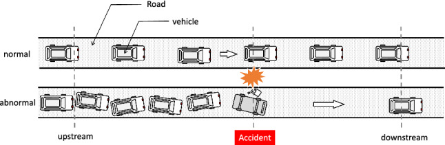
A visual statement of the vehicle collision accident, the normal condition (top) vs abnormal condition (bottom) after accident

However, the occurrence of traffic accidents is real-time, complex, and sporadic. Meanwhile, relationships between these accidents and their reflection on raw traffic flow parameters are hard to be summarized as clear rules. This brings great difficulties to automatic anomaly detection of traffic status. Based on the I80-E highway traffic flow data and accident records provided by the US PeMS system [30], we propose three new traffic flow features, namely the road congestion, the traffic intensity, and the traffic state instability, for more comprehensive traffic status representation and anomaly detection. Our study is executed according to the flowchart shown in Fig. 2.

Fig. 2.

Flowchart of traffic accident detection with the proposed feature extraction method

Methodology

Road congestion features

Road congestion refers to the traffic phenomenon caused by the traffic vehicle surge. McMaster algorithm is an algorithm based on the theoretical model of highway traffic [29] state catastrophe. However, during our application of the McMaster algorithm to the I80-E highway data, we find there are three limitations in the McMaster algorithm: (1) The critical values of occupancy and volume greatly depend on human analysis. (2) The parameter and configuration of different traffic detector/detectors are diverse, which needs us to analyze case-by-case. (3) The McMaster algorithm ignores the observed traffic parameters of speed. Meanwhile, it lacks consideration of other kinds of anomalies.

Therefore, we develop a new method to eliminate the above limitations. Fig. 3 demonstrates the traffic flow data of the detector S400430, where the X-axis represents the flow, Y-axis is the occupancy, and the color illustrates the speed. When the speed is faster than 50, the road is in the non-congestion state, and the flow is linear related to the occupancy. On the contrary, in the state of road congestion (speed is lower than 50), the flow and occupancy no longer satisfy the simple linear relationship, which forms several clusters away from the linear normal trends.

Fig. 3.

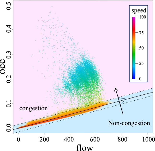
Scatter plot of the traffic flow data

According to the above characteristics of road congestion, we design road congestion identification features based on the Quadratic Discrimination Analysis (QDA) algorithm [3]. We utilize the following linear basis function model to map the flow $X_{\mathit{flow}}$ into the occupancy $X_{\mathit{occ}}$ for the non-congestion state:

$$\begin{array}{c}\hfill X_{\mathit{occ}}=a+b{X}_{\text{flow}}\end{array}$$ 1

where the constant a represents the vertical intercept, and b represents the slope of the linear basis function. Then, the residual $E_{\mathit{occ}}$ between the predicted occupancy $X_{\mathit{occ}}$ and the ground truth $X_{\mathit{occ}}^{\ast }$ is adopted to measure the state of from the:

$$\begin{array}{c}\hfill E_{\mathit{occ}}=X_{\mathit{occ}}^{\ast }-X_{\mathit{occ}}.\end{array}$$ 2

Then, the non-congestion occupancy of each point can be estimated by the linear relationship, while these observations are roughly labeled by the $3\sigma$ criterion [25] according to the residual difference with the real occupancy. Substituting each point flow $X_{\mathit{flow}}$ into the above linear relationship, it can be found that the $E_{\mathit{occ}}$ basically satisfies the Gaussian distribution with a mean of 0. Since the residual of the data points in the uncongested state is basically in the normal range, the residual value in the congestion state is obviously large. According to the $3\sigma$ criterion, the point of $E_{\mathit{occ}}>3\sigma$ can be considered to be in a road congestion state, where $\sigma$ is the standard deviation of $E_{\mathit{occ}}$. Finally, the Quadratic Discrimination Analysis (QDA) algorithm is used for supervised learning to predict congestion probability. The conclusion based on the $3\sigma$ criterion is only a rough discriminant conclusion, whether it is crowded or not. In order to obtain more accurate conclusions, the QDA algorithm [3] is used to obtain a classification prediction model. Applying the model to the detector data, the congestion probability of each point can be achieved, indicating the degree of road congestion.

Traffic intensity features

Traffic intensity refers to the number of vehicles detected by a detector per unit time. Since traffic patterns for working days and holidays are different, therefore, traffic data of Saturdays, Sundays, and legal holidays in the United States are marked for further analysis. Then, the short-term historical data of flow data are collected for the forecast of trend values in each day. The median of non-holiday traffic intensity in the first two weeks (about 10 days) is used as the trend values for working days. Meanwhile, the median of holidays traffic intensity in the first four weeks (about 8 days) is used as the trend values for holidays.

We take the following approach for the extraction of traffic intensity anomaly features. Firstly, the differences between actual and predicted occupancy and speed are calculated for each moment. Assuming that $X_{\mathit{occ}}$ and $X_{\mathit{speed}}$ represent actual data values of occupancy and speed at a certain time, respectively, while $T_{\mathit{occ}}$ and $T_{\mathit{speed}}$ indicate their corresponding predicted values. When there is no anomaly, $D_{\mathit{occ}}$ and $D_{\mathit{speed}}$ tend to 0. When abnormalities occur and traffic increases, $D_{\mathit{occ}}$ will be far greater than 0, and $D_{\mathit{speed}}$ will be far less than 0. In contrast, $D_{\mathit{occ}}$ will be far less than 0, and $D_{\mathit{speed}}$ will be far greater than 0 if traffic decreases.

Then, the cumulative probability density functions of $D_{\mathit{speed}}$ and $D_{\mathit{occ}}$ according to normal distribution are estimated. As can be observed in Fig. 4, we find that the empirical distribution of $D_{\mathit{occ}}$ and $D_{\mathit{speed}}$ of each detector is quite similar with the probability density curves of corresponding normal distribution. To further validate this observation, we performed the Kolmogorov–Smirnov normal likelihood test [16] for $D_{\mathit{occ}}$ and $D_{\mathit{speed}}$, while the testing results are presented in Table 1.

Fig. 4.

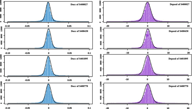
Histogram of $D_{\mathit{occ}}$ and $D_{\mathit{speed}}$ for partial detectors

Table 1.

Kolmogorov–Smirnov normality test result of D occ and D speed for partial detectors

Detector	The normal confidence coefficient of $D_{\mathit{occ}}$	The normal confidence coefficient of $D_{\mathit{speed}}$
S400027	0.656	0.683
S400430	0.772	0.705
S401895	0.719	0.715
S400770	0.703	0.658
S401195	0.801	0.794
S401892	0.693	0.644
S408632	0.614	0.696
S401269	0.678	0.712

It is confirmed that the distribution of $D_{\mathit{occ}}$ and $D_{\mathit{speed}}$ on each detector obey the normal distribution (with expectation 0 and statistic variances, respectively) with large confidence values. Therefore, the abnormal traffic intensity features $P_{\mathit{more}}$ and $P_{\mathit{less}}$ can be calculated from the cumulative probability function of approximated normal distributions. According to the definition of cumulative probability function of normal distribution, the cumulative probability density functions of $D_{\mathit{occ}}$ and $D_{\mathit{speed}}$ are:

$$\begin{array}{c}\hfill P_{\mathit{occ}}\left(D_{\mathit{occ}}\right)=\frac{1}{2}\left(1,+,\text{erf},\left(\frac{D_{\mathit{occ}}}{\sqrt{2}{\delta }_{\mathit{occ}}}\right)\right)\end{array}$$ 3

$$\begin{array}{c}\hfill P_{\text{speed}}\left(D_{\text{speed}}\right)=\frac{1}{2}\left(1,+,\text{erf},\left(\frac{D_{\text{speed}}}{\sqrt{2}{\delta }_{\text{speed}}}\right)\right)\end{array}$$ 4

where ${\delta }_{\mathit{occ}}^2$ and ${\delta }_{\mathit{speed}}^2$ are the statistic variances of $D_{\mathit{occ}}$ and $D_{\mathit{speed}}$, respectively. Then, the abnormal traffic intensity features $P_{\mathit{more}}$ and $P_{\mathit{less}}$ are defined as:

$$\begin{array}{c}\hfill P_{\text{anorm}}=P_{\text{occ}}\left(D_{\text{occ}}\right)\ast \left(1,-,P_{\text{speed}},\left(D_{\text{speed}}\right)\right)\end{array}$$ 5

$$\begin{array}{c}\hfill P_{\text{more}}=\left\{\begin{array}{cc}2.0\ast \left(P_{\text{anorm}},-,0.5\right);\hfill & P_{\text{anorm}}>0.5\hfill \\ 0.0;\hfill & P_{\text{anorm}}\le 0.5\hfill \end{array}\right)\end{array}$$ 6

$$\begin{array}{c}\hfill P_{\text{less}}=\left\{\begin{array}{cc}2.0\ast \left(0.5,-,P_{\text{anorm}}\right);\hfill & P_{\text{anorm}}\le 0.5\hfill \\ 0.0;\hfill & P_{\text{anorm}}>0.5\hfill \end{array}\right).\end{array}$$ 7

The value ranges of $P_{\mathit{more}}$ and $P_{\mathit{less}}$ are both (0,1). A high $P_{\mathit{more}}$ value indicates an abnormal increase in traffic intensity, while a higher $P_{\mathit{less}}$ indicates an abnormal decrease. Compared with directly using $D_{\mathit{occ}}$ and $D_{\mathit{speed}}$ for the abnormal traffic intensity representation, $P_{\mathit{more}}$ and $P_{\mathit{less}}$ effectively eliminate the magnitude differences of $D_{\mathit{occ}}$ and $D_{\mathit{speed}}$ among different detectors.

Traffic state instability features

We also develop a wavelet analysis-based approach to extract features for the representation of traffic state instability. This approach is applied to the series of three raw observed traffic parameters (flow, speed, and occupancy), and the corresponding local activity and fluctuation intensity features are obtained for the representation of overall and local variations of traffic flows.

The traffic state instability features are extracted based on the multi-resolution wavelet analysis framework. It is necessary to eliminate local fluctuations in the flow data that are independent of the overall trend changing. Therefore, we calculate the overall trend of traffic flow through a discrete binary wavelet transform [19]-based frequency domain smoothing algorithm. In our approach, the Daubechies wavelet basis is applied. According to Daubechies wavelet function $\psi (t)$ and scale function $\varphi (t)$:

$$\begin{array}{c}\hfill \left\{\begin{array}{c}{\psi }_{j,k}(t)=2^{-j/2}\psi \left(2^{-j},t,-,k\right)\hfill \\ {\varphi }_{j,k}(t)=2^{-j/2}\varphi \left(2^{-j},t,-,k\right)\hfill \end{array}\right).\end{array}$$ 8

Then, the trend $f_a^j(t)$ and detail $f_d^j(t)$ on the j-th scale can be constructed step by step:

$$\begin{array}{c}\hfill \left\{\begin{array}{c}{f}_a^j(t)={\sum }_k{c}_{j,k}{\varphi }_{j,k}(t);c_{j,k}=\int f(t)\overline{{\varphi }_{j,k}(t)}dt\hfill \\ f_d^j(t)={\sum }_k{d}_{j,k}{\psi }_{j,k}(t);d_{j,k}=\int f(t)\overline{{\psi }_{j,k}(t)}dt\hfill \end{array}\right)\end{array}$$ 9

In the above definition, $c_{j,k}$ is the scale expansion coefficient and $d_{j,k}$ is the wavelet expansion coefficient. Setting J as an arbitrary scale, traffic flow data can be reconstructed by:

$$\begin{array}{c}\hfill \mathrm{f}(t)=\sum _j^J\sum _k{d}_{j,k}{\psi }_{j,k}(t)+\sum _k{c}_{J,k}{\varphi }_{J,k}(t).\end{array}$$ 10

The multi-resolution wavelet algorithm can be applied for band-pass filtering of traffic flows. We will decompose the raw signal f(t) with J-level multi-resolution wavelet transform at first, while scale expansion coefficients $c_{j,k}$ and wavelet expansion coefficients $d_{j,k}$ at all levels are obtained. By thresholding $c_{j,k}$ and $d_{j,k}$, the corresponding coefficients of components outside the band-pass region are assigned with 0. Then, the modified coefficients $\overline{c_{j,k}}$ and $\overline{c_{d,k}}$ are used for wavelet reconstruction to obtain the overall trends of traffic flows. According to the above multi-resolution wavelet filtering method, 8-level Daubechies wavelet transform is performed on the road occupancy data of detectors from low to high, while the high-frequency part of each level is eliminated step by step. We retain 4 to 8 wavelets to smooth the series of flow, speed, and occupancy, which means the time-domain resolution of estimated overall trends is about half an hour.

Finally, we calculate the mean absolute difference (fluctuation intensity) between traffic flow data and overall trend within a given range to indicate the local fluctuation. Traffic flow data are obtained from PeMS System every 5 minutes. At the current time point, 13 points (about one hour) are taken forward and backward, respectively, to calculate the local activity and fluctuation intensity. Assuming that the value of traffic flow data at time t is $X_t$ and the corresponding overall trend value is $T_t$, the formula for calculating local activity $A_t$ and fluctuation intensity $F_t$ at that time is as follows:

$$\begin{array}{c}\hfill A_t=\frac{1}{13}\sum _{i=t-6}^{t+6}{\left(T_i,-,\frac{1}{13},\sum _{i=t-6}^{t+6},T_i\right)}^2\end{array}$$ 11

$$\begin{array}{c}\hfill F_t=\frac{1}{13}\sum _{i=t-6}^{t+6}\left|X_i,-,T_i\right|.\end{array}$$ 12

According to the above formulas, six values can be calculated from three raw observed traffic parameters. We name them with the terms of local activity and fluctuation intensity for flow, speed, and occupancy, respectively.

Experiment

Dataset collection and feature extraction

Our experiments are based on the traffic data of the I80-E highway in 2016 from the US PeMS system [30]. The spatiotemporal features (location, date, and time) of traffic detectors and their three kinds of series data, namely speed, flow, and occupancy are collected for feature extraction. 1524 traffic records with categories Collision Enrt, Collision Minor Injuries, Collision No Injuries, Collision Unknown Injuries, Hit and Run With Injuries, and Hit and Run No Injuries are selected to form the positive sample set for vehicle collision accidents. Meanwhile, 5000 negative samples are also randomly collected from normal time without any traffic event records (the workflow for negative sample collection is presented in Fig. 5). These 6524 samples form the experimental dataset for our following study. Then, we use the proposed methods (refer to Sect. 3) to extract 60 input features. 48 upstream and downstream state features are extracted at first. These traffic accident identification features are extracted from series data of upstream and downstream detectors, within 15 minutes before and after the vehicle collision records. They are all basic mean statistics of the raw traffic flows and the extracted feature flows. The meanings and definitions of the 48-dimensional upstream and downstream features are listed in Table 2. Then, 12 California algorithm features are also extracted referring to the California algorithm [13]:

$$\begin{array}{c}\hfill OCCDF=OC{C}_{S1,t}-OC{C}_{S2,t}\end{array}$$ 13

$$\begin{array}{c}\hfill OCCRDF=\frac{OC{C}_{S1,t}-OC{C}_{S2,t}}{OC{C}_{S1,t}}\end{array}$$ 14

$$\begin{array}{c}\hfill DOCCTD=\frac{OC{C}_{S2,t-2}-OC{C}_{S2,t}}{OC{C}_{S2,t-2}}.\end{array}$$ 15

In the above definition, S1 represents the upstream detector and S2 is the downstream detector. We simply extend the California algorithm to other traffic flow parameters (not only the occupancy flow data), while names and definitions of these features are presented in Table 3.

Fig. 5.

Flowchart for negative sample collection workflow

Table 2.

Features based on the mean of upstream and downstream states

Traffic flow data	A	B	C	D
flow	FLOW.MBF1	FLOW.MAF1	FLOW.MBF2	FLOW.MAF2
occupancy	OCC.MBF1	OCC.MAF1	OCC.MBF2	OCC.MAF2
speed	SPEED.MBF1	SPEED.MAF1	SPEED.MBF2	SPEED.MAF2
$P_{\mathit{more}}$	MORE.MBF1	MORE.MAF1	MORE.MBF2	MORE.MAF2
$P_{\mathit{less}}$	LESS.MBF1	LESS.MAF1	LESS.MBF2	LESS.MAF2
congestion	SATU.MBF1	SATU.MAF1	SATU.MBF2	SATU.MAF2
flt.flow	FLT.FLOW.MBF1	FLT.FLOW.MAF1	FLT.FLOW.MBF2	FLT.FLOW.MAF2
flt.occ	FLT.OCC.MBF1	FLT.OCC.MAF1	FLT.OCC.MBF2	FLT.OCC.MAF2
flt.speed	FLT.SPEED.MBF1	FLT.SPEED.MAF1	FLT.SPEED.MBF2	FLT.SPEED.MAF2
act.flow	ACT.FLOW.MBF1	ACT.FLOW.MAF1	ACT.FLOW.MBF2	ACT.FLOW.MAF2
act.occ	ACT.OCC.MBF1	ACT.OCC.MAF1	ACT.OCC.MBF2	ACT.OCC.MAF2
act.speed	ACT.SPEED.MBF1	ACT.SPEED.MAF1	ACT.SPEED.MBF2	ACT.SPEED.MAF2

A: Mean value of the upstream detector before accidents occur. B: Mean value of the upstream detector after accidents occur. C: Mean value of the downstream detector before accidents occur. D: Mean value of the downstream detector after accidents occur.

Table 3.

Features based on generalized California algorithm

Traffic flow data	R1	R2	R3
flow	FLOW.CLF1	FLOW.CLF2	FLOW.CLF3
occupancy	OCC.CLF1	OCC.CLF2	OCC.CLF3
speed	SPEED.CLF1	SPEED.CLF2	SPEED.CLF3

R1: California algorithm features referred to Eq (13). R2: California algorithm features referred to Eq (14). R3: California algorithm features referred to Eq (15)

Vehicle collision accidents detection modeling

Based on the collected 6524 samples and 60 input features, we view the detection of vehicle collision accidents as a binary classification task, and learn classification models with machine learning algorithms for further accidents detection:

1) Feature Analysis & Selection: To overcome the “dimension disaster” problem, the importance of 60 features is evaluated by the MDA (Mean Decrease in Accuracy) method of random forest [8]. Its core idea is to investigate the influence of the random disturbance of each feature on the prediction accuracy [1], which is evaluated on the OOB (Out Of Bagging) test sets through though ensemble learning. Through our analysis, 7 features are reserved for further classification modeling, namely SATU.MAF1, SATU.MBF1, MORE.MAF1, F -LT.OCC.MAF1, LESS.MAF2, MORE.MAF2, and LE -SS.MBF1. In addition to these filtered features, the spatial and temporal information (represented by the hour and related detector positions) are included in the inputs.

2) Algorithm Parameters Tuning: Six classification algorithms including the linear discriminant analysis (LDA), quadratic discriminant analysis (QDA), neural network (NNET), classification support vector machine (CSVM), classification and regression trees (CART), and classification random forest (CRF) are applied. These algorithms take the above 9 dimensional features as inputs, while directly output whether a vehicle collision accident happens for this moment. According to the normal range of each algorithm, we use grid search [2] to evaluate the accuracy of model generalization under various parameter combinations and then determine the optimal parameter combinations. The best algorithm parameter combination and its generalization accuracy evaluation are shown in Table 4.

Table 4.

The result of hyper-parameter tuning

algorithm	Optimal parameter	Accuracy estimate
NNET	size = 1 , decay = 0.1	0.888
CSVM	cost = 3.0, sigma = 0.2	0.886
CART	maxdepth = 15, minsplit = 20	0.901
CRF	ntry= 7, minsplit = 3	0.910

The best results are highlighted in bold

3) Algorithm Evaluation & Selection: We use 20-fold cross-validation to validate the generalization performance of established models. The evaluated results are shown in Table 5, while the best performance is highlighted with bold text. It is easy to see that the accuracy of the CRF model is 0.911, which is significantly higher than other models. The prediction accuracy and precision of CRF are both above 0.85. Because of the serious imbalance of sample data, the recall rate of CRF is only 0.655. However, it is also significantly higher than other models. Therefore, the CRF algorithm is finally selected for modeling. Then, the final vehicle collision detection model is constructed with all 6234 samples.

Table 5.

Performances of Candidate Algorithms

Algorithm	Accuracy	Precision	Recall Rate
LDA	0.858	0.876	0.452
QDA	0.873	0.894	0.540
NNET	0.889	0.888	0.496
CSVM	0.885	0.883	0.472
CART	0.904	0.912	0.618
CRF	0.911	0.920	0.655

The best results are highlighted in bold

Application and comparison

We further applied the proposed method to traffic data of I80-E highway in 2017. Table 6 shows the performance evaluation results of various baseline models [4, 17, 22, 22, 31], while the better performances in each pair are highlighted with bold texts. CRF is short for the supervised random forest approach we used in the previous section, SPC represents the sudden peak change-based method proposed by Cuadra-Sanchez [4], iForest is the isolation forest-based unsupervised abnormal analysis approach, which has been applied in [17] and [22], LSTM is the supervised LSTM-based method [31], while the idea of DeepFlow [22] is also applied to further improve the performance of LSTM-based methods. The subscript RAW represents that these algorithms are applied to the raw observed traffic flow data, while RTS means that these algorithms are applied to the further extracted features. It is easy to see that the comprehensive features indeed improved the detection of vehicle collision accidents. Besides, the performance of the $\mathrm{C}R{F}_{\mathit{RTS}}$ model is even slightly better than $\mathrm{L}ST{M}_{\mathit{RAW}}$. Meanwhile, extracted feature flows-based $\mathrm{L}ST{M}_{\mathit{RTS}}$ and $\mathrm{D}eepFlo{w}_{\mathit{RTS}}$ are also more accurate than $\mathrm{L}ST{M}_{\mathit{RAW}}$ and $\mathrm{D}eepFlo{w}_{\mathit{RAW}}$. These phenomena further confirmed the advantages of the proposed feature extraction methods.

Table 6.

Detection Performances of Compared Algorithms

Algorithm	Accuracy	Precision	Recall Rate
$\mathrm{S}P{C}_{\mathit{RTS}}$	0.611	0.638	0.654
$\mathrm{S}P{C}_{\mathit{RAW}}$	0.604	0.622	0.602
$\mathrm{i}Fores{t}_{\mathit{RTS}}$	0.694	0.702	0.644
$\mathrm{i}Fores{t}_{\mathit{RAW}}$	0.601	0.607	0.617
$\mathrm{C}R{F}_{\mathit{RTS}}$	0.851	0.857	0.670
$\mathrm{C}R{F}_{\mathit{RAW}}$	0.750	0.741	0.488
$\mathrm{L}ST{M}_{\mathit{RTS}}$	0.901	0.874	0.657
$\mathrm{L}ST{M}_{\mathit{RAW}}$	0.850	0.844	0.660
$\mathrm{D}eepFlo{w}_{\mathit{RTS}}$	0.914	0.886	0.691
$\mathrm{D}eepFlo{w}_{\mathit{RAW}}$	0.867	0.865	0.688

The best results in each pair are highlighted in bold

In fact, the feature selection approach in Sect. 3 also reveals the effectiveness of the comprehensive features. Among 7 selected features with high MDA feature importance scores, SATU.MAF1 and SATU.MBF1 are based on road congestion, MORE.MAF1, LESS.MAF2, MORE.MAF2, and LESS.MBF1 are based on traffic intensity, while FLT.OCC.MAF1 is obtained based on the fluctuation strength of occupancy. In contrast, the importance scores of raw traffic data (speed, flow, and occupancy)-based classification features (including these generic California features) are relatively low.

Discussion and limitation

The above application and comparison confirmed the advantage of extracted comprehensive features for abnormal traffic events identification. In this section, we will further discuss why the proposed flow features are superior to the raw traffic flow data.

(1) Due to differences in road conditions and traffic environments at their locations, as well as the sensors themselves, traffic flows measured by different detectors show significant differences in the magnitude and response patterns, which means the distribution of them is diverse. However, statistical abnormal identification assumes that all the samples involved obey the same distribution. The extracted flow features adaptively eliminate distribution diversion between detectors by statistical modeling on the flow data of each detector, respectively. For example, based on the flow patterns of each detector, the road congestion features use the QDA to automatically model and convert the raw traffic flow data into congestion probability values, which approximately obey the same Bernoulli distribution. Meanwhile, the cumulative probability functions (with parameters established from flow data of each detector, respectively) also effectively eliminate the magnitude differences of $D_{\mathit{occ}}$ and $D_{\mathit{speed}}$ among different detectors. Through our extraction approach, irrelevant responses due to detectors or their locations are suppressed, while features associated with abnormal traffic states are retained. This greatly reduces the difficulty and robustness of the subsequent traffic events identification.

(2) The proposed flow features effectively highlight the responses of abnormal traffic states. The commonality of extracted features is that they all reflect the deviation of current states from normal states. For example, the road congestion features automatically identify the occ-flow relationship for normal non-congestion situations, while indicating the degree of road congestion based on the deviation from the normal occ-flow relationship. Traffic intensity features take the median daily trends of working and holidays as the normal states, respectively, and measure the abnormal degree of current states by statistical residual modeling. Meanwhile, traffic state instability features separate the trend (normal status) and local details (abnormal variation) through multi-resolution wavelet analysis, which also highlights the possibly abnormal fluctuation intensity of raw flow data. Since the occurrence of traffic accidents often causes traffic flows to deviate from normal statuses, flow features that highlight abnormal responses of traffic flows will effectively improve the identification of traffic events.

However, the proposed traffic flow feature extraction method still has its limitations. The studied traffic data are observed from an ideal closed highway system without horizontal crossing. This enables us to assume that the road traffic is only affected by the upstream and downstream. Therefore, for a more complicated traffic system, especially for road systems with many intersections, the changes in traffic status can be influenced by more factors. In this case, it is not certain whether the anomalous response exhibited on the traffic flow data is caused by traffic events on this road. It can be expected that the accuracy of the proposed method, in this case, will be greatly reduced. Moreover, all the proposed feature extraction methods adopt a data-driven approach. Even though this facilitates the adaptability of extracted features on specialized traffic data, it also means that the established feature extraction and accident detection models can only be applied to the studied road. If the traffic system or traffic patterns change significantly, we need to conduct the whole workflow again for updating. For example, due to the impact of COVID-19 on the frequency of people traveling, traffic conditions on the I80-E freeway may change dramatically, while the validity of the model learned from previous data cannot be guaranteed further.

Conclusion

In this manuscript, we proposed three new traffic flow features, namely the road congestion, the traffic intensity, and the traffic state instability, for more comprehensive traffic status representation. Based on the I80-E highway traffic flow data provided by the US PeMS system, we illustrate the application of using the extracted traffic flow features for vehicle collision accident detection. Comparative experiments reveal that the proposed comprehensive traffic features can effectively improve the performance of abnormal traffic events identification, which is worth further application. However, the proposed traffic flow feature extraction method still has its limitations. For a more complex traffic system, whether the proposed method still works well still needs more investigation. Meanwhile, all the proposed feature extraction methods adopt a data-driven approach. This also assumes that the traffic system or traffic patterns should not change significantly. Therefore, How to adaptively update the established models for dynamically changing traffic systems is still worth more study.

References

- 1.Auret L, Aldrich C. Empirical comparison of tree ensemble variable importance measures. Chemom. Intell. Lab. Syst. 2011;105(2):157–170. doi: 10.1016/j.chemolab.2010.12.004. [DOI] [Google Scholar]
- 2.Bergstra J, Bengio Y. Random search for hyper-parameter optimization. J. Mach. Learn. Res. 2012;13(2):281–305. [Google Scholar]
- 3.Bhattacharyya, S., Khasnobish, A., Chatterjee, S., Konar, A., Tibarewala, D.: Performance analysis of lda, qda and knn algorithms in left-right limb movement classification from EEG data. In: 2010 International Conference on Systems in Medicine and Biology, pp. 126–131. IEEE (2010)
- 4.Cuadra-Sanchez, A., Aracil, J., Ramos de Santiago, J.: Proposal of a new information theory-based technique based on traffic anomaly detection analysis. Int. J. Parallel Emerg. Distrib. Syst. 30(6), 464–477 (2015)
- 5.Deb, R., Liew, A.W.C., Oh, E.: A correlation based imputation method for incomplete traffic accident data. In: Pacific Rim International Conference on Artificial Intelligence, pp. 905–912. Springer, Cham (2014)
- 6.Djenouri Y, Belhadi A, Lin JCW, Djenouri D, Cano A. A survey on urban traffic anomalies detection algorithms. IEEE Access. 2019;7:12192–12205. doi: 10.1109/ACCESS.2019.2893124. [DOI] [Google Scholar]
- 7.Golze J, Feuerhake U, Koetsier C, Sester M. Impact analysis of accidents on the traffic flow based on massive floating car data. Int. Archiv. Photogram. Remote Sens. Sp. Inf. Sci. 2021;43:95–102. doi: 10.5194/isprs-archives-XLIII-B4-2021-95-2021. [DOI] [Google Scholar]
- 8.Gregorutti B, Michel B, Saint-Pierre P. Correlation and variable importance in random forests. Stat. Comput. 2017;27(3):659–678. doi: 10.1007/s11222-016-9646-1. [DOI] [Google Scholar]
- 9.Hagan, R.D., Phillips, C.A., Langston, M.A., Rhodes, B.J.: Classification and anomaly detection in traffic patterns of New York city taxis: A case study in compound analytics. In: 2018 IEEE International Parallel and Distributed Processing Symposium Workshops (IPDPSW), pp. 1169–1174. IEEE (2018)
- 10.Hao X, Zhang G, Ma S. Deep learning. Int. J. Sem. Comput. 2016;10(03):417–439. [Google Scholar]
- 11.Hashmienejad SHA, Hasheminejad SMH. Traffic accident severity prediction using a novel multi-objective genetic algorithm. Int. J. Crashworthiness. 2017;22(4):425–440. doi: 10.1080/13588265.2016.1275431. [DOI] [Google Scholar]
- 12.Hou E, Yılmaz Y, Hero AO. Anomaly detection in partially observed traffic networks. IEEE Trans. Signal Process. 2019;67(6):1461–1476. doi: 10.1109/TSP.2019.2892026. [DOI] [Google Scholar]
- 13.Karim A, Adeli H. Comparison of fuzzy-wavelet radial basis function neural network freeway incident detection model with California algorithm. J. Transp. Eng. 2002;128(1):21–30. doi: 10.1061/(ASCE)0733-947X(2002)128:1(21). [DOI] [Google Scholar]
- 14.Kudo, T., Morita, T., Matsuda, T., Takine, T.: PCA-based robust anomaly detection using periodic traffic behavior. In: 2013 IEEE International Conference on Communications Workshops (ICC), pp. 1330–1334. IEEE (2013)
- 15.Li SB, Sun T, Cao DN, Zhang L. Incident detection method of expressway based on traffic flow simulation model. Commun. Theor. Phys. 2019;71(4):468. doi: 10.1088/0253-6102/71/4/468. [DOI] [Google Scholar]
- 16.Marsaglia, G., Tsang, W.W., Wang, J., et al.: Evaluating Kolmogorov’s distribution. J. Stat. Softw. 8(18), 1–4 (2003)
- 17.Matousek, M., Mohamed, E.Z., Kargl, F., Bösch, C., et al.: Detecting anomalous driving behavior using neural networks. In: 2019 IEEE Intelligent Vehicles Symposium (IV), pp. 2229–2235. IEEE (2019)
- 18.Mehrannia, P., Bagi, S.S.G., Moshiri, B., Al-Basir, O.A.: Deep representation of imbalanced spatio-temporal traffic flow data for traffic accident detection. arXiv preprint arXiv:2108.09506 (2021)
- 19.Percival DB, Walden AT. Wavelet Methods for Time Series Analysis. Cambridge: Cambridge University Press; 2000. [Google Scholar]
- 20.Po, L., Rollo, F., Bachechi, C., Corni, A.: From sensors data to urban traffic flow analysis. In: 2019 IEEE International Smart Cities Conference (ISC2), pp. 478–485. IEEE (2019)
- 21.Qu Y, Lin Z, Li H, Zhang X. Feature recognition of urban road traffic accidents based on GA-XGBoost in the context of big data. IEEE Access. 2019;7:170106–170115. doi: 10.1109/ACCESS.2019.2952655. [DOI] [Google Scholar]
- 22.Sabour, S., Rao, S., Ghaderi, M.: Deepflow: Abnormal traffic flow detection using Siamese networks. In: 2021 IEEE International Smart Cities Conference (ISC2), pp. 1–7. IEEE (2021)
- 23.Salman O, Elhajj IH, Chehab A, Kayssi A. A machine learning based framework for IoT device identification and abnormal traffic detection. Trans. Emerg. Telecommun. Technol. 2019;33:e3743. [Google Scholar]
- 24.Silva N, Shah V, Soares J, Rodrigues H. Road anomalies detection system evaluation. Sensors. 2018;18(7):1984. doi: 10.3390/s18071984. [DOI] [PMC free article] [PubMed] [Google Scholar]
- 25.Venables, W.N., Ripley, B.D.: Modern applied statistics with S-PLUS. Springer Science & Business Media (2013)
- 26.Wang Z, Chu R, Zhang M, Wang X, Luan S. An improved selective ensemble learning method for highway traffic flow state identification. IEEE Access. 2020;8:212623–212634. doi: 10.1109/ACCESS.2020.3038801. [DOI] [Google Scholar]
- 27.Welsh R. Defining artificial intelligence. SMPTE Motion Imag. J. 2019;128(1):26–32. doi: 10.5594/JMI.2018.2880366. [DOI] [Google Scholar]
- 28.Xia, L.M., Hu, X.J., Wang, J.: Anomaly detection in traffic surveillance with sparse topic model. Journal of Central South University (2018)
- 29.Yang ZQ. Highway traffic accident prediction based on SVR trained by genetic algorithm. Adv. Mater. Res. 2012;433:5886–5889. doi: 10.4028/www.scientific.net/AMR.433-440.5886. [DOI] [Google Scholar]
- 30.Zhang, L., Qi, R.: Real-time flux and density estimation of freeway traffic with decentralized speed data. In: 2017 Chinese Automation Congress (CAC) (2017)
- 31.Zhao Z, Chen W, Wu X, Chen PC, Liu J. Lstm network: a deep learning approach for short-term traffic forecast. IET Intel. Transp. Syst. 2017;11(2):68–75. doi: 10.1049/iet-its.2016.0208. [DOI] [Google Scholar]