

Abstract
Motivation
High throughput chromosome conformation capture (Hi-C) contact matrices are used to predict 3D chromatin structures in eukaryotic cells. High-resolution Hi-C data are less available than low-resolution Hi-C data due to sequencing costs but provide greater insight into the intricate details of 3D chromatin structures such as enhancer–promoter interactions and sub-domains. To provide a cost-effective solution to high-resolution Hi-C data collection, deep learning models are used to predict high-resolution Hi-C matrices from existing low-resolution matrices across multiple cell types.
Results
Here, we present two Cascading Residual Networks called HiCARN-1 and HiCARN-2, a convolutional neural network and a generative adversarial network, that use a novel framework of cascading connections throughout the network for Hi-C contact matrix prediction from low-resolution data. Shown by image evaluation and Hi-C reproducibility metrics, both HiCARN models, overall, outperform state-of-the-art Hi-C resolution enhancement algorithms in predictive accuracy for both human and mouse 1/16, 1/32, 1/64 and 1/100 downsampled high-resolution Hi-C data. Also, validation by extracting topologically associating domains, chromosome 3D structure and chromatin loop predictions from the enhanced data shows that HiCARN can proficiently reconstruct biologically significant regions.
Availability and implementation
HiCARN can be accessed and utilized as an open-sourced software at: https://github.com/OluwadareLab/HiCARN and is also available as a containerized application that can be run on any platform.
Supplementary information
Supplementary data are available at Bioinformatics online.
1 Introduction
Chromosome 3D conformation structures are important to consider when exploring genomic processes within eukaryotic cell nuclei. Hi-C is a biochemical technique that supports an all-versus-all mapping of the interaction of the fragments in a chromosome and a genome. This interaction between the pair read assays are further converted to an n×n interaction frequency (IF) contact matrix, where n is the number fragments in a chromosome or genome at a given Hi-C data resolution (Lieberman-Aiden et al., 2009). Today, these data are used as the input to many algorithms for advanced understanding of the genome organization (Oluwadare et al., 2019).
However, a major problem in understanding the genome organization is the lack of high-resolution (HR) data necessary for understanding inherent topologies in the human genome such as enhancer–promoter interactions or sub-domains (Zhang et al., 2018), which are only discoverable at high resolutions such as ≤10 kb. Thus, the critical need in the chromatin genomics field is the development of a cost-effective method to increase the availability of HR Hi-C data for advanced study and an in-depth elucidation of the genome organization.
Deep learning models are used to fill this demand by predicting the HR data from low-resolution data (LR) with great accuracy. Current models include HiCPlus (Zhang et al., 2018), HiCNN (Liu and Wang, 2019a), hicGAN (Liu et al., 2019), Boost-HiC (Carron et al., 2019), HiCSR (Dimmick et al., 2020), SRHiC (Li and Dai, 2020), HiCNN-2 (Liu and Wang, 2019b), VEHiCLE (Highsmith and Cheng, 2021) and DeepHiC (Hong et al., 2020).
These models are categorized into three groups based on their respective network architectures: convolutional neural networks (CNNs), autoencoders and generative adversarial networks (GANs).
The first model used for Hi-C resolution enhancement was HiCPlus (Zhang et al., 2018) which used a CNN to identify patterns of IFs from neighboring reference regions to generate HR Hi-C data from LR inputs. HiCNN improved the accuracy of Hi-C resolution enhancement with a network composed of 54 convolution (Conv) layers that consistently outperformed HiCPlus (Liu and Wang, 2019a). This was shortly followed by HiCNN-2 where three models were generated using a combination of one, two or three CNNs in HiCNN2-1, HiCNN2-2 and HiCNN2-3, respectively (Liu and Wang, 2019b).
HiCSR is another notable model that uses a denoising autoencoder consisting of five Conv layers preceding five deconvolutional layers (Dimmick et al., 2020). HiCSR outperformed VEHiCLE, another autoencoder-based model in overall GenomeDISCO, HiCRep and QuASAR-Rep scores on four tested chromosomes (Highsmith and Cheng, 2021).
Alternative network architectures besides CNNs have also been utilized for Hi-C resolution enhancement. A GAN was used in the hicGAN model where a generator and discriminator were implemented to produce super-resolution Hi-C data and discriminate against real HR data and the super resolution data (Liu et al., 2019).
Another high-performing model, DeepHiC, is also a GAN. DeepHiC outperformed HiCPlus and HiCNN in SSIM score and Pearson Correlation (Hong et al., 2020), while also outperforming VEHiCLE and HiCSR overall in the previously cited structural similarity scores (Highsmith and Cheng, 2021).
Currently, each of the Hi-C enhancement models have their various strengths, but performance can still be improved. For example, although HiCNN-2 and HiCSR achieve competitive performance, they are burdened by their heavy frameworks. The varying combinations of HiCNN-2’s CNNs and HiCSR’s 15 ResNet blocks and DAE during training increase their predictive accuracies albeit at the cost of training speed as is described in this article. This is also the same problem that needs to be balanced for the GAN-based network (Liu et al., 2021). As shown by DeepHiC where the model performs well and is efficient during training, however the ratio between performance and training time can continue to improve. In this work, we provide a rationale for the need to develop a new and high-performing framework, like HiCARN, by also using biological and computational explanations (Supplementary Section S1). Hence, we developed HiCARN based on the CARN model, proposed by (Ahn et al., 2018), for LR Hi-C data. HiCARN is a lightweight algorithm that achieves higher reproducibility and concordance scores in the GenomeDISCO (Ursu et al., 2018) reproducibility metric and topologically associating domain (TAD) predictions, respectively, compared with existing enhancement approaches on publicly available Hi-C datasets.
2 Materials and methods
2.1 Architecture
Here, we propose two architectures for HiCARN: a CNN-based generator (HiCARN-1) and a GAN-based model with a CNN generator and a discriminator (HiCARN-2).
Our base model, HiCARN-1, is a configuration of five cascading blocks that each contain three residual blocks and three 1×1 Conv layers (Fig. 1A). Information from previous blocks is cascaded through the entire network via third dimension concatenations of each tensor. This process is perpetuated throughout each cascading block and the entire network.
Fig. 1.

Overview of the cascading block architecture. (A) Cascading block architecture with local and skip connections. Features extracted from previous layers are propagated through the end of the cascading block via concatenation. The features are then condensed into a single channel as the output. Optimal hyper-parameters for the batch size passed through the network were identified via a hyper parameter search (Supplementary Table S1). (B) Each residual block follows standard ResNet architecture; however, an additional skip connection from the input to the block output is added before the convolution. (C) Cascading residual network architecture with local and global cascading layers modified for application of Hi-C data. (D) HiCARN-2 GAN architecture with a cascading block generator and discriminator. LR images are passed through the generator where predicted HR images are created. The predicted HR images then are passed through the discriminator along with the real HR images where the discriminator attempts to classify them as real or fake
HiCARN-1 and HiCARN-2's generators retain a similar architecture to CNNs, except each cascading block contains two residual network (ResNet) blocks with a 1×1 Conv layer between both ResNet blocks. Each ResNet block contains two 3×3 Convs and two ReLU activation functions with local skip connections (Fig. 1B). Intermediate outputs from each block cascade into the concatenation function of the next block and parameters are shared between cascading blocks.
HiCARN's overall generator network shares the same connection properties as a single cascading block (Fig. 1C) which function to maintain and reintroduce features from multiple layers. This not only contributes to the performance of HiCARN, but the efficiency as well since the multi-level connections act as forward and backward propagation shortcuts (Ahn et al., 2018), thus allowing for quick training and accurate predictions. Similarly to ResNet, the residual and cascading blocks of HiCARN use many skip connections as well as ReLU activation functions to solve the vanishing gradient problem.
The discriminator of HiCARN-2 (Fig. 1D) consists of a series of seven Convs, leaky ReLU’s, and batch normalizations preceded by a 3×3 Conv and leaky ReLU, followed by a 3×3 Conv, sigmoid activation and average pooling. There are no global or cascading connections between or within blocks.
2.2 Loss functions
The HiCARN-1 loss function (Equation 1), utilizes mean squared error (MSE) (Equation 3), perceptual loss from the pretrained VGG16 CNN(VGG) via MSE loss of its extracted features, and total variation (TV) loss (Equation 5). HiCARN-2 adds an additional adversarial (AD) loss (Equation 4), from the discriminator to the generator loss function (Equation 2); and uses the binary cross entropy (BCE) loss function (Equation 9) for the discriminator.
Generator loss for HiCARN-1 and HiCARN-2 are, respectively, defined by the following equations (Equations 1 and 2) where are scalar weights ranging from 0 to 1:
| (1) |
| (2) |
In LG, both lMSE and lVGG compute MSE loss. MSE measures the cross entropy of the distributions of the generator HR output and the real HR image by computing the average squared difference between the two images (Equation 3), where y is a real HR matrix and is the predicted matrix.
| (3) |
AD loss of the HiCARN discriminator represents the probability of discriminator classification error of the generated fake HR images and real HR images (Equation 4).
| (4) |
TV loss functions to remove noise within the generated HR image. Total generator TV loss is defined by the following function (Equation 5), where is a weight scalar, F is the number of filters in a tensor of dimensions [F, C, H, W], and hTV (Equation 6), and wTV (Equation 7), are the TV losses of the H and W dimensions, respectively:
| (5) |
H and WTV loss are calculated by the sum of the squared difference of the generator output matrix y divided by the respective dimensions of hTV and wTV. For hTV, is the generator output with the first row removed and is the same output with the last row removed. A similar computation is repeated for wTV where the first and last columns are removed.
| (6) |
| (7) |
The discriminator of HiCARN-2 utilizes the BCE loss function (Equation 8), to penalize the discriminator for misclassifying fake HR images from real HR images. Total discriminator loss is computed as the sum of the BCE losses for the classification of fake HRs images and real HR images (Equation 9).
| (8) |
| (9) |
2.3 Hi-C data and preprocessing
Hi-C data was collected from the Restructured Gene Expression Omnibus database. Data for the GM12878, K562, and CH12-LX cell lines was collected from Rao et al. (2014), GEO accession code GSE63525. Data for HCT-116 chromatin loop detections was collected from Rao et al. (2017), GEO accession code GSE104334. The training dataset was obtained from the human GM12878 cell line, the most common training data across all Hi-C resolution enhancement models. All chromosomes from each dataset were randomly selected. From the GM12878 cell line, chromosomes 1, 3, 5, 7, 8, 9, 11, 13, 15, 17, 18, 19, 21 and 22 were used for training and chromosomes 2, 6, 10 and 12 were used for validation. The datasets used to test the HiCARN model were GM12878 chromosomes 4, 14, 16 and 20; and the human K562 cell line; and the CH12-LX mouse embryonic stem cell (mESC) line. The mESC data functioned to test the model's accuracy across species. A table displaying all training, validation and test sets is provided in Supplementary Table S2. All datasets were preprocessed according to the method used by DeepHiC (Hong et al., 2020).
The existing models tested in this work were trained on 40×40 sub-matrices as LR inputs. To ensure competitive fairness, HiCARN was trained on 40×40 sub-matrices divided by a window of 40 and stride of 40 with no overlap of sub-matrices.
2.4 Enhancement pipeline
For HiCARN-1, N 40×40 LR sub-matrices of batch size N are passed through the network, outputting a predicted HR contact map (Fig. 1C). HiCARN-2 follows the same process; however, the predicted HR and real HR sub-matrices are passed through the discriminator where they are determined to be real or predicted contact maps (Fig. 1D). A full diagram of HiCARN pipelines and hyper parameters is provided (Supplementary Table S3).
2.5 Existing model implementations
All models were trained on our generated datasets for 1/16, 1/32, 1/64 and 1/100 downsampled inputs. Python source code for DeepHiC, from which we used their code for data preprocessing and network architecture, was obtained from https://github.com/omegahh/DeepHiC. Source code for HiCSR, HiCNN-2 and HiCPlus were obtained from https://github.com/PSI-Lab/HiCSR, http://dna.cs.miami.edu/HiCNN2/ and https://github.com/wangjuan001/hicplus, respectively. To compare against HiCNN, we used HiCNN-2: an improved version of HiCNN (Liu and Wang, 2019b). Network parameters can be found in Supplementary Table S4.
2.6 Evaluation and validation
The model was trained and validated on the GM12878 cell line using a holdout cross validation method. Here, chromosomes 2, 6, 10 and 12 were used, according to Supplementary Table S2, and were tested at the end of each training epoch to record the best Structural Similarity Index Measure (SSIM) scores over time
During testing, Pearson Correlation Coefficient (PCC), Spearman Correlation Coefficient (SPC), MSE, SSIM and Peak Signal to Noise Ratio (PSNR) scores were calculated for each 40×40 sub-matrix predicted by HiCARN, DeepHiC, HiCSR, HiCNN-2 and HiCPlus. Novel Hi-C analysis metrics such as GenomeDISCO (Ursu et al., 2018) and HiCRep (Yang et al., 2017) were used to calculate the reproducibility of the generated 40×40 sub-matrices. The models were tested across four randomly selected chromosomes to compare the efficiency and accuracy of HiCARN to state-of-the-art models. To ensure generalizability of HiCARN, the human K562 and mESC cell lines were not seen by the model until training was complete.
2.7 Image evaluation metrics
The following equations define PCC, SCC, SSIM and PSNR where y denotes the real HR target and represents the enhanced LR input. For MSE see Equation (3).
PCC calculates the correlation coefficient r of two matrices along the matrix diagonal (Equation 10).
| (10) |
SCC is also calculated along the matrix diagonal and computes the strength and direction of the monotonic relationship between the two matrices , whereas PCC is the linear relationship strength (Equation 11). Here, d represents the difference between two observation rankings and n is the number of observations.
| (11) |
SSIM computes the similarity of two given images. We used DeepHiC's implementation of SSIM scoring (Hong et al., 2020). The function (Equation 12), compares structure, contrast and luminance across the two images via a moving convolution window, extracting the values The values are computed by moving a convolution window across and subtracting their respective values. The constants C1 and C2 were set to 0.012 and 0.032, respectively.
| (12) |
PSNR measures the ratio of the maximum signal power to the power of corrupting noise in the image (Equation 13).
| (13) |
2.8 Hi-C reproducibility metrics
GenomeDISCO and HiCRep provide a more biologically significant analysis measure compared to standard image evaluation metrics. GenomeDISCO uses a random walk of t steps to denoise Hi-C contact matrices from which a difference vector is computed. The concordance score is calculated by subtracting the difference vector from 1 in the range [-1, 1], where larger values indicate increased similarity. We used the optimal step value t=3 as cited (Ursu et al., 2018).
Similarly, HiCRep denoises the contact matrices prior to analysis. A Pearson correlation coefficient is calculated for each stratum. Coefficients are then combined via a weighted average producing a stratum adjusted correlation coefficient. Scores are in the range [-1, 1]. We used the R implementation of this method.
3 Results
HiCARN-1 and HiCARN-2 were trained on 40×40 sub-matrices in 100 epochs using the Adam optimizer with a batch size of 64 and an initial learning rate of 1.0×10⁻³ based on a hyper parameter search (Supplementary Table S1) and hyper parameters from Ahn et al. (2018). A variable learning rate was used and is defined by the following (Equation 14) where lrn and En are the current learning rate and epoch, respectively:
| (14) |
The variable learning rate allows for increased learning in early epochs after-which it stabilizes. Due to the lightweight framework of HiCARN, it learns and converges quicker than all other models in SSIM scores during validation for 1/16 downsampled data (Fig. 2A). Validation SSIM scores for 1/32, 1/64 and 1/100 downsampled data are provided in Supplementary Figure S1.
Fig. 2.

(A) Validation SSIM scores for 100 epochs of training. Results are shown for all tested models for 1/16 downsampled Hi-C data. HiCARN-1 and HiCARN-2 display the quickest convergence of SSIM validation scores. (B) SSIM test scores per model training time. (C) SSIM test scores per model memory usage during training (% gpu)
All models were individually trained using an Nvidia Titan RTX GPU with 24219.0 Mb of memory. HiCARN’s lightweight network and quick convergence in validation is also reflected in its training time compared to other models. As shown in Figure 2B and C and Supplementary Figure S2, HiCARN maintains superior performance with efficient memory and time management.
3.1 HiCARN frequently outperforms existing models in image-based and Hi-C biological-based metrics
A visual comparison of predicted contact maps is provided for chromosome 4 from the GM12878 cell line (Fig. 3). The most easily identifiable structures are TADs which appear as the high-contrast square regions along the contact map diagonal seen within the outlined square in the second row of Figure 3. When zooming in on the 40.8–41.5 Mb region, it is observed that both HiCARN models are able to detect and replicate not only TADs, but subTADs as well, identified by the high contrast corners of the TADs that appear as ‘dots’. Within the GM12878 cell line, each of the models reconstructs a contact map fairly comparable to the HR target, however the robustness of each model is evident in the K562 and mESC cell lines. HiCARN-1 and HiCARN-2 produce nearly identical contact maps to each other that, overall, outperform all existing models which is confirmed by the image evaluation (Table 1) and Hi-C reproducibility metrics (Fig. 4A and B). (See Supplementary Figure S3 for PCC and SCC scores.)
Fig. 3.

Heat map diagram of GM12878 chromosome 4 predictions from HiCARN and existing models. Three regions are displayed: 40–45 Mb (top), 40–41.5 Mb (middle) and 40.8–41.5 Mb (bottom). The outlined box in the target heat map indicates the 40–41.5 Mb region and the outlined box in the second row indicates 40.8–41.5 Mb. The bottom heatmap is the zoomed image of the blue box region
Table 1.
Image evaluation metrics as averages across GM12878 test chromosomes
| Model | PSNR | MSE | SSIM |
|---|---|---|---|
| HiCSR | 30.7317 | 0.0009 | 0.9005 |
| DeepHiC | 34.3431 | 0.0004** | 0.8975 |
| HiCNN-2 | 33.5231 | 0.0005 | 0.8988 |
| HiCPlus | 30.8278 | 0.0008 | 0.8752 |
| HiCARN-1 | 35.0714* | 0.0003* | 0.9119* |
| HiCARN-2 | 34.9109** | 0.0003* | 0.9069** |
Note: All scores were calculated from predicted 40×40 sub-matrices during testing. Top and second-best scores are represented by * and **, respectively.
Fig. 4.

(A) GenomeDISCO scores from chromosomes 4, 14, 16 and 20 from the GM12878 cell line for 1/16 downsampled data. HiCARN-1 achieves an average score (mean ± SD) of 0.9173 ± 0.0092 and HiCARN-2 achieves 0.9144 ± 0.0093. (B) HiCRep scores from the GM12878 cell line. HiCRep scores were calculated for the entire matrix. HiCARN-1 achieves an average score (mean ± SD) of 0.7338 ± 0.0997 and HiCARN-2 achieves 0.7299 ± 0.0978 across the chromosomes. (C) Average (mean ± SE) GenomeDISCO scores from chromosomes 4, 14, 16 and 20 from the GM12878 cell line across downsampling ratios 1/16, 1/32, 1/64 and 1/100
Overall, HiCARN-1 produces the top results for PSNR, SSIM, MSE, PCC and GenomeDISCO. HiCARN-2 scores are quite close with very minimal difference. HiCSR achieved top scores in SCC and HiCRep.
Downsampling ratios of 1/32, 1/64 and 1/100 were also tested. Average GenomeDISCO values for GM12878 are presented for each ratio (Fig. 4C) where both HiCARN-1 and HiCSR achieved top scores and HiCARN-2 following throughout. HiCARN-1 and HiCARN-2, overall, persisted in maintaining state-of-the-art performance compared to all other models, although HiCSR maintained high competitiveness throughout (Supplementary Fig. S4).
3.2 HiCARN performance across unseen cell lines
HiCARN and existing models were tested on chromosomes 3, 11, 19 and 21 from the K562 human cell line and chromosomes 4, 9, 15 and 18 from the mESC cell line. GenomeDISCO scores are provided for K562 at 1/64 downsampling (Fig. 5A) and mESC at 1/32 downsampling (Fig. 5B) predictions. Overall, HiCARN-1 outperforms all other models for the K562 cell line and maintains competitiveness for the mESC cell line with HiCARN-2 following close behind. DeepHiC and HiCNN-2 also produced comparable results in reproducibility scores and image reconstruction HiCPlus scores for the 1/32 downsampled mESC cell line all converge to -1, therefore they are not represented in Figure 5B.
Fig. 5.
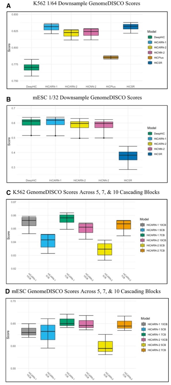
(A) GenomeDISCO scores for 1/64 downsampled K562 Hi-C data for chromosomes 3, 11, 19 and 21. HiCARN-1 achieves an average score (mean ± SD) of 0.8301 ± 0.0070 and HiCARN-2 achieves 0.8210 ± 0.0072. (B) GenomeDISCO scores for 1/32 downsampled mESC Hi-C data for chromosomes 4, 9, 15 and 18. HiCARN-1 achieves an average score (mean ± SD) of 0.5971 ± 0.0569 and HiCARN-2 achieves 0.5802 ± 0.0582. HiCPlus scores are not included for the 1/32 mESC results as they converge to −1, and thus interfere with the scaling of the graph. (C) GenomeDISCO scores from 1/64 downsampled chromosomes 3, 11, 19 and 21 from the K562 cell line across 5, 7 and 10 cascading blocks. (D) GenomeDISCO scores from 1/32 downsampled chromosomes 4, 9, 15 and 18 from the mESC cell line across 5, 7 and 10 cascading blocks
3.3 Differences among varied cascading blocks quantities
We also trained HiCARN with varying numbers of cascading blocks. Using five cascading blocks proved sufficient for outperforming state-of-the-art models, however when more blocks are added, almost all evaluation metric scores slightly increase, especially when predicting across unseen cell lines and species (Fig. 5C and D). We tested the performance of 5, 7 and 10 cascading block networks. HiCARN with 10 cascading blocks outperformed all other architectures at the cost of training and predicting speed. Results for the GM12878 cell line are presented in Supplementary Figure S5. A network of five cascading blocks was chosen to balance the added accuracy of higher block counts and reduced computational cost of lower block counts.
3.4 TAD predictions
TADs are regions on a chromosome generated by chromatin loop extrusions and are contained by boundaries formed from architectural proteins (Beagan and Phillips-Cremins, 2020; Dixon et al., 2016). These structures are helpful for identifying biologically significant regions such as subTADs, microTADs and enhancer–promoter interactions. HiCARN's TAD reconstructions were analyzed using the TopDom TAD detection method (Shin et al., 2016).
HiCARN is also able to closely retain the number (Fig. 6A) and size (Fig. 6B) of HR TADs. Average concordance scores for this region are reported in Table 2. Visualization of the real and predicted TADs within the 40–42.5 Mb region of chromosome 4 displays high overlap between the two (Fig. 7).
Fig. 6.

Comparisons of the number (A) and size (B) of predicted chromosomes compared to the real HR data
Table 2.
Average TAD concordance score for chromosome 4 (40–42.5 Mb) of the GM12878 cell line
| Model | Average concordance score |
|---|---|
| HiCSR | 0.7761 |
| DeepHiC | 0.7834 |
| HiCNN-2 | 0.7322 |
| HiCPlus | 0.7112 |
| HiCARN-1 | 0.8697* |
| HiCARN-2 | 0.84** |
Fig. 8.

3D reconstructions of 1/16 downsampled data, HiCARN-1 and HiCARN-2 contact matrices compared to the 3D reconstruction of real HR contact matrix. The real HR data 3D reconstruction is the centered reconstruction in each image. The region presented is from chromosome 4 (40–45Mb) from the GM12878 cell line
3.5 Chromosome 3D structure reconstruction
We also reconstructed 3D chromatin models using the GenomeFlow structure prediction tool. Models were generated for the 1/16 downsampled matrix, the real HR target, HiCARN-1 and HiCARN-2's predictions for every 5Mb of chromosome 4 (40–190 Mb) from the GM12878 cell line (Fig. 8). PCC and SCC values of HiCARN-1's prediction to the HR target were calculated for each 5-Mb region (Supplementary Fig. S6). HiCARN can produce 3D conformations similar to those of the target contact maps.
Fig. 7.

Overlap comparison of Real HR TAD locations, HiCARN-1 and HiCARN-2's predictions from GM12878 chromosome 4 (40–42.5 Mb). HiCExplorer was used for this visualization
3.6 Chromatin loop detections
Chromatin loops are key regulators in genome transcription (De Laat and Duboule, 2013), thus it is important for enhancement models to accurately detect and predict chromatin loops. At the anchors of these loops are two proteins CTCF and cohesion which have been shown to aid in the formation of loops (Merkenschlager and Nora, 2016).
3.6.1 GM12878 loop detections
Chromatin loops and CTCF anchors were detected for chromosomes 4, 14, 16 and 20 from the GM12878 cell line using the HiCExplorer software (Wolff et al., 2020). We observed that HiCARN models do not overestimate the number of loops detected, thus, maintaining consistency with the number of detected loops in the HR dataset. Supplementary Tables S5–S8 show that HiCARN achieved top performance across three of the four chromosomes tested and second-best performance in the fourth chromosome. Specifically, HiCARN detects >2% of CTCF anchor matches compared to the next performing model on chromosomes 14 and 16, and >1% for chromosome 20. For chromosome 4, HiCARN found 40% CTCF peaks for detected loops, second to HiCSR which found 43% CTCF anchor match. Overall, it was found that HiCARN maintained consistency with the high-resolution data for the number of loops and the percent CTCF matches compared to all other models.
3.6.2 HCT-116 loop detections
To see if our models were able to capture structural genomic differences, HICARN was also trained and tested on cohesion-depleted and untreated HCT-116 cells where cohesion-depleted cells were shown to eliminate loop domains (Rao et al., 2017). After detecting chromatin loops and CTCF anchor matches, we found that HiCARN maintained consistency in the number of loops predicted with CTCF anchors for both cell groups compared to the HR data (Supplementary Tables S9–S12).
4 Conclusion
In this work, we present a novel framework for HR Hi-C contact map predictions. Variations in the number of cascading blocks and the overall framework (CNN versus GAN) do not significantly hinder or improve the performance of HiCARN. However, if the user requires a quick training process, HiCARN-1 with five cascading blocks should be used to reduce computational load during training and predicting.
We also demonstrated HiCARN's superior performance over most existing models in both image and Hi-C evaluation metrics for 1/16, 1/32, 1/64, 1/100 downsampled HR contact maps. The 1/100 downsample results particularly displayed the robustnesses of HiCARN-1, HiCARN-2 and HiCSR for predicting high fidelity images from very low-resolution data. The existing models performed well throughout; however, our network outperformed these models across all tested cell lines. To further confirm the performance consistency of our algorithm, we deliberately selected different chromosomes than our original training, validation and test sets—the chromosome selection for this second test are provided in Supplementary Table S2—and retrained all models. Our results show that HiCARN maintained superior performance, thus showing HiCARN’s robustness across datasets (Supplementary Fig. S7).
TAD, 3D genome structure, and chromatin loop predictions also confirm that HiCARN can proficiently reconstruct biologically significant regions. Overall, HiCARN contributes further to the development of high-fidelity predictions of HR Hi-C contact maps from state-of-the-art resolution enhancement models.
Supplementary Material
Acknowledgements
The authors thank the reviewers for their valuable and constructive comments. They also thank Sean Higgins and Dr Andrew Klocko for their assistance during the manuscript revision phase.
Funding
This work was supported by the National Science Foundation [2050919]. The APC was funded by the Committee on Research and Creative Works (CRCW) Seed Grant funding from the University of Colorado, Colorado Springs [to O.O.]. Any opinions, findings and conclusions or recommendations expressed in this work are those of the author(s) and do not necessarily reflect the views of the National Science Foundation.
Conflict of Interest: none declared.
Contributor Information
Parker Hicks, Department of Biology, Concordia University Irvine, Irvine, CA 92612, USA.
Oluwatosin Oluwadare, Department of Computer Science, University of Colorado, Colorado Springs, CO 80918, USA.
References
- Ahn N. et al. (2018) Fast, accurate, and lightweight super-resolution with cascading residual network. In: Proceedings of European Conference on Computer Vision (ECCV). ECCV 2018: Lecture Notes in Computer Science, Munich, Germany.
- Beagan J.A., Phillips-Cremins J.E. (2020) On the existence and functionality of topologically associating domains. Nat. Genet., 52, 8–16. [DOI] [PMC free article] [PubMed] [Google Scholar]
- Carron L. et al. (2019) Boost-HiC: computational enhancement of long-range contacts in chromosomal contact maps. Bioinformatics, 35, 2724–2729. [DOI] [PubMed] [Google Scholar]
- De Laat W., Duboule D. (2013) Topology of mammalian developmental enhancers and their regulatory landscapes. Nature, 502, 499–506. [DOI] [PubMed] [Google Scholar]
- Dimmick M.C. et al. (2020) HiCSR: a Hi-C super-resolution framework for producing highly realistic contact maps. PhD Thesis, University of Toronto, Toronto, ON, Canada.
- Dixon J.R. et al. (2016) Chromatin domains: the unit of chromosome organization. Mol. Cell, 62, 668–680. [DOI] [PMC free article] [PubMed] [Google Scholar]
- Highsmith M., Cheng J. (2021). VEHiCLE: a variationally encoded Hi-C loss enhancement algorithm for improving and generating Hi-C data. Sci. Rep., 11, 1–13. [DOI] [PMC free article] [PubMed] [Google Scholar]
- Hong H. et al. (2020) DeepHiC: a generative adversarial network for enhancing Hi-C data resolution. PLoS Comput. Biol., 16, e1007287. [DOI] [PMC free article] [PubMed] [Google Scholar]
- Li Z., Dai Z. (2020) SRHiC: a deep learning model to enhance the resolution of Hi-C data. Front. Genet., 11, 353. [DOI] [PMC free article] [PubMed] [Google Scholar]
- Lieberman-Aiden E. et al. (2009) Comprehensive mapping of long-range interactions reveals folding principles of the human genome. Science, 326, 289–293. [DOI] [PMC free article] [PubMed] [Google Scholar]
- Liu T., Wang Z. (2019a) HiCNN: a very deep convolutional neural network to better enhance the resolution of Hi-C data. Bioinformatics, 35, 4222–4228. [DOI] [PMC free article] [PubMed] [Google Scholar]
- Liu T., Wang Z. (2019b) HiCNN2: enhancing the resolution of Hi-C data using an ensemble of convolutional neural networks. Genes, 10, 862. [DOI] [PMC free article] [PubMed] [Google Scholar]
- Liu Q. et al. (2019) hicGAN infers super resolution Hi-C data with generative adversarial networks. Bioinformatics, 35, i99–i107. [DOI] [PMC free article] [PubMed] [Google Scholar]
- Liu B. et al. (2021) Towards faster and stabilized GAN training for high-fidelity few-shot image synthesis. In: International Conference on Learning Representations (ICLR), Vienna, Austria.
- Merkenschlager M., Nora E.P. (2016) CTCF and cohesin in genome folding and transcriptional gene regulation. Annu. Rev. Genomics Hum. Genet., 17, 17–43. [DOI] [PubMed] [Google Scholar]
- Trieu,T. et al. (2019) GenomeFlow: a comprehensive graphical tool for modeling and analyzing 3D genome structure. Bioinformatics, 35(8), 1416–1418. [DOI] [PMC free article] [PubMed] [Google Scholar]
- Oluwadare O. et al. (2019) An overview of methods for reconstructing 3-D chromosome and genome structures from Hi-C data. Biol. Procedures Online, 21, 1–20. [DOI] [PMC free article] [PubMed] [Google Scholar]
- Rao S.S.P. et al. (2014) A 3D map of the human genome at kilobase resolution reveals principles of chromatin looping. Cell, 159, 1665–1680. [DOI] [PMC free article] [PubMed] [Google Scholar]
- Rao S.S. et al. (2017) Cohesin loss eliminates all loop domains. Cell 171, 305–320. [DOI] [PMC free article] [PubMed] [Google Scholar]
- Shin H. et al. (2016) TopDom: an efficient and deterministic method for identifying topological domains in genomes. Nucleic Acids Res., 44, e70. [DOI] [PMC free article] [PubMed] [Google Scholar]
- Ursu O. et al. (2018) GenomeDISCO: a concordance score for chromosome conformation capture experiments using random walks on contact map graphs. Bioinformatics, 34, 2701–2707. [DOI] [PMC free article] [PubMed] [Google Scholar]
- Wolff,J. et al. (2020) Galaxy HiCExplorer 3: a web server for reproducible Hi-C, capture Hi-C and single-cell Hi-C data analysis, quality control and visualization. Nucleic Acids Research, 48(W1), W177–W184. [DOI] [PMC free article] [PubMed]
- Yang T. et al. (2017) HiCRep: assessing the reproducibility of Hi-C data using a stratum-adjusted correlation coefficient. Genome Res., 27, 1939–1949. [DOI] [PMC free article] [PubMed] [Google Scholar]
- Zhang Y. et al. (2018) Enhancing Hi-C data resolution with deep convolutional neural network HiCPlus. Nat. Commun., 9, 1–9. [DOI] [PMC free article] [PubMed] [Google Scholar]
Associated Data
This section collects any data citations, data availability statements, or supplementary materials included in this article.