Abstract
LncRNA and miRNA are two non-coding RNA types that are popular in current research. LncRNA interacts with miRNA to regulate gene transcription, further affecting human health and disease. Accurate identification of lncRNA–miRNA interactions contributes to the in-depth study of the biological functions and mechanisms of non-coding RNA. However, relying on biological experiments to obtain interaction information is time-consuming and expensive. Considering the rapid accumulation of gene information and the few computational methods, it is urgent to supplement the effective computational models to predict lncRNA–miRNA interactions. In this work, we propose a heterogeneous graph inference method based on similarity network fusion (SNFHGILMI) to predict potential lncRNA–miRNA interactions. First, we calculated multiple similarity data, including lncRNA sequence similarity, miRNA sequence similarity, lncRNA Gaussian nuclear similarity, and miRNA Gaussian nuclear similarity. Second, the similarity network fusion method was employed to integrate the data and get the similarity network of lncRNA and miRNA. Then, we constructed a bipartite network by combining the known interaction network and similarity network of lncRNA and miRNA. Finally, the heterogeneous graph inference method was introduced to construct a prediction model. On the real dataset, the model SNFHGILMI achieved AUC of 0.9501 and 0.9426 ± 0.0035 based on LOOCV and 5-fold cross validation, respectively. Furthermore, case studies also demonstrate that SNFHGILMI is a high-performance prediction method that can accurately predict new lncRNA–miRNA interactions. The Matlab code and readme file of SNFHGILMI can be downloaded from https://github.com/cj-DaSE/SNFHGILMI.
LncRNA and miRNA are two non-coding RNA types that are popular in current research.
Introduction
Non-coding RNAs are a class of RNA that does not encode proteins, so for a long time, it was considered a “dark matter” on the genome.1 However, with the accumulation of research, scientists found that only about 2% of the RNA encoded proteins in the human genome and the remaining 98% of the RNA no longer continues to be translated into proteins, but functions in various biological processes as non-coding RNA.2 In the vast majority of human transcript expression, the length of non-coding RNA ranges from 22 nucleotides to hundreds of kb. According to the length of non-coding RNA, the length of more than 200 nucleotides is defined as long non-coding RNA (lncRNA),3 which are involved in various cellular processes such as cell differentiation, growth, death, etc.4 It is also involved in chromatin modification, transcription complex targeting, mRNA splicing and protein translation.5,6 And more and more studies have shown that it is associated with diseases such as gastric cancer, lung cancer, prostate cancer and so on.7,8 MicroRNA (miRNA) is a short non-coding RNA with a length of approximately 22 nucleotides,9 which usually binds to target mRNA or proteins and acts as a negative regulator at the post-transcriptional level. Studies have shown that miRNAs play important roles in biological life processes such as cell growth, tissue differentiation, embryo development and apoptosis, cross-species gene expression variation, and coordinated regulation with transcription factors.10 Both lncRNA and miRNA are closely related to human health and disease.11–15 However, only a few lncRNA/miRNA annotations have experimental information, and there is still a lot of improvement for their research.
LncRNAs have been found can exert biological functions by interacting with DNA, RNA, and proteins.16 Such interactions between lncRNA and biomolecule are very important for the regulation of life activities. Recently, it has been found that lncRNA can act as a sponge of miRNA and reduce the regulation effect of miRNA on mRNA by playing the function of competitive endogenous RNA, thus acting as a decoy to regulate the behavior of miRNA.17,18 Similarly, miRNAs also play an important role in the molecular mechanism of lncRNA.19 Mutual regulation of miRNA and lncRNA has a great influence on the pathological process of human diseases.20 For example, the regulatory network of lncRNA–miRNA in prostate cancer,21 gastric cancer,22 and vascular disease23 has been constructed. However, it is very limited to identify lncRNA–miRNA interaction through biological experiments. To understand the role of lncRNA–miRNA interactions in pathophysiology in more detail and to discover new biomarkers and therapeutic. A reasonable and efficient method for predicting lncRNA–miRNA interaction is necessary.
Recently, there are various computational methods have been developed to predict lncRNA–miRNA interactions. These prediction methods were developed based on the known lncRNA–miRNA heterogeneous network, the similarity network between lncRNAs, and the similarity network between miRNAs. Huang et al. proposed a two-way diffusion model called EPLMI,24 which predicts potential lncRNA–miRNA interactions based on known lncRNA–miRNA interactions and lncRNA/miRNA expression profile information. This is also the first model dedicated to the prediction of lncRNA–miRNA interactions and has made a significant contribution to future research. INLMI is a new model proposed by Huang and Hu based on previous research.25 This model uses network integration on two similarity networks of lncRNA/miRNA, and they predict new lncRNA–miRNA interactions by a non-negative matrix factorization method with integrated network and known lncRNA–miRNA interactions. Zhang et al. proposed a sequence-derived linear neighborhood propagation model (SLNPM).26 This model proposed a novel similarity measure named fast linear neighborhood similarity approach (FLNS) and used the FLNS to calculate the lncRNA–lncRNA similarity and miRNA–miRNA similarity. And then, the label propagation algorithm is introduced to predict the potential lncRNA–miRNA interactions based on the known lncRNA–miRNA interaction, integrated lncRNA similarity, and integrated miRNA similarity. Subsequently, based on previous study, Zhang et al. proposed a sequence-derived linear neighborhood propagation method with information combination for lncRNA–miRNA interaction prediction.27 Compared with SLNPM, this model proposed two strategies of similarity-based information combination and interaction profile-based information combination. Construct two editions of SLNPM based two strategies, and the weighted averages of their results are adopted as final scores. Wong et al. proposed LNRLMI model,28 which constructed a binary network based on known associated lncRNA–miRNA interaction network, lncRNA similarity, and miRNA similarity, and used a semi-supervised learning model called linear neighbor representation method to predict lncRNA–miRNA interaction. Recently, Liu et al. predicted lncRNA–miRNA interactions based on logical matrix factorization with neighborhood regularized.29 Neighborhood regularization takes into account the strong correlation between lncRNA–lncRNA and miRNA–miRNA, and the logical matrix factorization algorithm can use latent vectors to predict potential relationships globally. The combination of the two algorithms further improves the prediction accuracy of the model. In addition, the rich association prediction research in bioinformatics also provide meaningful references for our work (e.g., lncRNA-disease,30–32 miRNA-disease,12,13,33–40 lncRNA–protein,41–43 drug-target,44–47 and drug-disease48–50 interaction prediction). However, although previous work of lncRNA–miRNA interaction prediction has achieved excellent predictions, it is not difficult to find that there are some issues to improve the lncRNA–miRNA interaction prediction. It is noted that the fusion of heterogeneous data is a key factor to improve the accuracy of interaction prediction. Recently, prediction models based on the integration of diverse information and similarity have been proposed and show excellent performance.43,51,52
In this paper, we explored a heterogeneous graph inference method based on similarity network fusion technology, named is SNFHGILMI, to predict lncRNA–miRNA interaction. The similarity network fusion technology was originally proposed by Wang et al.,53 and applied to patient similarity network fusion, which can obtain shared and complementary information from various kernel matrices so that the integrated matrix reveals lncRNA/miRNA information as much as possible. The heterogeneous graph inference algorithm is an iterative process to find the optimal solution based on the similarity information of the global network. All the information about nodes and interactions are expressed on the heterogeneous graph, and only the links of different types of nodes need to be derived to predict lncRNA–miRNA interaction.39,54,55 Based on these two algorithms, the classification model SNFHGILMI was constructed. Specifically, SNFHGILMI firstly integrated the similarity of lncRNA/miRNA based on sequence and interaction profile. Then, based on the integrated lncRNA–lncRNA similarity network, miRNA–miRNA similarity network and known lncRNA–miRNA interaction, a heterogeneous lncRNA–miRNA network was constructed. Finally, a heterogeneous graph inference algorithm was introduced to calculate the lncRNA–miRNA interaction score. The experimental results show that our approach has an excellent performance over other existing methods.
Materials and methods
Datasets
The data used in this work is from the Huang's paper,24 which includes information on known lncRNA–miRNA interactions and the ID of lncRNA/miRNA. The specific information refers to the following three public databases. The database lncRNASNP provides comprehensive information about lncRNA–miRNA interaction, and these known lncRNA–miRNA interactions confirmed by laboratory studies (http://bioinfo.life.hust.edu.cn/lncRNASNP).56 LNCipedia is a comprehensive human lncRNA database (https://lncipedia.org/) containing human lncRNA transcript sequences and annotation information, and lncRNA in this database with a uniform nomenclature system.57 The miRBase is a publicly available database, which provides information of miRNA sequence, annotations and known gene targets (http://www.mirbase.org/index.shtml).58
First, 8091 known lncRNA–miRNA interaction data were collected from the lncRNASNP database. After deleting the duplicate data, and 5118 lncRNA–miRNA entries were obtained. These entries involved 780 lncRNAs and 275 miRNAs. Then, the sequence of each lncRNA was extracted from the LNCipedia database, and only 770 lncRNA sequence information was available. Similarly, the sequence of each miRNA was extracted from the miRBase database. Finally, we removed interaction whose lncRNA sequence is unavailable and 4966 lncRNA–miRNA interactions were obtained as the experimental dataset. Constructing an adjacency matrix A of lncRNA–miRNA interaction. We defined A(i,j) = 1 if lncRNA li interacts with miRNA mj, and A(i,j) = 0 if there is an unknown interaction.
Problem formalization
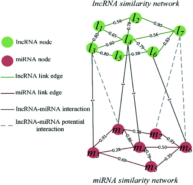
The visualization of the lncRNA–miRNA interaction problem is shown in Fig. 1. Heterogeneous graph consists of nodes and edges. Defined L = {l1, …, li, …, lnl} and M = {m1, …, mj, …, mnm} to represent the nodes of the nl lncRNA and nm miRNA, respectively. Inside the lncRNA (miRNA) network, the weight of the edge is determined by the similarity value of two lncRNA (miRNA) corresponding to two nodes. Between the lncRNA–miRNA networks, if there is an interaction between li and mj, the edge exists and has a weight of 1. Based on the above description, the heterogeneous graph can be represented as G = {{L, M},{Ell, Emm, Elm},{Wll, Wmm, Wlm}}, where Ell, Emm and Elm represent lncRNA–lncRNA, miRNA–miRNA, and lncRNA–miRNA edges, respectively. And Wll, Wmm and Wlm represent the values of the weights on these three kinds of edges. It can be seen that there are missing edges between the lncRNA node and the miRNA node, and these missing edges are unknown lncRNA–miRNA interactions. Our goal is to elucidate new potential lncRNA–miRNA interactions based on lncRNA–lncRNA similarity, miRNA–miRNA similarity and known lncRNA–miRNA interaction.
Fig. 1. Visualization of lncRNA–miRNA interaction heterogeneous network.
Construct lncRNA/miRNA sequence similarity
Similar sequences may have similar structures, and similar structures may have similar functions.59 Based on the hypothesis that functionally similar lncRNA/miRNAs tend to interact with similar miRNA/lncRNA,33 we calculated the lncRNA/miRNA sequence similarity. Here, the sequence global alignment algorithm Needleman–Wunsch is used to calculate and construct the lncRNA/miRNA sequence similarity matrix.60 Referring to previous studies, the parameters are set in the Needleman–Wunsch algorithm as follows, the identification score is 2, the gap-open penalty is −0.5 and the gap-open extending penalty is −0.1. Finally, the sequence similarity matrix of lncRNA is defined as SL, the sequence similarity matrix of miRNA is defined as SM.
Construct lncRNA/miRNA Gaussian interaction profile kernel similarity
Considering that a single similarity network can not provide comprehensive bioinformatics, the Gaussian interaction profile kernel similarity is added here. Given the adjacency matrix Anl×nm of the known lncRNA–miRNA interactions, nl is the number of lncRNA and nm is the number of miRNAs. The interaction profile (IP) of each lncRNA is represented by a row in the adjacency matrix Anl×nm, that is, IP(li) is defined as all elements of the ith row of the adjacency matrix. Similarly, the IP of each miRNA is represented by a column in the adjacency matrix Anl×nm, that is, IP(mj) is defined as all elements of the jth column of the adjacency matrix. Therefore, the Gaussian interaction profile kernel similarity of lncRNA li and lncRNA lj is defined as follows.
| KL(li, lj) = exp(−γl‖IP(li) − IP(lj)‖2) | 1 |
 |
2 |
Here, the parameter γl is used to constrain the bandwidth of the kernel, which is affected by the new bandwidth parameter  The parameter
  is the average number of associations of each lncRNA with the miRNA. Referring to the parameter settings of the previous paper,61 we set
 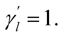 Similarly, the same method is used to construct the Gaussian interaction profile kernel similarity of miRNA.
| KM(mi, mj) = exp(−γm‖IP(mi) − IP(mj)‖2) | 3 |
 |
4 |
Integrate the similarity matrix of lncRNA/miRNA
Using the above similarity calculation method, four similarity matrices are obtained, lncRNA sequence similarity matrix SL, lncRNA Gaussian kernel interaction similarity matrix KL, miRNA sequence similarity matrix SM, miRNA Gaussian kernel interaction similarity matrix KM. It is a key issue that how to use a reasonable and effective method to fuse the two similarity matrices of lncRNA/miRNA so that the information after fusion can better improve the predictive performance of the model. Two matrix fusion methods are given here.
One is a simple linear fusion method called SLF,62 the calculation process is as follows. α is the weight parameter (α is the values between 0 and 1).
| WL(i,j) = α × SL(i,j) + (1 − α) × KL(i,j) | 5 |
| WM(i,j) = α × SM(i,j) + (1 − α) × KM(i,j) | 6 |
The other is a nonlinear combination method called Similarity Network Fusion (SNF), which is used in this paper. This method utilizes the nonlinear iterative method of information to fuse the similarity matrix and achieves good performance.
Considering that the use of discrete data by SNF is not ideal, the lncRNA/miRNA sequence similarity matrix is calculated as follows, so that the values in the matrix are converted to continuous values between 0 and 1.
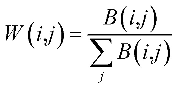 |
7 |
| Wsym = (W + (W)T)/2 | 8 |
Here, B represents the sequence similarity matrix of the lncRNA or miRNA (W)T denotes the transpose of W and making them symmetric using the formula (8). Because of the self-similarity of the diagonal elements of the matrix, the similarity matrix is positively semi-determined by adding a small multiple of identity matrix.45 Finally, the original SL and SM are converted into SLkner and SMkner.
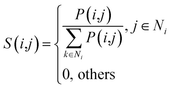
Given four kernel matrices, SLkner, SMkner, KL and KM. Here we take lncRNA as an example to fuse matrix. First, we normalize the kernel matrix by dividing by the sum of the rows, so that the sum of all the elements in each row is 1. Then the normalized matrix is symmetrized by formula (8), and the resulting matrices are defined as P(1) and P(2), corresponding to matrix SLkner and KL, respectively. Next, the K nearest neighbor method is used to calculate the local similarity of the matrix for each P.
 |
9 |
Here, Ni represents the set of neighbors nearest to lncRNA li (including lncRNA li). k is the number of nearest neighbors, and the value of k is set by the user, where k = 3. For neighbors that are not in the nearest neighbor, the value converted to 0. The generated matrices S(1) and S(2) correspond to matrices P(1) and P(2), respectively. This process strengthens the strong links and eliminates weak links in the network, this greatly reduces noise interference.
Finally, after a nonlinear iterative process, the fusion matrices is implemented. The specific process is as follows.
| P(1)t+1 = S(1) × P(2)t × (S(1))T | 10 |
| P(2)t+1 = S(2) × P(1)t × (S(2))T | 11 |
Here, P(1)t+1 is the state matrix transformed by lncRNA sequence kernel matrix after t iteration, and P(2)t+1 is the state matrix transformed by lncRNA Gaussian kernel similarity matrix after t iteration. Each iteration exchanges information of different original networks. After t iterations (in this work t = 20), the final state matrix of lncRNA is calculated as follows.
| WL = (P(1)t + P(2)t)/2 | 12 |
Then, the matrix WL is normalized and further transformed as follows.
| WL = (WL + (WL)T + I)/2 | 13 |
Here, (WL)T denotes the transpose of WL, and I is an identity matrix. Similarly, the fusion of miRNA also uses the above steps. In addition, the fusion method for three or more similarity matrices is not introduced here. For details, please refer to Wang's literature.53
Constructing prediction model
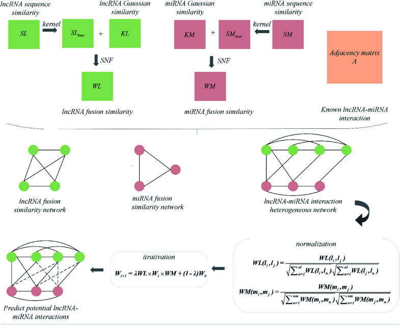
Combining the lncRNA similarity matrix, the miRNA similarity matrix, and the known lncRNA–miRNA interaction matrix, a SNFHGILMI computational model was established to predict potential lncRNA–miRNA interactions. The SNFHGILMI method proposed in this paper combines SNF and heterogeneous graph inference (HGI) algorithms to improve the performance of lncRNA–miRNA interaction prediction. Fig. 2 shows that the lncRNA–miRNA interaction network can combine independent lncRNA and miRNA internal similarities to predict new interactions between lncRNA–miRNAs. That is, if there is no known association between lncRNA li and miRNA mj, then the potential association probability values between them can be solved by the following definition.
 |
14 |
Fig. 2. The flowchart of prediction process of SNFHGILMI.
The above formula indicates that the potential interaction probability between lncRNA li and miRNA mj is calculated by summing all paths of length three (li and ln, mj and mm, ln and mm) in the heterogeneous graph. To obtain the potential interaction probabilities for all unlabeled lncRNA and miRNA pairs in one iteration, we convert the above formula into a multiplication calculation between matrices as follows.
| Wi+1 = λWL × Wi × WM + (1 − λ)W0 | 15 |
Here, λ is a decay factor with a value between 0 and 1. In this work, we set λ = 0.1. W0 is the initial interaction adjacency matrix of lncRNA–miRNA. Each iteration will generate a new interaction matrix. When the matrix difference between Wi+1 and Wi is less than a certain threshold, the matrix converges, which means that the information propagation tends to be stable. According to the previous literature,54 the lncRNA–miRNA correlation probability matrix will converge when the matrices WL and WM are properly normalized using the following formula, respectively.
 |
16 |
 |
17 |
We adopt the threshold as 10−6, which means that when the difference between Wi+1 and Wi measured by the L1 norm is less than 10−6, the iterative process stops and the formula (15) convergence. Moreover, we have given the details of the proof about convergence in the S1 text.†
Results and discussion
Convergence performance
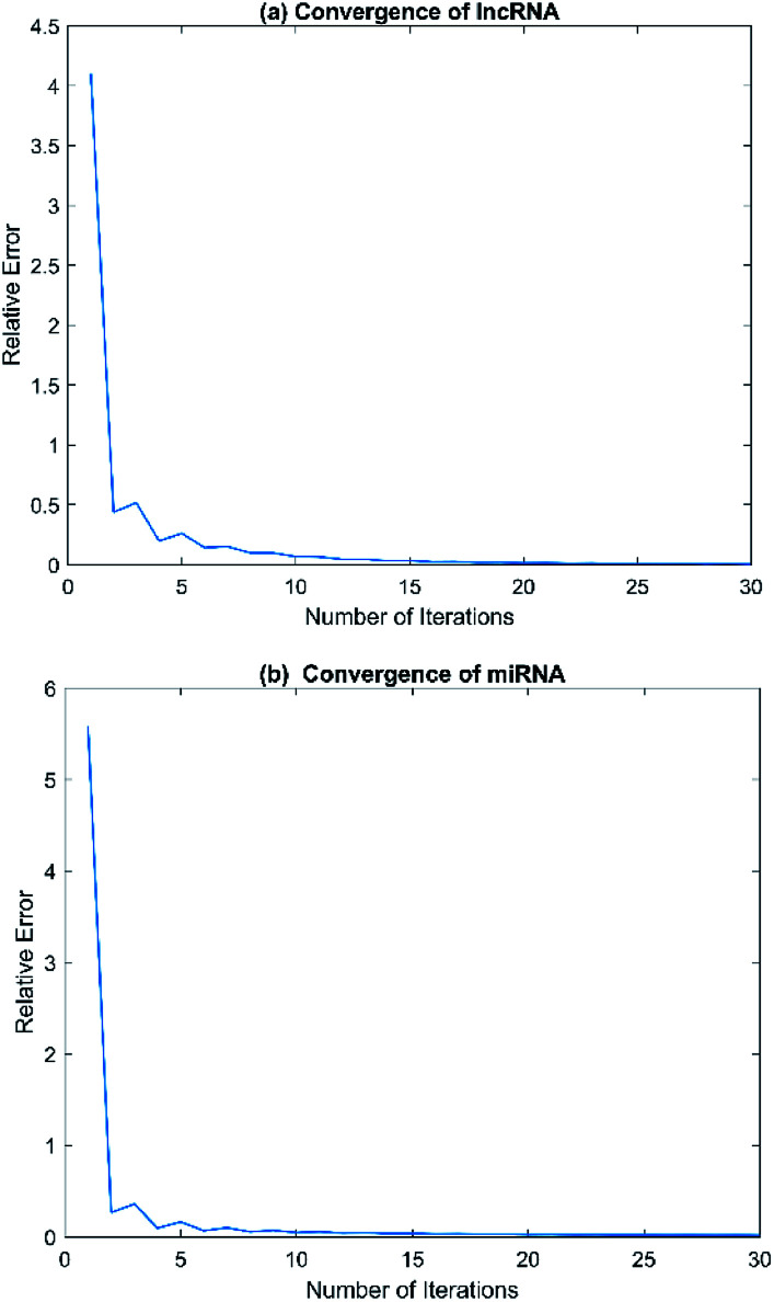
Convergence is a very important problem for iterative algorithms. Therefore, we analyzed the number of iterations of the SNF. Specifically, the experiment defines the relative change index as 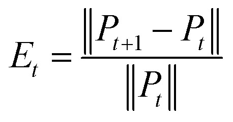 in the iterative process, and the range of t was set to t ∈ {1, 2, 3, …, 28, 29, 30}. The change of relative change index with the number of iterations is shown in Fig. 3. We find that after 15 iterations, the state matrix tends to be stable, which also indicates that the SNF algorithm has good convergence. In this paper, we set the number of iterations t = 20 to ensure sufficient convergence.
Fig. 3. The relative errors of SNF model with different numbers of iteration t. (a) Convergence of lncRNA. (b) Convergence of miRNA.
Parameter settings
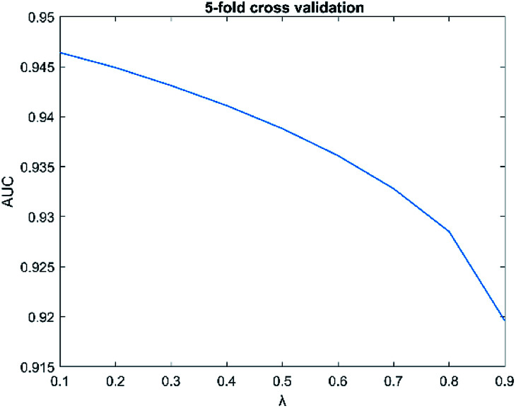
The parameters have a great influence on the performance of the algorithm. There are two parameters in SNFHGILMI, i.e. k and λ. In this section, we will discuss the influence of parameters on the performance of the SNFHGILMI model in a 5-fold cross-validation experiment. K is defined as the number of neighbors. For the selection of parameter k, we set the range k ∈ {1, 2, 3, …, 10}. The AUC value of model SNFHGILMI keeps a small fluctuation range from 0.001 to 0.005, we finally choose parameter k = 3. λ is a decay factor, and the range of λ is set to λ ∈ {0.1, 0.2, 0.3, …, 0.9}. The change of the AUC value of the model SNFHGILMI with the parameter λ is shown in Fig. 4. When λ = 0.1, the model has high prediction performance.
Fig. 4. The influence of parameters λ on model performance.
Performance evaluation for SNFHGILMI
5-foldCV (5-fold cross validation) and LOOCV (Leave One Out cross validation) are two popular methods to evaluate the performance of the model. In this paper, these two methods are also used to evaluate the performance of our proposed computational model SNFHGILMI. Area under the Receiver Operator Characteristics curve (AUC) is an important metrics to evaluate classification models. In addition, there are several popular metrics, i.e. sen, acc, F 1-score.
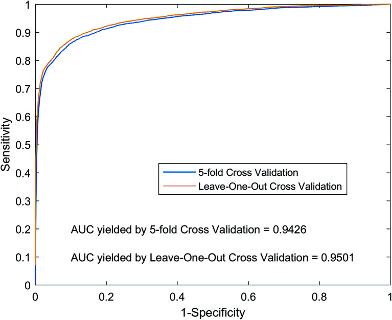
For LOOCV, each known lncRNA–miRNA interaction is taken as a test sample, and all remaining known interactions are used as training samples to construct a prediction model. We compare and rank the test sample prediction scores with the all unknown interaction lncRNA–miRNA in the dataset. If the score is higher than the given threshold, we will consider the test sample to be a positive sample. For each of the different thresholds set in the experiment, we obtained the corresponding true positive rate (TPR, sensitivity) and false positive rate (FPR, specificity). As shown in Fig. 5, we plot the TPR and FPR values under different thresholds to obtain the ROC curve (Receiver Operating Curves), and we calculate the value of AUC. Implementing LOOCV on the SNFHGILMI, we have an AUC value of 0.9501. For 5-foldCV, the lncRNA–miRNA interaction was randomly divided into equal 5 subsets. Then, one subset was selected as the test sample in turn, and the remaining four subsets were used as the training samples to construct the prediction model. In order to avoid the error caused by randomly dividing data, the calculation model SNFHGILMI was verified by 5-foldCV for 100 times, and the average of AUC was used as the final prediction performance. As shown in Fig. 5, SNFHGILMI's average AUC values are 0.9426 ± 0.0015.
Fig. 5. Performance comparison by using SNFHGILMI in the framework of 5-foldCV and LOOCV.
Comparison among different similarity network integrate methods
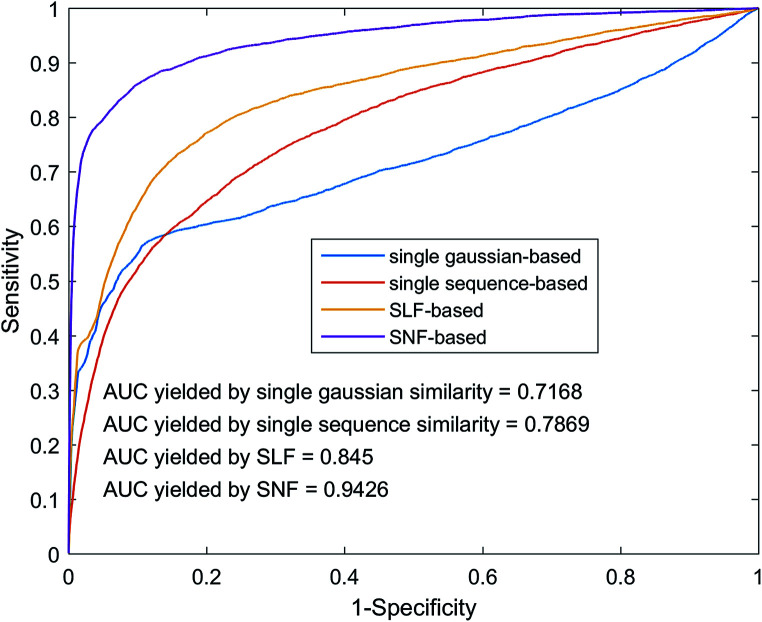
The fusion of similarity networks is a very important part of the model construction process. In order to prove the superiority of the SNF method, the model was constructed using SLF and SNF, respectively. The performance of the above two models on the benchmark dataset was evaluated using 5-foldCV. As shown in Fig. 6, the model based on the SNF is significantly better than the model based on the SLF, which shows that SNF can share and complement the kernel matrix information more effectively and improve the prediction performance of the model. In addition, model performance based on SNF and SLF methods is superior to model performance based on single sequence information or single Gaussian interaction profile kernel information, which also illustrates the importance of similarity network fusion from another aspect.
Fig. 6. Performance comparison among different similarity network integrates methods by using heterogeneous graph.
Compared with other methods
To further demonstrate the good performance of the model SNFHGILMI. We compared SNFHGILMI method with other state-of-the-art methods and some network-based methods. Among them, EPLMI calculated the expression profiles similarity of lncRNA and miRNA, and constructs a model based on the network two-way diffusion algorithm. INLMI integrates sequence similarity and expression profile similarity of lncRNA and miRNA, and constructs a model using non-negative matrix factorization. In addition, we also compared SNFHGILMI method with some classical network propagation algorithms such as RWR (Random Walk with Restart),63 LncCF (LncRNA-based collaborative filtering) and MiCF (MiRNA-based collaborative filtering) that were widely used in bioinformatics.64 RWR simulates a random walker that randomly transitions from the current seed node to the neighbor nodes, and can return to the start node with a given restart probability. LncCF and MiCF are based on the same assumption that if a lncRNA (miRNA) interacts with a miRNA (lncRNA), similar lncRNAs (miRNAs) tend to interact with this miRNA (lncRNA). On the benchmark dataset, 5foldCV was used for evaluation of all model's performance, and the results are shown in Table 1. Our method achieved an AUC value of 0.9457, which was significantly higher than EPLMI, INLMI, RWR, LncCF, and MiCF. The results show that SNFHGILMI has reliable and effective prediction performance.
Performance comparison among different methods by using SNFHGILMI in the framework of 5-foldCV.
| Method | AUC | SEN | ACC | F1 |
|---|---|---|---|---|
| EPLMI | 0.8451 | 0.1343 | 0.9940 | 0.1078 |
| INLMI | 0.8523 | 0.1541 | 0.9938 | 0.1085 |
| RWR | 0.9231 | 0.3841 | 0.9951 | 0.4283 |
| LncCF | 0.7847 | 0.3051 | 0.9963 | 0.4403 |
| MiCF | 0.8727 | 0.2823 | 0.9932 | 0.2824 |
| SNFHGILMI | 0.9457 | 0.4882 | 0.9959 | 0.5318 |
Case studies
We conducted case studies in known lncRNA–miRNA interaction to further validate the predictive capability of the model. Here, lnc-CHSY1-5:1 and hsa-miR-17-5p were selected as candidate prediction objects, respectively. The lncRNA lnc-CHSY1-5:1 is associated with breast cancer, which is the leading cause of cancer death in women worldwide.65 The miRNA hsa-miR-17-5p is associated with a variety of cancers and can act as both oncogene and suppressor genes in different cellular environments.66 As shown in Table 2, for lncRNA lnc-CHSY1-5:1, all miRNAs are sorted according to the interaction score predicted by the model, and the top miRNAs will have a greater probability of interacting with lnc-CHSY1-5:1. We selected the top 10 potential miRNAs, and six of them have been confirmed by biochemical experiments to be searched in starBasev2.0 and lncRNASNP2. Similarly, as shown in Table 3, for miRNA hsa-mir-17-5p, seven of the top 10 potential lncRNAs have been confirmed by biochemical experiments. This shows that our model can effectively predict new potential interactions.
Top 10 predictions for lnc-CHSY1-5:1 by SNFHGILMI.
| No. | LncRNA | Confirmed? |
|---|---|---|
| 1 | lnc-SLTM-3:1 | YES |
| 2 | lnc-CPT2-3:1 | |
| 3 | lnc-LRIG1-2:1 | |
| 4 | lnc-FAS-1:1 | YES |
| 5 | lnc-CALCOCO2-3:1 | YES |
| 6 | lnc-MYC-2:16 | |
| 7 | lnc-KB-1507C5.2.1-3:3 | YES |
| 8 | lnc-ACER2-1:1 | YES |
| 9 | lnc-RPGRIP1L-1:1 | YES |
| 10 | lnc-PIGM-1:1 | YES |
Top 10 predictions for hsa-miR-17-5p by SNFHGILMI.
| No. | MiRNA | Confirmed? |
|---|---|---|
| 1 | hsa-miR-424-5p | YES |
| 2 | hsa-miR-195-5p | YES |
| 3 | hsa-miR-15a-5p | YES |
| 4 | hsa-miR-15b-5p | YES |
| 5 | hsa-miR-485-5p | |
| 6 | hsa-miR-24-3p | |
| 7 | hsa-miR-421 | |
| 8 | hsa-miR-27a-3p | YES |
| 9 | hsa-miR-155-5p | |
| 10 | hsa-miR-27b-3p | YES |
Conclusions
LncRNA–miRNA interactions can reveal various biological functions and mechanisms. Therefore, the study of lncRNA–miRNA interactions is an important direction. At present, only some experimental data and a few calculation methods still have great limitations on the study of lncRNA–miRNA. It is urgent to propose more computational methods to predict novel lncRNA–miRNA interactions. Compare with other state-of-the-art methods, the SNFHGILMI method proposed in this work has the following advantages: (1) it integrates similarity data using a nonlinear network fusion technology, which not only characterizes the valuable information of each individual network but also shows better performance when combining two or more networks without obvious linear relationship; (2) all the information about lncRNA, miRNA and lncRNA–miRNA interactions are expressed on the heterogeneous graph, and only the links of different types of nodes need to be derived; (3) the heterogeneous graph inference algorithm can be used to predictions for new lncRNAs which have no known related miRNAs and miRNAs without any known associated lncRANs; (4) it converted iterative process into matrix multiplications, which can predict potential interactions score for all lncRNA–miRNA pairs simultaneously. The performance of the model was evaluated by LOOCV and 5-foldCV on the benchmark dataset. The experimental results show that our method has excellent performance in predicting lncRNA–miRNA interactions.
Although SNFHGILMI showed good performance in lncRNA–miRNA prediction as described above, it still has some limitations. SNFHGILMI used two lncRNA-related and two miRNA-related information to integrate the lncRNA/miRNA similarity matrices, we hope that more information (e.g., lncRNA/miRNA functional annotations, lncRNA/miRNA expression profile) will be used to integrate similarity matrices. In addition, the SNFHGILMI relies on known interactions, we expect lncRNA and miRNA are well studied further to better predict lncRNA–miRNA interactions.
Conflicts of interest
There are no conflicts to declare.
Supplementary Material
Acknowledgments
This work was supported by the National Natural Science Foundation of China (Grant No. 61762026, 61462018), the Guangxi Provincial Natural Science Foundation (Grant No. 2017GXNSFAA198278), the Innovation Project of GUET Graduate Education (Grant No. 2018YJCX47 and 2019YCXS056), the Guangxi Key Laboratory of Trusted Software (Grant No. kx201403), the Guangxi Colleges and Universities Key Laboratory of Intelligent Processing of Computer Images and Graphics (Grant No. GIIP201502).
Electronic supplementary information (ESI) available. See DOI: 10.1039/c9ra11043g
References
- Adelman K. Egan E. Nature. 2017;543:183. doi: 10.1038/543183a. [DOI] [PubMed] [Google Scholar]
- Yamamura S. Imai-Sumida M. Tanaka Y. Dahiya R. Cell. Mol. Life Sci. 2018;75:467–484. doi: 10.1007/s00018-017-2626-6. [DOI] [PMC free article] [PubMed] [Google Scholar]
- Liao Q., Bu D., Sun L., Luo H. and Zhao Y., in Health Informatics Data Analysis, Springer, 2017, pp. 51–60 [Google Scholar]
- Li J. Tian H. Yang J. Gong Z. DNA Cell Biol. 2016;35:459–470. doi: 10.1089/dna.2015.3187. [DOI] [PubMed] [Google Scholar]
- Engreitz J. M. Haines J. E. Perez E. M. Munson G. Chen J. Kane M. McDonel P. E. Guttman M. Lander E. S. Nature. 2016;539:452. doi: 10.1038/nature20149. [DOI] [PMC free article] [PubMed] [Google Scholar]
- Chen L. Zhang Y.-H. Pan X. Liu M. Wang S. Huang T. Cai Y.-D. Int. J. Mol. Sci. 2018;19:3416. doi: 10.3390/ijms19113416. [DOI] [PMC free article] [PubMed] [Google Scholar]
- Huang Y.-A. Chen X. You Z.-H. Huang D.-S. Chan K. C. Oncotarget. 2016;7:25902–25914. doi: 10.18632/oncotarget.8296. [DOI] [PMC free article] [PubMed] [Google Scholar]
- Pan X. Jensen L. J. Gorodkin J. Bioinformatics. 2018;35:1494–1502. doi: 10.1093/bioinformatics/bty859. [DOI] [PubMed] [Google Scholar]
- Panwar B. Omenn G. S. Guan Y. Bioinformatics. 2017;33:1554–1560. doi: 10.1093/bioinformatics/btx019. [DOI] [PMC free article] [PubMed] [Google Scholar]
- Gebert L. F. MacRae I. J. Nat. Rev. Mol. Cell Biol. 2019;20:21–37. doi: 10.1038/s41580-018-0045-7. [DOI] [PMC free article] [PubMed] [Google Scholar]
- Pan X. Shen H.-B. bioRxiv. 2019:666719. [Google Scholar]
- Chen X. Xie D. Wang L. Zhao Q. You Z.-H. Liu H. Bioinformatics. 2018;34:3178–3186. doi: 10.1093/bioinformatics/bty333. [DOI] [PubMed] [Google Scholar]
- Chen X. Xie D. Zhao Q. You Z.-H. Briefings Bioinf. 2019;20:515–539. doi: 10.1093/bib/bbx130. [DOI] [PubMed] [Google Scholar]
- Chen X. Yan C. C. Zhang X. You Z.-H. Briefings Bioinf. 2017;18:558–576. doi: 10.1093/bib/bbw060. [DOI] [PMC free article] [PubMed] [Google Scholar]
- Chen X. Sun Y.-Z. Guan N.-N. Qu J. Huang Z.-A. Zhu Z.-X. Li J.-Q. Briefings Funct. Genomics. 2019;18:58–82. doi: 10.1093/bfgp/ely031. [DOI] [PubMed] [Google Scholar]
- Atianand M. K. Fitzgerald K. A. Trends Mol. Med. 2014;20:623–631. doi: 10.1016/j.molmed.2014.09.002. [DOI] [PMC free article] [PubMed] [Google Scholar]
- Militello G. Weirick T. John D. Döring C. Dimmeler S. Uchida S. Briefings Bioinf. 2016;18:780–788. doi: 10.1093/bib/bbw053. [DOI] [PubMed] [Google Scholar]
- Li D. Ainiwaer J. Sheyhiding I. Zhang Z. Zhang L. Eur. Rev. Med. Pharmacol. Sci. 2016;20:2285–2295. [PubMed] [Google Scholar]
- Paraskevopoulou M. D. and Hatzigeorgiou A. G., in Long Non-Coding RNAs, Springer, 2016, pp. 271–286 [Google Scholar]
- Liz J. Esteller M. Biochim. Biophys. Acta, Gene Regul. Mech. 2016;1859:169–176. doi: 10.1016/j.bbagrm.2015.06.015. [DOI] [PubMed] [Google Scholar]
- Ma G. Tang M. Wu Y. Xu X. Pan F. Xu R. Am. J. Transl. Res. 2016;8:5141. [PMC free article] [PubMed] [Google Scholar]
- Mao Y. Liu R. Zhou H. Yin S. Zhao Q. Ding X. Wang H. Cancer Gene Ther. 2017;24:267. doi: 10.1038/cgt.2017.14. [DOI] [PubMed] [Google Scholar]
- Li M. Duan L. Li Y. Liu B. Life Sci. 2019;233:116440. doi: 10.1016/j.lfs.2019.04.066. [DOI] [PubMed] [Google Scholar]
- Huang Y.-A. Chan K. C. You Z.-H. Bioinformatics. 2017;34:812–819. doi: 10.1093/bioinformatics/btx672. [DOI] [PMC free article] [PubMed] [Google Scholar]
- Hu P., Huang Y.-A., Chan K. C. and You Z.-H., International Conference on Intelligent Computing. Springer, Cham, 2018 [Google Scholar]
- Zhang W., Tang G., Wang S., Chen Y., Zhou S. and Li X., 2018 IEEE International Conference on Bioinformatics and Biomedicine (BIBM). IEEE, 2018 [Google Scholar]
- Zhang W. Tang G. Zhou S. Niu Y. BMC Genomics. 2019;20:1–12. doi: 10.1186/s12864-018-5379-1. [DOI] [PMC free article] [PubMed] [Google Scholar]
- Wong L. Huang Y. A. You Z. H. Chen Z. H. Cao M. Y. J. Cell. Mol. Med. 2020;24:79–87. doi: 10.1111/jcmm.14583. [DOI] [PMC free article] [PubMed] [Google Scholar]
- Liu H. Ren G. Chen H. Liu Q. Yang Y. Zhao Q. Knowl. Base Syst. 2020;191:105261. doi: 10.1016/j.knosys.2019.105261. [DOI] [Google Scholar]
- Yu J. Xuan Z. Feng X. Zou Q. Wang L. BMC Bioinf. 2019;20(1):396. doi: 10.1186/s12859-019-2985-0. [DOI] [PMC free article] [PubMed] [Google Scholar]
- Fu G. Wang J. Domeniconi C. Yu G. Bioinformatics. 2018;34:1529–1537. doi: 10.1093/bioinformatics/btx794. [DOI] [PubMed] [Google Scholar]
- Lu C. Yang M. Luo F. Wu F.-X. Li M. Pan Y. Li Y. Wang J. Bioinformatics. 2018;34:3357–3364. doi: 10.1093/bioinformatics/bty327. [DOI] [PubMed] [Google Scholar]
- Chen X. Wang L. Y. Huang L. J. Cell. Mol. Med. 2018;22:2884–2895. doi: 10.1111/jcmm.13583. [DOI] [PMC free article] [PubMed] [Google Scholar]
- Chen X. Gong Y. Zhang D. You Z. Li Z. e. J. Cell. Mol. Med. 2018:472–485. doi: 10.1111/jcmm.13336. [DOI] [PMC free article] [PubMed] [Google Scholar]
- Chen X. Wu Q.-F. Yan G.-Y. RNA Biol. 2017;14:952–962. doi: 10.1080/15476286.2017.1312226. [DOI] [PMC free article] [PubMed] [Google Scholar]
- Liang C. Yu S. Luo J. PLoS Comput. Biol. 2019;15:e1006931. doi: 10.1371/journal.pcbi.1006931. [DOI] [PMC free article] [PubMed] [Google Scholar]
- Chen X. Huang L. Xie D. Zhao Q. Cell Death Dis. 2018;9:1–16. doi: 10.1038/s41419-017-0012-9. [DOI] [PMC free article] [PubMed] [Google Scholar]
- Chen X. Huang L. PLoS Comput. Biol. 2017;13:e1005912. doi: 10.1371/journal.pcbi.1005912. [DOI] [PMC free article] [PubMed] [Google Scholar]
- Chen X. Yin J. Qu J. Huang L. PLoS Comput. Biol. 2018;14:e1006418. doi: 10.1371/journal.pcbi.1006418. [DOI] [PMC free article] [PubMed] [Google Scholar]
- Chen X. Wang L. Qu J. Guan N.-N. Li J.-Q. Bioinformatics. 2018;34:4256–4265. doi: 10.1093/bioinformatics/bty503. [DOI] [PubMed] [Google Scholar]
- Zhao Q. Zhang Y. Hu H. Ren G. Zhang W. Liu H. Front. Genet. 2018;9:239. doi: 10.3389/fgene.2018.00239. [DOI] [PMC free article] [PubMed] [Google Scholar]
- Zhang W. Qu Q. Zhang Y. Wang W. Neurocomputing. 2018;273:526–534. doi: 10.1016/j.neucom.2017.07.065. [DOI] [Google Scholar]
- Zhang W. Yue X. Tang G. Wu W. Huang F. Zhang X. PLoS Comput. Biol. 2018;14:e1006616. doi: 10.1371/journal.pcbi.1006616. [DOI] [PMC free article] [PubMed] [Google Scholar]
- Zong N. Kim H. Ngo V. Harismendy O. Bioinformatics. 2017;33:2337–2344. doi: 10.1093/bioinformatics/btx160. [DOI] [PMC free article] [PubMed] [Google Scholar]
- Chen X. Yan C. C. Zhang X. Zhang X. Dai F. Yin J. Zhang Y. Briefings Bioinf. 2016;17:696–712. doi: 10.1093/bib/bbv066. [DOI] [PubMed] [Google Scholar]
- Ezzat A. Wu M. Li X.-L. Kwoh C.-K. Briefings Bioinf. 2019;20:1337–1357. doi: 10.1093/bib/bby002. [DOI] [PubMed] [Google Scholar]
- Olayan R. S. Ashoor H. Bajic V. B. Bioinformatics. 2018;34:1164–1173. doi: 10.1093/bioinformatics/btx731. [DOI] [PMC free article] [PubMed] [Google Scholar]
- Zhang W. Yue X. Lin W. Wu W. Liu R. Huang F. Liu F. BMC Bioinf. 2018;19:233. doi: 10.1186/s12859-018-2220-4. [DOI] [PMC free article] [PubMed] [Google Scholar]
- Zhang W. Yue X. Huang F. Liu R. Chen Y. Ruan C. Methods. 2018;145:51–59. doi: 10.1016/j.ymeth.2018.06.001. [DOI] [PubMed] [Google Scholar]
- Zhang W. Yue X. Lin W. Wu W. Liu R. Huang F. Liu F. BMC Bioinf. 2018;19:1–12. doi: 10.1186/s12859-017-2006-0. [DOI] [PMC free article] [PubMed] [Google Scholar]
- Zhang W. Jing K. Huang F. Chen Y. Li B. Li J. Gong J. Inf. Sci. 2019;497:189–201. doi: 10.1016/j.ins.2019.05.017. [DOI] [Google Scholar]
- Zhang W. Li Z. Guo W. Yang W. Huang F. IEEE/ACM Trans. Comput. Biol. Bioinf. 2019 doi: 10.1109/TCBB.2019.2931546. [DOI] [Google Scholar]
- Wang B. Mezlini A. M. Demir F. Fiume M. Tu Z. Brudno M. Haibe-Kains B. Goldenberg A. Nat. Methods. 2014;11:333. doi: 10.1038/nmeth.2810. [DOI] [PubMed] [Google Scholar]
- Chen X. Yan C. C. Zhang X. You Z.-H. Huang Y.-A. Yan G.-Y. Oncotarget. 2016;7:65257–65269. doi: 10.18632/oncotarget.11251. [DOI] [PMC free article] [PubMed] [Google Scholar]
- Yin J. Chen X. Wang C.-C. Zhao Y. Sun Y.-Z. Mol. Pharmaceutics. 2019;16:3157–3166. doi: 10.1021/acs.molpharmaceut.9b00384. [DOI] [PubMed] [Google Scholar]
- Gong J. Liu W. Zhang J. Miao X. Guo A.-Y. Nucleic Acids Res. 2014;43:D181–D186. doi: 10.1093/nar/gku1000. [DOI] [PMC free article] [PubMed] [Google Scholar]
- Volders P.-J. Verheggen K. Menschaert G. Vandepoele K. Martens L. Vandesompele J. Mestdagh P. Nucleic Acids Res. 2014;43:D174–D180. doi: 10.1093/nar/gku1060. [DOI] [PMC free article] [PubMed] [Google Scholar]
- Kozomara A. Griffiths-Jones S. Nucleic Acids Res. 2013;42:D68–D73. doi: 10.1093/nar/gkt1181. [DOI] [PMC free article] [PubMed] [Google Scholar]
- Chen J.-L. Blasco M. A. Greider C. W. Cell. 2000;100:503–514. doi: 10.1016/S0092-8674(00)80687-X. [DOI] [PubMed] [Google Scholar]
- Likic V., Lecture given at the 7th Melbourne Bioinformatics Course, Bi021 Molecular Science and Biotechnology Institute, University of Melbourne, 2008, pp. 1–46 [Google Scholar]
- You Z.-H. Huang Z.-A. Zhu Z. Yan G.-Y. Li Z.-W. Wen Z. Chen X. PLoS Comput. Biol. 2017;13:e1005455. doi: 10.1371/journal.pcbi.1005455. [DOI] [PMC free article] [PubMed] [Google Scholar]
- van Laarhoven T. Nabuurs S. B. Marchiori E. Bioinformatics. 2011;27:3036–3043. doi: 10.1093/bioinformatics/btr500. [DOI] [PubMed] [Google Scholar]
- Lee I. Nam H. BMC Bioinf. 2018;19:208. doi: 10.1186/s12859-018-2199-x. [DOI] [PMC free article] [PubMed] [Google Scholar]
- Zheng X. Wang Y. Tian K. Zhou J. Guan J. Luo L. Zhou S. BMC Bioinf. 2017;18:420. doi: 10.1186/s12859-017-1819-1. [DOI] [PMC free article] [PubMed] [Google Scholar]
- Yao Q. Wu L. Li J. guang Yang L. Sun Y. Li Z. He S. Feng F. Li H. Li Y. Sci. Rep. 2017;7:39516. doi: 10.1038/srep39516. [DOI] [PMC free article] [PubMed] [Google Scholar]
- Cloonan N. Brown M. K. Steptoe A. L. Wani S. Chan W. L. Forrest A. R. Kolle G. Gabrielli B. Grimmond S. M. Genome Biol. 2008;9:R127. doi: 10.1186/gb-2008-9-8-r127. [DOI] [PMC free article] [PubMed] [Google Scholar]
Associated Data
This section collects any data citations, data availability statements, or supplementary materials included in this article.


