Cramér-Rao bound-informed training of neural networks for quantitative MRI

Abstract

Purpose:

To improve the performance of neural networks for parameter estimation in quantitative MRI, in particular when the noise propagation varies throughout the space of biophysical parameters.

Theory and Methods:

A theoretically well-founded loss function is proposed that normalizes the squared error of each estimate with respective CramÃl’r-Rao bound (CRB)—a theoretical lower bound for the variance of an unbiased estimator. This avoids a dominance of hard-to-estimate parameters and areas in parameter space, which are often of little interest. The normalization with corresponding CRB balances the large errors of fundamentally more noisy estimates and the small errors of fundamentally less noisy estimates, allowing the network to better learn to estimate the latter. Further, proposed loss function provides an absolute evaluation metric for performance: A network has an average loss of 1 if it is a maximally-efficient unbiased estimator, which can be considered the ideal performance. The performance gain with proposed loss function is demonstrated at the example of an 8-parameter magnetization transfer model that is fitted to phantom and in vivo data.

Results:

Networks trained with proposed loss function perform close to optimal, i.e. their loss converges to approximately 1, and their performance is superior to networks trained with the standard mean-squared error (MSE). The proposed loss function reduces the bias of the estimates compared to the MSE loss, and improves the match of the noise variance to the CRB. This performance gain translates to in vivo maps that align better with literature.

Conclusion:

Normalizing the squared error with the Cramér-Rao bound during the training of neural networks improves their performance in estimating biophysical parameters.

1 |. INTRODUCTION

Quantitative MRI (qMRI) characterizes the spin physics in biological tissue with the aim to provide quantitative biomarkers for pathological changes^1,2,3. qMRI entails fitting a biophysical model to a signal curve, and this model fitting is usually a non-convex problem, which is traditionally solved via non-linear least squares (NLLS) fitting. It depends on the initialization and requires iterative searches for the best fit, thereby, it can get stuck in a local minimum. Besides this risk, NLLS is often prohibitively slow for clinical routine imaging⁴. Computation speed is particularly problematic for complex transient-state models that have been popularized by Magnetic Resonance Fingerprinting (MRF)⁵.

MRF outsources the slow simulations to the precomputation of a dictionary, which is then matched to the measured signal. This approach equals a brute force grid search, which also overcomes the issue of a non-convex optimization landscape. Although dictionary matching ensures finding the global optimum within the simulated dictionary, it has known practical challenges, such as discretization errors and the so-called curse of dimensionality. The latter describes the exponentially increasing memory and computation time requirements with a growing number of biophysical parameters^6,7.

The computational burden of dictionary matching can be reduced by singular value decomposition (SVD) and compressed sensing techniques^8,9,10,11,12. Nonetheless, these improvements do not overcome the curse of dimensionality and the computational burden is prohibitive for models with many parameters, such as the magnetization transfer (MT) model used here, which has overall 8 parameters. In contrast, the curse of dimensionality can be overcome with dictionary-free regression methods^13,14, as well as deep learning (DL). As a result, these methods are very fast once the network has been trained. As the parameter fitting in both of these methods is feed-forward without initialization dependency. Instead of fitting an estimate using an iterative optimization procedure, neural networks apply a learned function. Yet, the extensive literature on machine learning indicates that lifting the problem to a high-dimensional space usually results in many minima with comparable performance, i.e. each minima represents a different network that produces similar estimates. Therefore, we are less dependant on the convergence to a global minimum¹⁵

Because of those advantages over NLLS fitting and dictionary matching, these methods gained a lot of attention recently, in particular DL^{16,17,18,19,20,21,22,6,23,7,24}: e.g., the DRONE²⁰ method maps the magnitudes of fingerprints to T₁ and T₂ maps with a four-layer fully connected network (FCN). Virtue et al.¹⁹ designed a three-layer FCN, which processes complex-valued data. During training, they augment the data with undersampling artifacts, which are heuristically derived from in vivo data. Additionally, convolutional neural networks^25,21,6 and recurrent neural networks²² have been proposed to exploit the temporally local structure of the fingerprints. Inspired by the work of McGivney et al.²⁶, who showed that MRF dictionaries are often low rank, Golbabaee et al.²³ trained a neural network with a first layer fixed to the singular vectors associated with the highest singular values. In⁷, image reconstruction is performed by solving a regularized version of an optimization problem with a low rank constraint, followed by a deep non-local residual convolutional neural network to restore parameter maps.

Most of the above described methods use the mean squared error (MSE) as the objective function during training, which aims to minimize the sum of the squared differences between each parameter and its estimate^{18,7,20,19,22,25,21,6,23}. However, this loss has natural weaknesses for parameter estimation: different parameters are at different scales and have different dimensions. For example, _T1 values are about 10 times larger than _T2. As a result, _T1 can dominate the MSE loss during the training of a network that jointly estimates both parameters^16,17. When estimating parameters of different physical dimensions, such as the fractional proton density $m_0^s$ (cf. Section 2.3) and the relaxation times, using MSE as loss function becomes even more questionable from a physics perspective. Indeed, the use of MSE in this context violates the well-known homogeneity principle which states that two quantities with different dimensions cannot be added up.

These problems can be overcome with the mean relative absolute error as suggested in Refs.^16,17,27, or by training separate networks to estimate each parameter. Another problem is, however, not addressed by the mean relative absolute error: it is often easier to estimate one biophysical parameter within a specific range of parameters, than it is in other ranges. To give an example, the estimation of _T1 usually becomes increasingly difficult at short _T2-times as this reduces the overall signal to noise ratio. While this example is rather pictorial, the ease of parameter estimation is not always intuitive and gives rise to the same problem described above: the MSE is dominated by areas in parameter space where the estimate has large errors and these areas are usually not the ones of interest, in particular when using a pulse sequence that was optimized for a certain area in parameter space^{28,29,30,31,32}. In such areas of parameter space, the inverse problem is ill-conditioned and the variance of the estimate will be large. As a consequence, the MSE loss in standard deep-learning methods may be dominated by the contribution of those pathological regions of the parameter space. Gradients used in the back-propagation mostly account for those hard-to-estimate samples, which prevents the training for the majority of the parameter space, where the inverse problem is better conditioned. A loss function with CRB normalization mitigates this issue.

In this paper, we introduce a theoretically grounded loss function that ensures close to optimal performance even in heterogeneous and high-dimensional parameter spaces. We will demonstrate that the proposed loss function fulfills these requirements by normalizing the squared error of each estimate with respective Cramér-Rao bound (CRB)^33,34, a theoretical lower bound for the variance of an unbiased estimator.

In Section 2 we introduce the CRB-weighted loss function while connecting neural-network (NN)-based parameter estimation back to signal processing theory. In Section 3, we show that our approach can jointly and efficiently predict multiple parameters in a high-dimensional parameter 3 space, and we compare it to the commonly used MSE loss. We elaborate the advantages and disadvantages of the proposed loss function in Section 4. Code for replicating the proposed work will be available on https://github.com/quentin-duchemin/MRF-CRBLoss. The most updated version of code for fingerprints simulation used in this paper is available on https://github.com/JakobAsslaender/MRIgeneralizedBloch.jl³⁵.

2 |. METHOD

2.1 |. The CramÃl’r-Rao bound (CRB)

First, we recap the definition of the Cramér-Rao Bound and some of its properties that are useful for this paper. We consider a biophysical model with P parameters and we denote the fingerprint corresponding to any set of tissue parameters $\left({\theta }_1,\dots ,{\theta }_P\right)\in {ℝ}^P$ by $\mathbf{x}\left({\theta }_1,\dots ,{\theta }_P\right)\in {ℂ}^d$, where d is the number of data points in the fingerprint. We assume that for some tissue parameters (θ_{1, … ,}θ_P) we observe a normally distributed random vector X with mean x₍θ_{1, … ,}θ_P) and with covariance matrix σ²_Idd where σ² _{> 0} and ${\text{Id}}_d\in {ℝ}^{d\times d}$ is the identity matrix. We want to estimate θ_i (for some i _∈ [_P]) from X. In general, an estimator of θ_i cannot minimize the MSE uniformly in (θ_{1, … ,}θ_P), because of the bias-variance decomposition. However, if one restricts itself to the class of unbiased estimators, then the search for an estimator with minimal MSE is reduced to the problem of variance minimisation. The CRB provides a universal limit for the noise variance of any unbiased estimator of the parameter _θi^33,34.

We define the Fisher information matrix $F\in {ℂ}^{P\times P}$ at a point in parameter space (θ_{1, … ,}θ_P) whose entries are

$$F_{i,j}:=\frac{1}{{\sigma }^2}{\left[\frac{\partial \mathbf{x}\left({\theta }_1,\dots ,{\theta }_p\right)}{\partial {\theta }_i}\right]}^H\frac{\partial \mathbf{x}\left({\theta }_1,\dots ,{\theta }_p\right)}{\partial {\theta }_j}$$

where the superscript _H denotes the complex conjugate transposed. The CramÃl’r-Rao bound associated with the _i^th parameter is defined as : CRBi(θ₁, … ,θ_P) = (F⁻¹)_i,i. Given some i ∈ [P], the noise variance of any unbiased estimator of θ_i based on the observation X is at least as large as the corresponding CramÃl’r-Rao bound CRB_i(θ₁, … ,θ_P).

2.2 |. CRB-weighted MSE loss

Ultimately, we aim at training a neural network that estimates parameters with high accuracy and precision. High accuracy implies that the average of estimates over many noise realizations converges to the ground truth, i.e., the estimation has little-to-no bias. Precision analyzes the spread, i.e., the variance of estimates. From signal processing theory, we know that an unbiased estimator has a variance equal to or larger than the Cramér-Rao bound (CRB) (see Section 2.1), and we have shown previously that the CRB is a good predictor of the noise variance for MRF-like data when using a non-linear least square fitting approach³⁷. We propose to normalize the squared error with respective CRB before averaging over all estimated parameters and all samples in the training data:

$$L_{CRB}=\frac{1}{P_{e}S}\sum _{s=1}^S\sum _{p_e=1}^{P_e}\frac{{\left({\widehat{\theta }}_{p_e,S}-{\theta }_{p_e,S}\right)}^2}{CR{B}_{p_e}\left({\theta }_{1,s},\dots ,{\theta }_{P,s}\right)}.$$ (1)

Here, θ denotes a biophysical parameter, $\widehat{\theta }$ its estimate, s ∈ {1_{, … ,S}} runs over all samples in the training dataset, p_e ∈{1_{, … ,Pe}} over all parameters estimated by the network, and p ∈ {1_{, … ,P}} over all parameters of the model. The distinction between P_e and P is made to allow for estimating only a subset of parameters, which can be done while still considering a fit of the full model. The key here is to vary all parameters in the training dataset. In this case, the CRB has to account for the derivatives of the signal with respect to all model parameters.

With this normalization, a maximally efficient unbiased estimator—which we consider the ideal estimator—has a loss of 1, which provides an absolute metric to evaluate a network’s performance. Further it addresses above mentioned drawbacks of the MSE loss function: A maximally efficient unbiased estimator has a loss of 1 not only when averaging over all estimated parameters and all samples in the training dataset, but the expectation value of the CRB of each parameter and sample of the training dataset is one. Thus, the CRB-weighted loss function suffers neither from being dominated by parameters with large values, nor by parameters that are difficult to estimate.

2.3 |. Biophysical model

In order to highlight the ability of our loss function to handle high-dimensional parameter spaces in which the difficulty to estimate parameters varies substantially, we use an 8-parameter magnetization transfer model³⁸. It is based on Henkelman’s original two-pool spin model³⁹ that distinguishes between protons bound in water—the so-called free pool—and protons bound in macromolecules, such as proteins or lipids—the so-called semi-solid pool. The pulse sequence is designed such that the free pool remains in the hybrid state 37,38—a spin ensemble state that provides a combination of robust and tractable spin dynamics with the ability to encode biophysical parameters with high signal-to-noise ratio (SNR) efficiency compared to steady-state MR experiments³⁷. The model has the following parameters: An apparent _T1 relaxation time of both pools, $T_2^f$ of the free and $T_2^s$ of the semi-solid pool, the size of the semi-solid pool $m_0^s$, which is normalized by the sum $m_0^s+m_0^f=1$, the exchange rate R_x between the two pools, the imperfectly calibrated B₀ and B₁, and a complex-valued scaling factor M₀. We describe details of the used MRF sequence in Section 2.8.

2.4 |. Data simulation

We simulated fingerprints with a custom implementation in MATLAB (Mathworks, USA) with random sets of parameters with the following distributions: we used truncated Gaussian distributions with means and standard deviations of $m_0^s=0.12\pm 0.08$ while ensuring $m_0^s\ge 0,T_1=(1.6\pm 0.8)s$, $T_2^f=(0.1\pm 0.2)\text{s}$ while ensuring $T_2^f\le T_1$ and $T_2^f>0,R_{\text{x}}=(44\pm 20)/\text{s}$ while ensuring $R_{\text{X}}\ge 0,B_1/B_1^{\text{nominal}}=1\pm 0.3$. Further, we used a uniformly distributed B_{0 ∈} [₋2π_/T_R, ₂π_/T_R] where T_R is the repetition time.

With these distributions, we simulated 92,160 fingerprints for a training dataset, 10,240 for a validation, and 9,056 for our testing dataset #1. We performed a singular value decomposition of the training dataset and compressed all three datasets to the coefficients corresponding to the 13 largest singular values.

After computing the SVD, we multiplied the three datasets with a random scaling factor _M0, which has a uniformly distributed absolute value |M₀| ∈ [_0.1,1] and a complex phase uniformly distributed in the range [_0,2π_]. We added complex valued Gaussian noise with a standard deviation of 0.01, which results in an overall SNR_max in the range 10 to 100, where we define SNR_max as the maximum achievable SNR, i.e. the SNR one would measure with T_R → +∞ and the echo time T_E → +₀ ⁴⁰. Note that we multiplied the fingerprints with a different M₀ and we added different noise realizations in each training epoch to reduce overfitting.

In addition to the randomly distributed testing dataset #1, we also conducted analyses on a regular grid for a simple visualization of certain performance metrics. This dataset #2 is limited to 2D slices that cut through the 8-dimensional parameter space: one slice varies $m_0^s$ and _T1 and one varies T₁ and $T_2^f$ while fixing other 6 parameters to the mean values used in the training sampling scheme.

2.5 |. Neural network design

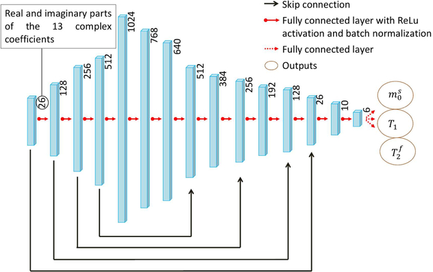
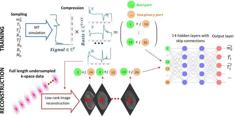
As our quantitative MT model is more complex compared to the Bloch model used in previous NN-based MRF^{18,20,23,19,7}, we use a larger network with more capacity to capture the high-dimensional mapping functions, as shown in Fig. 2. The network size was empirically selected after testing a large span of different architectures to ensure accurate functional mapping while keeping the training time and memory requirements within limits. The network consists of 14 fully-connected layers using systematic experiments to find the hyperparameters defining the architecture with the best performance on testing data. Except for the output layer, each fully-connected layer is followed by group normalization ⁴¹ and rectifier linear units (ReLU) activation functions ⁴². We incorporated skip connections 43 to avoid the vanishing gradient problem during training.

FIGURE 2.

The neural network architecture used in this study. The 13 complex-valued coefficients of each voxel are concatenated and fed into the fully connected network. Skip connections⁴³ are incorporated to avoid the vanishing gradient problem during training. The network outputs the underlying tissue parameters $m_0^s$, T₁ and $T_2^f$, but additional parameters, such as B₀ and B₁, and be added to the output layer (cf. Supporting Information Figure S4).

The network used here treats each voxel independently. The inputs of the network are the 13 complex-valued coefficients of the compressed training or testing data, split into real and imaginary parts and normalized to have an ℓ₂-norm of 1. The outputs of the last layer are the estimated parameters of interest; in our case $m_0^s$, T₁, and $T_2^f$ as we consider these parameters to be the most relevant to our main target application multiple sclerosis and since we optimized the pulse sequence for this purpose 38. The network is, however, also capable of estimating additional parameters, such as _B0 and _B1, with the same training routine and architecture, modified to have more output channels (not shown here).

2.6 |. Training details

The weights of the network are initialized randomly and we used ADAM optimizer⁴⁴ with a batch size of 512. The learning rate was initially set to 0.01 and decayed by half every 40 epochs. We trained the network for 400 epochs, and observed good convergence. We trained two networks: one with proposed CRB-weighted loss (see (1)) and one with the commonly used MSE loss for comparison. We experimentally found this network is not very sensitive to hyper-parameters by searching the hyper-parameter space, therefore, we set them identical when train both networks.

2.7 |. Bias and variance analysis

In order to separate bias from noise in our performance analysis, we process each fingerprint of the two testing datasets with _N different noise realizations for a given SNR_max. This allows us to calculate the bias of a parameter estimate ${\widehat{\theta }}_{p_e,s}$:

$$\mathrm{bias}\left({\theta }_{p_e,s}\right)={\overline{\theta }}_{p_{e,},s}-{\theta }_{p_{e,},S},$$ (2)

as well as the variance

$${\sigma }^2\left({\theta }_{p_e,s}\right)=\sum _{n=1}^N\frac{{\left({\widehat{\theta }}_{n,p_e,s}-{\overline{\theta }}_{p_e,s}\right)}^2}{N}$$ (3)

where n _{∈ {}1_{, … ,N}} runs over all noise realizations, ${\theta }_{p_e,s}$ denotes the ground truth, ${\widehat{\theta }}_{n,p_e,s}$ an estimate, and ${\overline{\theta }}_{p_e,s}$ the average of all N estimates of ${\theta }_{p_e,s}$.

In the same spirit, multiple noise realizations of a single fingerprint allow us to split the average loss of each fingerprint into a bias and a variance component:

$$\begin{gathered} {\overline{L}}_{\text{CRB}}({\theta }_{p_e,s})=\frac{\sum _{n=1}^N{({\widehat{\theta }}_{n,p_e,s}-{\theta }_{p_e,s})}^2}{N\cdot CR{B}_{p_e}({\theta }_{1,s},\dots ,{\theta }_{p_{,s}})} \\ \stackrel{N\to +\infty }{=}\underset{{\overline{L}}_{\text{CRB}}^{\text{bias}}({\theta }_{p_e,s})}{\underbrace{\frac{{({\overline{\theta }}_{p_e,s}-{\theta }_{p_e,s})}^2}{CR{B}_{p_e}({\theta }_{1,s},\dots ,{\theta }_{p_{,s}})}}}+\underset{{\overline{L}}_{\text{CRB}}^{{\sigma }^2}({\theta }_{p_e,s})}{\underbrace{\frac{{\sum }_{n=1}^N{({\widehat{\theta }}_{n,p_e,s}-{\overline{\theta }}_{p_e,s})}^2}{N\cdot CR{B}_{p_e}({\theta }_{1,s},\dots ,{\theta }_{P,s})}}} \end{gathered}$$ (4)

where ${\overline{L}}_{\text{CRB}}^{\text{bias}}({\theta }_{p_e,s})$ and ${\overline{L}}_{\text{CRB}}^{{\sigma }^2}({\theta }_{p_e,s})$ are the contributions of the bias and the variance to the average loss of each parameter and sample ${\theta }_{p_e,s}$, respectively. The bar indicates the loss averaged over multiple noise realizations.

Averaging the loss further over all estimated parameters _pe and samples or fingerprints _s results in the overall loss with its two contributions:

$${\overline{L}}_{\text{CRB}}=\underset{{\overline{L}}_{\text{CRB}}^{\text{bias}}}{\underbrace{\sum _{p_e,s}\frac{{\overline{L}}_{\text{CRB}}^{\text{bias}}({\theta }_{p_e,s})}{P_e\cdot S}}}+\underset{{\overline{L}}_{\text{CRB}}^{{\sigma }^2}}{\underbrace{\sum _{p_e,S}\frac{{\overline{L}}_{\text{CRB}}^{{\sigma }^2}({\theta }_{p_e,s})}{P_e\cdot S}}}.$$ (5)

Note that ${\overline{L}}_{\text{CRB}}={\sum }_n{L}_{\text{CRB},n}/N$ connects this average loss back to the one used during training (Eq. (1)).

We used Eq. (5) to calculate the contributions of bias and variance to the CRB-loss for different SNR_max values by evaluating N _{= 300} noise realizations for each SNR_max. The same analysis was repeated for the MSE-loss without normalizing the CRB values in Eqs. (4). To further investigate those contributions of each parameter to the loss, we conducted this analysis based on each parameter separately for a specific SNR_max.

2.8 |. Phantom and in vivo scans

We built a magnetization transfer phantom with thermally cross-linked bovine serum albumin (BSA). We mixed BSA powder with distilled water in three different concentrations: 10%, 15%, and 20% of the overall sample weight. The mixtures were stirred at 30°C until the BSA was fully dissolved. We split each solution into two batches and doped one of them with 0.1mM MnCl₂. We filled six plastic tubes with the resulting solutions and thermally cross-linked them in a water bath at approximately 90°C for 10 minutes. We note that the 10% BSA mixture without MnCl₂ was cross-linked separately as a trial run, which seemed to have resulted in somewhat inconsistent MT properties. We immersed the six tubes in a head-sized cylindrical container filled with doped water.

We scanned the phantom with our hybrid-state qMT sequence³⁸ on a 3T Prisma scanner (Siemens Healthineers, Erlangen, Germany) with a 20-channel head coil. The qMT sequence drives the magnetization into an anti-periodic transient state by continuously repeating a 4s-long train of flip angles and inverting the magnetization after each cycle. Both, the flip angle and RF-pulse duration are varied to encode the MT parameters. A short TR of 3.5 ms is used to reduce the impact of local variations of the main magnetic field ΔB₀ and to maximize the amount of k-space data sampled throughout the experiment. The sequence acquires 3D data with 1mm isotropic resolution in approximately 12 minutes with a radial koosh-ball k-space trajectory, whose angles are incremented by 2D-golden angles^38,45,46,47.

We further scanned an asymptomatic volunteer with approval of our institutional review board and after getting informed consent. For the in vivo scan, we used a 64-channel head-neck coil and we compressed the data to 20 virtual coils with a singular value decomposition.

Both datasets were reconstructed with the low rank inversion described in Ref.³⁶, using the 13 singular vectors from above described SVD of the training data. We used the BART implementation of this reconstruction ^48,49 and added locally-low rank regularization to reduce undersampling artifacts and noise ⁴⁸. With those reconstruction techniques, the 13 resulting coefficient images show visually minimal undersampling artifacts. In absence of a better statistics of the residual artifacts and noise, we heuristically assume that they are Gaussian distributed and some recent works have found that training neural networks with Gaussian noise was leading to good performance on real data that are known to be corrupted in a non-Gaussian way⁵⁰. Voxel-by-voxel, these 13 complex-valued coefficients, split into real and imaginary parts, and normalized to have an ℓ₂-norm of 1, are fed into the neural networks for the parameter estimation.

To analyze the phantom data, we selected a central slice through the phantom and masked each tube separately. We eroded the out-most voxels to avoid partial-volume effects and performed a box-plot analysis. Thereafter, we compare parameters estimated with a non-linear least square fit (NLLS), with the neural network that was trained with the MSE loss, and with the neural network trained with the CRB-weighted loss.

3 |. RESULTS

3.1 |. Convergence analysis

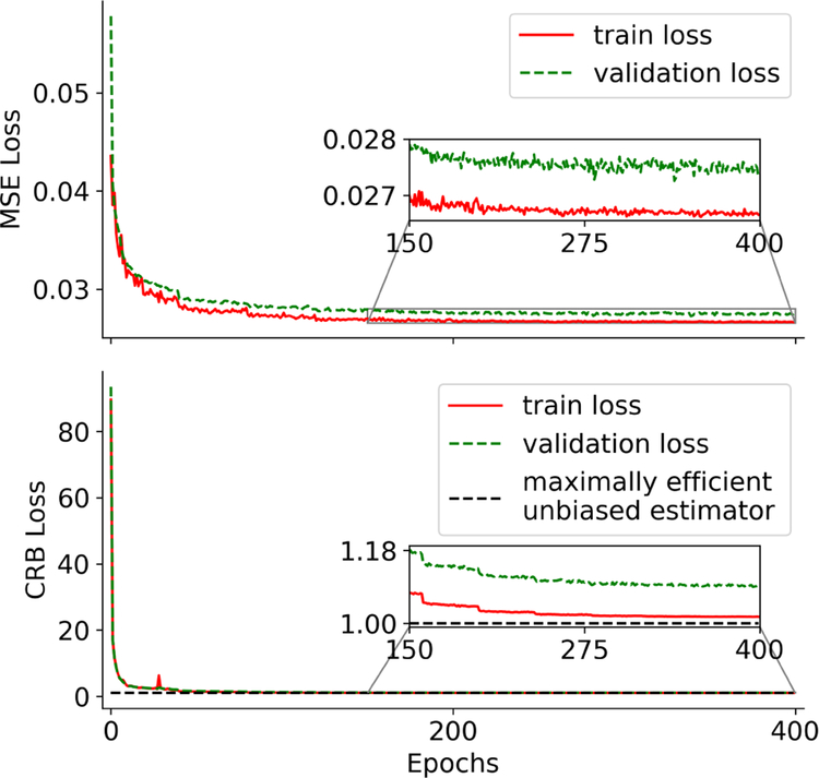
Fig. 3 reveals that the CRB-weighted loss indeed converges approximately to 1, which is a necessary (but not sufficient) condition of a maximally efficient unbiased estimator and, thus, provides an absolute evaluation metric. In contrast, the MSE-loss converges to a value that gives little insight in the performance of the network. Additionally, the CRB-loss converges virtually monotonously while the MSE-loss exhibits comparably strong fluctuations.

FIGURE 3.

Convergence of the training and validation loss. The CRB-loss converges to approximately 1, which corresponds to the loss of a maximally efficient unbiased estimator, while the MSE-loss converges to a value that provides little insight in the performance of the network. The two curves result from separate networks trained with respective loss function.

3.2 |. Bias and variance analysis of the converged networks

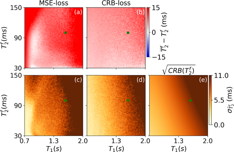
In order to confirm that the network trained with the CRB-loss approximates a maximally efficient unbiased estimator, we performed three analyses. The first one aims at a visual analysis and uses the testing dataset #2 that lies on a regular grid. As the parameter space is 8-dimensional, this analysis is limited to single slices through this space. When using the network trained with the CRB-loss, the bias of the $T_2^f$ estimation in a slice spanned by _T1 and $T_2^f$ is small (Fig. 4b; 5.23ms on average) compared to the bias of the estimation with the MSE-based network (Fig. 4a; 14.1ms on average).

FIGURE 4.

Bias (a,b) and standard deviation (c,d) of $T_2^f$, estimated with the networks trained with the MSE-loss and CRB-loss, respectively. The standard deviation is compared to the square root of the Cramér-Rao bound (e), which provides a theoretical lower bound for an unbiased estimator. The green dots indicate the mean values of the corresponded parameters in the training dataset.The maps were generated with the test dataset #2.

Comparing the standard deviation of estimates to the square root of the Cramér-Rao bound, we observe close concordance in the case of the network trained with the CRB-loss, while we observe substantial deviations for the network trained with the MSE-loss (Fig. 4c–e). In particular at short T₁ and long $T_2^f$ times, the standard deviation of ${\widehat{T}}_2^f$, estimated with the MSE-based network, is substantially larger compared to the square root of the CRB, indicating sub-optimal precision in addition to the large bias (Fig. 4a,c). In contrast, when using the network trained with the CRB loss, we find good agreement between standard deviation of the parameter estimates and the square root of the CRB itself, which indicates that this network approximates a maximally efficient unbiased estimator. Overall, the two networks have similar performance in estimating $m_0^s$ and _T1 on the dataset #2 (cf. Supporting Information), while we do observe a substantial difference in the performance in estimating $T_2^f$.

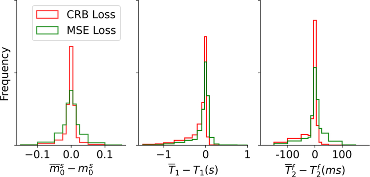
These findings are confirmed by an analysis of the test dataset #1, which covers the same volume in the 8D parameter space as the training data. The bias of $m_0^s$, visualized with histograms in Fig. 5, is overall smaller when using the CRB-based network in comparison to the MSE-based network. The same holds true for _T1 and $T_2^f$, as evident by the higher count in the bin centered around zero bias. This finding is, however, somewhat obscured by the opposite signs in the biases when comparing the two networks.

FIGURE 5.

Bias analysis. The randomly sampled fingerprints in test dataset #1 were processed with 300 noise realizations (SNR_max= ₅₀) and the mean value is compared to the ground truth. Overall, one can observe a smaller bias when estimating the parameters with the network trained with the CRB-loss compared to the network trained with the MSE-loss.

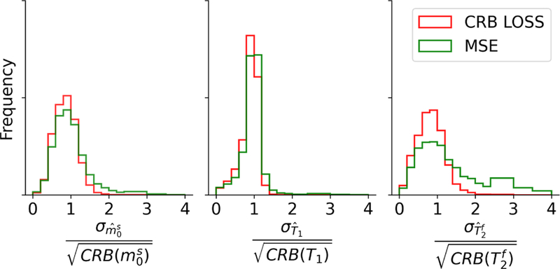
Fig. 6 depicts the ratio of the estimates’ standard deviation and the square root of the CRB. For a maximally efficient unbiased estimator, this ratio is 1 and the network trained with the CRB-loss approximates this property well and better compared to the network trained with the MSE-loss, in particular in the estimation of $T_2^f$.

FIGURE 6.

Standard deviation analysis. The randomly sampled fingerprints in test dataset #1 were processed with 300 noise realizations (SNR_max= 50) and the standard deviation of the estimates is analyzed. Overall, one can observe a smaller variance when estimating the parameters with the CRB-based network compared to the network trained with the MSE-loss. A maximally efficient unbiased estimator has a standard deviation, divided by the square root of the CRB, of 1.

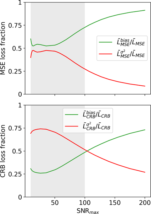
In the third analysis, we decomposed the loss with Eq. (5) into a bias and a variance component. In the case of the MSE-based network, the loss is dominated by the bias. In contrast, the loss of the CRB-based network is dominated by the variance within the training range of SNR_max ∈ [10,100] and the bias component becomes dominant only at SNR_max values outside of the training range (Fig. 7).

FIGURE 7.

Bias and variance contributions to the loss. In case of the network trained with the MSE-loss, the bias dominates the overall loss. In contrast, the loss of the CRB-based network is dominated by the variance within the training range SNR_max ∈ [10,100], highlighted by the gray shade. This decomposition of CRB-loss was performed with Eq. (5) on the test dataset #1.

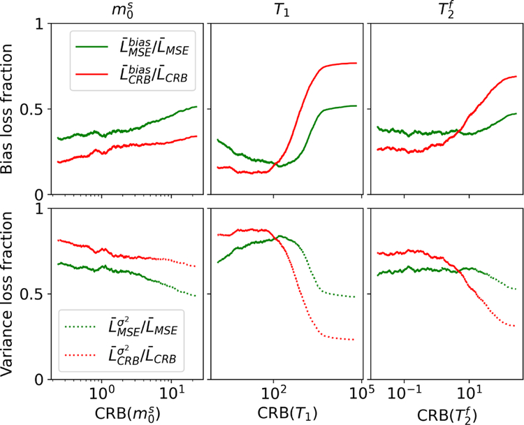
Taking a close look at the loss composition at SNR_max = 50, which is roughly the SNR found in vivo, we find that the bias contributions are overall lower for the CRB-based network, with the exception of _T1 and $T_2^f$ at very high CRB values (Fig. 8). This confirms that, at least for parameter combinations with moderate CRB values, the CRB-based network results on average in a smaller bias.

FIGURE 8.

Bias and variance contributions to the loss. The CRB-based network results overall in a smaller bias compared to the MSE-based network, with the exception of T₁ and $T_2^f$ at very high CRB-values, i.e. for parameter combinations that are hard to estimate. The decompositions of the loss were performed with Eqs. (4) and (5) on the test dataset #1 with SNR_max = 50 and is further split into separate parameters.

3.3 |. Phantom data

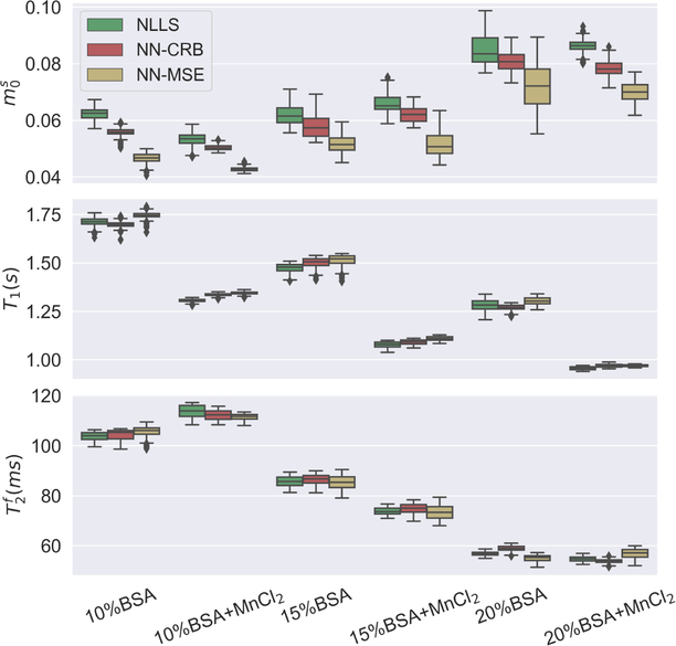
The improved performance of the network trained with the CRB-loss is confirmed by phantom experiments (Fig. 9). We estimated $m_0^s$, T₁, and $T_2^f$ for the samples with different BSA concentrations using the two neural networks, as well as a non-linear least square (NLLS) fitting algorithm, which we consider the gold standard due to its widespread use in quantitative MRI, the lack of an alternative (a brute force dictionary search is unfeasible in 8 dimensions), and despite the risk of it getting stuck in a local minimum. For virtually all samples, we found better agreement of the CRB-based network estimates with the NLLS results, compared to the MSE-based network estimates. For most samples, the estimates with the CRB-based network and the NLLS algorithm match within their interquartile range. The most pronounced deviations can be found in $m_0^s$, which has overall the highest CRB and is, thus, the most difficult one to estimate (not shown here). Estimates calculated with the MSE-based network are overall in good agreement with the NLLS fits as well. Yet, the deviations are somewhat larger compared to the CRB-based network. Further, analyzing the interquartile rangeas well as the overallrange of estimates, we find that the CRB-based network has variations comparable to, and for many samples slightly smaller than the spread of NLLS estimates. In comparison, the spread of the MSE-based network estimates is larger for most samples.

FIGURE 9.

Estimates of $m_0^s$, T₁, and $T_2^f$ from a custom phantom containing different concentrations of thermally cross-linked bovine serum albumin (BSA), half of them doped with MnCl₂. The three methods analyzed here show overall good agreement, but the neural network (NN) trained with the CRB loss is consistently in better agreement with the non-linear least square (NLLS) fits, which we consider the gold standard.

3.4 |. In vivo data

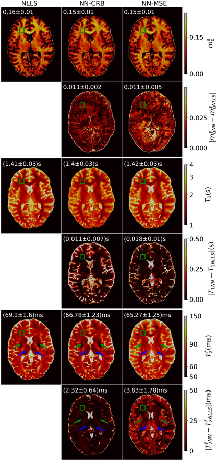
The in vivo data paints largely the same picture: We find overall good agreement between both networks and the NLLS fits. For $m_0^s$, the relative deviations between the CRB-based network and NLLS is approximately 10% and the deviations for the MSE-based network are slightly larger. For the _T1 estimations, the MSE-based network performs slightly better, which is in line with our finding that the MSE training puts more emphasis on _T1.

The biggest difference is observed in the estimates of $T_2^f$, where the CRB-based network performs substantially better compared to the MSE-based network: In the globus pallidus(green arrow in Fig. 10) and the thalamus(blue arrow in Fig. 10), the NLLS and CRB-based network estimations show short $T_2^f$ relaxation times as a result of iron deposition ^51,52. The MSE-based network is not able to capture this signal variation. These findings are also in line with our conceptual and numerical analysis of the networks, which suggested that the MSE-based network performs particularly poorly in $T_2^f$.

FIGURE 10.

A transversal slice through 3D in vivo maps of $m_0^s$, T₁ and $T_2^f$, estimated with non-linear least square (NLLS) fitting, a neural network trained the CRB-loss (NN-CRB) and with the MSE-loss (NN-MSE) respectively. The biggest deviations are observed in $T_2^f$ between MSE-based network estimates and NLLS estimates, which we consider the gold standard. The green arrows point to the globus pallidus and the blue arrows point to the thalamus. The MSE-based network does not capture the short $T_2^f$ relaxation times resulting form the iron deposition in those regions. The green rectangle indicates a frontal white matter region of interest (ROI). The mean and standard deviation of the estimates in this ROI can be found in the top left corner of each subfigure.

4 |. DISCUSSION

As neural networks are increasingly being used to fit biophysical models to MRI data, the need for tailored methods becomes more apparent. Here, we took on the task of finding a training loss that delivers robustness even in heterogeneous parameter spaces. We found that off-the-shelf loss functions like the mean squared error over-emphasize estimates that have large values or naturally have a large error, e.g., because the parameter, at this particular value, is not well encoded by the pulse sequence. The precision with which a parameter is encoded is characterized by the Cramér-Rao bound (CRB) and we demonstrated in this paper that normalizing the squared error of each estimate by respective CRB balances the individual contributions to the training loss.

This normalization of the squared error with the CRB is not entirely heuristic, but rather follows some theoretical concepts: first, it makes the loss of each parameter dimensionless, which allows for adding up the loss of multiple parameters. Second, it normalizes the loss by the one of a maximally efficient unbiased estimator, which provides an absolute evaluation metric for a network; and the networks we trained with the CRB-loss indeed converged approximately to the one of a maximally efficient unbiased estimator.

In order to confirm that our network indeed approximates this ideal condition, we analyzed the bias and the variance of the estimates. We found that the bias of the network trained with the CRB-loss is indeed small (Figs. 4, 5, 7–9) and that the noise variance closely resembles the CRB (Figs. 4 and 6), which indicates that the CRB-based network indeed approximates a maximally-efficient unbiased estimator. Further, we found that this approximation is much better compared to a network that was trained with the MSE-loss.

Here, we tested the CRB-loss function at the example of an 8-parameter magnetization transfer model 38. The theoretical foundation of the proposed loss function gives us reason to believe that it results in superior performance for any model, but the necessity for a well-balanced loss function certainly grows with the heterogeneity of the parameter space or, more precisely, with increasing variations of the Cramér-Rao bound between different parameters and/or throughout the parameter space.

We calculated here the CRB assuming independent and identically distributed Gaussian noise, an assumption that is also implicitly baked into the MSE loss. In order to approximately fulfill this assumption, we reconstructed images into a low rank space spanned by singular vectors of the training data 48,36 and used a combination of parallel imaging^53,54 and locally low rank flavored compressed sensing^55,56,48 to virtually remove the undersampling artifacts. This allows us to train the network with additive Gaussian noise rather than relying on a heuristic noise statistics that emulates undersampling artifacts^19,57.

Another advantage of neural networks over NLLS fitting is the computation time. Once the network is trained, we can fit a 3D volume of a whole brain with 1mm isotropic resolution in about 29s on a single CPU. In contrast, NLLS fitting takes, on average, about 30s per voxel on a single CPU, i.e. it takes about one week for a whole brain volume when using 400 CPUs. Thus, using a NN fitting procedure reduces the processing time to a negligible level compared to the low rank reconstruction, which takes several hours for a 3D scan and using our current, preliminary implementation.

To conclude, we have introduced a theoretically well-founded loss function for deep-learning-based method of parameter estimation in quantitative MRI, and demonstrated its superior performance when compared to the commonly used MSE loss function.

FIGURE 1.

The main work flow of the propose magnetic resonance fingerprinting reconstruction approach. During the training, the MRF signal is simulated for each sampled point in the 8-dimensional parameter space. The signal is then projected from the time domain to a 13-dimensional low-rank subspace with basis functions that are pre-calculated from the training dataset. The complex sub-space data is fed into a 14-layer, fully connected network. To retrieve parameter maps from in vivo scans, the undersampled k-space data is reconstructed directly in the low-rank subspace described above ³⁶. Thereafter, the coefficient images are fed into the trained network voxel by voxel for parameter estimation. In the example application used in this paper, the network estimates $m_0^s$, T₁, $T_2^f$^, but this generalizes to other parameters. E.g., we modified the network also estimate B₀ and B₁.

References

- [1].Barkhof F The clinico-radiological paradox in multiple sclerosis revisited. Current opinion in neurology 2002; 15(3): 239–245. [DOI] [PubMed] [Google Scholar]
- [2].Tofts P Quantitative MRI of the brain: measuring changes caused by disease. John Wiley & Sons. 2005. [Google Scholar]
- [3].Matzat SJ, Tiel vJ, Gold GE, Oei EH. Quantitative MRI techniques of cartilage composition. Quantitative imaging in medicine and surgery 2013; 3(3): 162. [DOI] [PMC free article] [PubMed] [Google Scholar]
- [4].Jelescu IO, Veraart J, Fieremans E, Novikov DS. Degeneracy in model parameter estimation for multi-compartmental diffusion in neuronal tissue. NMR in Biomedicine 2016; 29(1): 33–47. [DOI] [PMC free article] [PubMed] [Google Scholar]
- [5].Ma D, Gulani V, Seiberlich N, et al. Magnetic resonance fingerprinting. Nature 2013; 495(7440): 187–192. [DOI] [PMC free article] [PubMed] [Google Scholar]
- [6].Hamilton JI, Seiberlich N. Machine learning for rapid magnetic resonance fingerprinting tissue property quantification. Proceedings of the IEEE 2019; 108(1): 69–85. [DOI] [PMC free article] [PubMed] [Google Scholar]
- [7].Song P, Eldar YC, Mazor G, Rodrigues MR. HYDRA: Hybrid deep magnetic resonance fingerprinting. Medical physics 2019; 46(11): 4951–4969. [DOI] [PubMed] [Google Scholar]
- [8].Cauley SF, Setsompop K, Ma D, et al. Fast group matching for MR fingerprinting reconstruction. Magnetic resonance in medicine 2015; 74(2): 523–528. [DOI] [PMC free article] [PubMed] [Google Scholar]
- [9].Yang M, Ma D, Jiang Y, et al. Low rank approximation methods for MR fingerprinting with large scale dictionaries. Magnetic resonance in medicine 2018; 79(4): 2392–2400. [DOI] [PMC free article] [PubMed] [Google Scholar]
- [10].Davies M, Puy G, Vandergheynst P, Wiaux Y. A compressed sensing framework for magnetic resonance fingerprinting. Siam journal on imaging sciences 2014; 7(4): 2623–2656. [Google Scholar]
- [11].Mazor G, Weizman L, Tal A, Eldar YC. Low-rank magnetic resonance fingerprinting. Medical physics 2018; 45(9): 4066–4084. [DOI] [PubMed] [Google Scholar]
- [12].Wang Z, Li H, Zhang Q, Yuan J, Wang X. Magnetic resonance fingerprinting with compressed sensing and distance metric learning. Neurocomputing 2016; 174: 560–570. [Google Scholar]
- [13].Boux F, Forbes F, Arbel J, Barbier E. Dictionary-free MR fingerprinting parameter estimation via inverse regression. In: Joint Annual Meeting ISMRM-ESMRMB 2018.; 2018: 1–2. [Google Scholar]
- [14].Nataraj G, Nielsen J, Scott C, Fessler JA. Dictionary-Free MRI PERK: Parameter Estimation via Regression with Kernels. IEEE Transactions on Medical Imaging 2018; 37(9): 2103–2114. [DOI] [PMC free article] [PubMed] [Google Scholar]
- [15].Zhang C, Bengio S, Hardt M, Recht B, Vinyals O. Understanding deep learning (still) requires rethinking generalization. Communications of the ACM 2021; 64(3): 107–115. [Google Scholar]
- [16].Fang Z, Chen Y, Liu M, et al. Deep learning for fast and spatially constrained tissue quantification from highly accelerated data in magnetic resonance fingerprinting. IEEE transactions on medical imaging 2019; 38(10): 2364–2374. [DOI] [PMC free article] [PubMed] [Google Scholar]
- [17].Fang Z, Chen Y, Hung SC, Zhang X, Lin W, Shen D. Submillimeter MR fingerprinting using deep learning–based tissue quantification. Magnetic resonance in medicine 2020; 84(2): 579–591. [DOI] [PMC free article] [PubMed] [Google Scholar]
- [18].Hoppe E, Körzdörfer G, Würfl T, et al. Deep Learning for Magnetic Resonance Fingerprinting: A New Approach for Predicting Quantitative Parameter Values from Time Series. Studies in health technology and informatics 2017; 243. [PubMed] [Google Scholar]
- [19].Virtue P, Stella XY, Lustig M. Better than real: Complex-valued neural nets for MRI fingerprinting. In: 2017 IEEE international conference on image processing (ICIP).; 2017: 3953–3957. [Google Scholar]
- [20].Cohen O, Zhu B, Rosen MS. MR fingerprinting deep reconstruction network (DRONE). Magnetic resonance in medicine 2018; 80(3): 885–894. [DOI] [PMC free article] [PubMed] [Google Scholar]
- [21].Hoppe E, Körzdörfer G, Nittka M, et al. Deep learning for magnetic resonance fingerprinting: Accelerating the reconstruction of quantitative relaxation maps. In: Proceedings of the 26th Annual Meeting of ISMRM, Paris, France.; 2018. [Google Scholar]
- [22].Oksuz I, Cruz G, Clough J, et al. Magnetic resonance fingerprinting using recurrent neural networks. In: 2019 IEEE 16th International Symposium on Biomedical Imaging (ISBI 2019).; 2019: 1537–1540. [Google Scholar]
- [23].Golbabaee M, Chen D, Gómez PA, Menzel MI, Davies ME. Geometry of deep learning for magnetic resonance fingerprinting. In: ICASSP 2019–2019 IEEE International Conference on Acoustics, Speech and Signal Processing (ICASSP).; 2019: 7825–7829. [Google Scholar]
- [24].Balsiger F, Konar AS, Chikop S, et al. Magnetic resonance fingerprinting reconstruction via spatiotemporal convolutional neural networks. In: International Workshop on Machine Learning for Medical Image Reconstruction.; 2018: 39–46. [Google Scholar]
- [25].Hoppe E, Körzdörfer G, Würfl T, et al. Deep Learning for Magnetic Resonance Fingerprinting: A New Approach for Predicting Quantitative Parameter Values from Time Series.. In: GMDS.; 2017: 202–206. [PubMed] [Google Scholar]
- [26].McGivney DF, Pierre E, Ma D, et al. SVD compression for magnetic resonance fingerprinting in the time domain. IEEE transactions on medical imaging 2014; 33(12): 2311–2322. [DOI] [PMC free article] [PubMed] [Google Scholar]
- [27].Gómez PA, Cencini M, Golbabaee M, et al. Rapid three-dimensional multiparametric MRI with quantitative transient-state imaging. Scientific reports 2020; 10: 1–17. [DOI] [PMC free article] [PubMed] [Google Scholar]
- [28].Jones J Optimal sampling strategies for the measurement of relaxation times in proteins. Journal of Magnetic Resonance 1997; 126(2): 283–286. [Google Scholar]
- [29].Jones J, Hodgkinson P, Barker A, Hore P. Optimal sampling strategies for the measurement of spin–spin relaxation times. Journal of Magnetic Resonance, Series B 1996; 113(1): 25–34. [Google Scholar]
- [30].Teixeira RPA, Malik SJ, Hajnal JV. Joint system relaxometry (JSR) and Cramer-Rao lower bound optimization of sequence parameters: a framework for enhanced precision of DESPOT T1 and T2 estimation. Magnetic resonance in medicine 2018; 79(1): 234–245. [DOI] [PMC free article] [PubMed] [Google Scholar]
- [31].Assländer J, Lattanzi R, Sodickson DK, Cloos MA. Optimized quantification of spin relaxation times in the hybrid state. Magnetic Resonance in Medicine 2019; 82(4): 1385–1397. doi: 10.1002/mrm.27819 [DOI] [PMC free article] [PubMed] [Google Scholar]
- [32].Zhao B, Haldar JP, Setsompop K, Wald LL. Optimal experiment design for magnetic resonance fingerprinting. In: 2016 38th Annual International Conference of the IEEE Engineering in Medicine and Biology Society (EMBC).; 2016: 453–456. [DOI] [PMC free article] [PubMed] [Google Scholar]
- [33].Rao CR. Information and the accuracy attainable in the estimation of statistical parameters. In: Springer. 1992. (pp. 235–247). [Google Scholar]
- [34].Cramer H Princeton University Press; Princeton, NJ.. Mathematical Methods of Statistics.[Google Scholar] 1946. [Google Scholar]
- [35].Assländer J, Gultekin C, Flassbeck S, Glaser SJ, Sodickson DK. Generalized Bloch model: a theory for pulsed magnetization transfer. arXiv preprint arXiv:2107.11000 2021. [DOI] [PMC free article] [PubMed] [Google Scholar]
- [36].Assländer J, Cloos MA, Knoll F, Sodickson DK, Hennig J, Lattanzi R. Low rank alternating direction method of multipliers reconstruction for MR fingerprinting. Magnetic resonance in medicine 2018; 79(1): 83–96. [DOI] [PMC free article] [PubMed] [Google Scholar]
- [37].Assländer J, Novikov DS, Lattanzi R, Sodickson DK, Cloos MA. Hybrid-state free precession in nuclear magnetic resonance. Communications Physics 2019; 2(1). doi: 10.1038/s42005-019-0174-0 [DOI] [PMC free article] [PubMed] [Google Scholar]
- [38].Jakob Assländer DKS. Quantitative Magnetization Transfer Imaging in the Hybrid State. In: Proceedings of the 2019 ISMRM and SMRT annual meeting and exhibition.; 2019. [Google Scholar]
- [39].Henkelman RM, Huang X, Xiang QS, Stanisz G, Swanson SD, Bronskill MJ. Quantitative interpretation of magnetization transfer. Magnetic resonance in medicine 1993; 29(6): 759–766. [DOI] [PubMed] [Google Scholar]
- [40].Assländer J A Perspective on MR Fingerprinting. J. Magn. Reson. Imaging 2021; 53(3): 676–685. doi: 10.1002/jmri.27134 [DOI] [PMC free article] [PubMed] [Google Scholar]
- [41].Wu Y, He K. Group normalization. In: Proceedings of the European conference on computer vision (ECCV).; 2018: 3–19. [Google Scholar]
- [42].Agarap AF. Deep learning using rectified linear units (relu). arXiv preprint arXiv:1803.08375 2018. [Google Scholar]
- [43].He K, Zhang X, Ren S, Sun J. Deep residual learning for image recognition. In: Proceedings of the IEEE conference on computer vision and pattern recognition.; 2016: 770–778. [Google Scholar]
- [44].Kingma DP, Ba J. Adam: A method for stochastic optimization. arXiv preprint arXiv:1412.6980 2014. [Google Scholar]
- [45].Flassbeck S, Assländer J. Minimization of Eddy Current Related Artefacts in Hybrid-State Sequences. In: Proceedings of the 2021 ISMRM and SMRT annual meeting and exhibition.; 2021. [Google Scholar]
- [46].Winkelmann S, Schaeffter T, Koehler T, Eggers H, Doessel O. An optimal radial profile order based on the Golden Ratio for time-resolved MRI. IEEE transactions on medical imaging 2006; 26(1): 68–76. [DOI] [PubMed] [Google Scholar]
- [47].Chan RW, Ramsay EA, Cunningham CH, Plewes DB. Temporal stability of adaptive 3D radial MRI using multidimensional golden means. Magnetic Resonance in Medicine: An Official Journal of the International Society for Magnetic Resonance in Medicine 2009; 61(2): 354–363. [DOI] [PubMed] [Google Scholar]
- [48].Tamir JI, Uecker M, Chen W, et al. T2 shuffling: sharp, multicontrast, volumetric fast spin-echo imaging. Magnetic resonance in medicine 2017; 77(1): 180–195. [DOI] [PMC free article] [PubMed] [Google Scholar]
- [49].Uecker M, Tamir JI, Ong F, Lustig M. The BART toolbox for computational magnetic resonance imaging. ISMRM: Concord, CA, USA: 2016. [Google Scholar]
- [50].George D, Huerta EA. Deep Learning for real-time gravitational wave detection and parameter estimation: Results with Advanced LIGO data. Physics Letters B 2018; 778: 64–70. [Google Scholar]
- [51].Péran P, Cherubini A, Luccichenti G, et al. Volume and iron content in basal ganglia and thalamus. Human brain mapping 2009; 30(8): 2667–2675. [DOI] [PMC free article] [PubMed] [Google Scholar]
- [52].Walsh AJ, Blevins G, Lebel RM, Seres P, Emery DJ, Wilman AH. Longitudinal MR imaging of iron in multiple sclerosis: an imaging marker of disease. Radiology 2014; 270(1): 186–196. [DOI] [PubMed] [Google Scholar]
- [53].Sodickson DK, Manning WJ. Simultaneous acquisition of spatial harmonics (SMASH): fast imaging with radiofrequency coil arrays. Magnetic resonance in medicine 1997; 38(4): 591–603. [DOI] [PubMed] [Google Scholar]
- [54].Pruessmann KP, Weiger M, Börnert P, Boesiger P. Advances in sensitivity encoding with arbitrary k-space trajectories. Magnetic Resonance in Medicine: An Official Journal of the International Society for Magnetic Resonance in Medicine 2001; 46(4): 638–651. [DOI] [PubMed] [Google Scholar]
- [55].Lustig M, Donoho DL, Santos JM, Pauly JM. Compressed sensing MRI. IEEE signal processing magazine 2008; 25(2): 72–82. [Google Scholar]
- [56].Trzasko J, Manduca A. Local versus global low-rank promotion in dynamic MRI series reconstruction. In: Proceedings of the 19th Annual Meeting of ISMRM,Montreal, Canada.; 2011. [Google Scholar]
- [57].Virtue P, Tamir JI, Doneva M, Yu SX, Lustig M. Learning contrast synthesis from MR fingerprinting. In: Proc. 26th Annu. Meeting (ISMRM). icsi. berkeley. edu.; 2018: 676. [Google Scholar]
Associated Data
This section collects any data citations, data availability statements, or supplementary materials included in this article.