A multi-scale map of cell structure fusing protein images and interactions

Abstract

The cell is a multi-scale structure with modular organization across at least four orders of magnitude¹. Two central approaches for mapping this structure—protein fluorescent imaging and protein biophysical association—each generate extensive datasets, but of distinct qualities and resolutions that are typically treated separately^2,3. Here we integrate immunofluorescence images in the Human Protein Atlas⁴ with affinity purifications in BioPlex⁵ to create a unified hierarchical map of human cell architecture. Integration is achieved by configuring each approach as a general measure of protein distance, then calibrating the two measures using machine learning. The map, known as the multi-scale integrated cell (MuSIC 1.0), resolves 69 subcellular systems, of which approximately half are to our knowledge undocumented. Accordingly, we perform 134 additional affinity purifications and validate subunit associations for the majority of systems. The map reveals a pre-ribosomal RNA processing assembly and accessory factors, which we show govern rRNA maturation, and functional roles for SRRM1 and FAM120C in chromatin and RPS3A in splicing. By integration across scales, MuSIC increases the resolution of imaging while giving protein interactions a spatial dimension, paving the way to incorporate diverse types of data in proteome-wide cell maps.

Eukaryotic cells consist of large components, such as organelles, which recursively factor into smaller components, such as condensates and protein complexes, forming an intricate multi-scale structure⁶. Fundamental techniques for mapping subcellular structure are protein imaging and biophysical association, each of which has been extensively automated. In particular, advances in confocal microscopy and immunofluorescence have made it possible to scan the distribution of proteins in situ within single cells². By combining these techniques with a library of antibodies, the Human Protein Atlas (HPA) has embarked on systematic studies to position human proteins into subcellular compartments⁴. As a parallel approach to cell mapping, mass spectrometry (MS) has been powerfully combined with affinity purification (AP–MS) and proximity-dependent labelling to enable rapid measurement of protein–protein associations³. Using AP–MS, the BioPlex project is generating comprehensive interaction maps for most human proteins⁵.

Given these efforts, akey question is how imaging and biophysical association should be combined to inform cell structure. We reasoned that the two platforms provide complementary measures of protein location, albeit of vastly different characters. Images position proteins relative to cellular landmarks such as the nucleus, whereas biophysical associations position proteins relative to nearby proteins. In both cases, such positioning has become increasingly quantitative due, in part, to the ability of machine learning systems to recognize complex patterns in data^7,8.

Here we demonstrate a machine learning approach in which protein imaging and biophysical association are integrated to create a unified map of subcellular components (Fig. 1). First, we use neural networks to project proteins into a small number of dimensions on the basis of imaging or biophysical association. Once protein coordinates have been determined for each platform, pairwise distances among proteins are calibrated and combined to reveal assemblies at different scales, from the very small (less than 50 nm) to the very large (more than 1 µm).

Fig. 1 |. Overview of data fusion strategy.

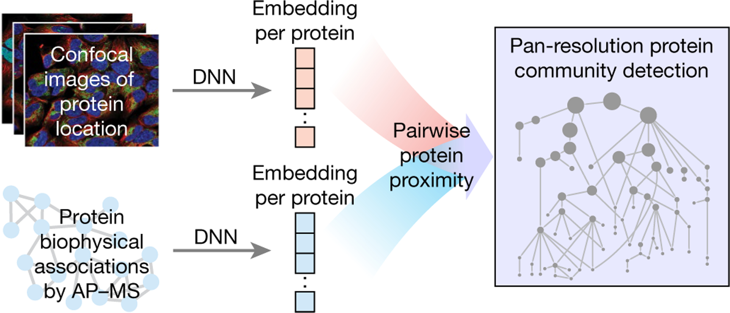
Protein images and interaction data are analysed to generate neural network embeddings for each protein. These embeddings reveal communities of proximal proteins at multiple resolutions to create a multi-scale integrated map of the cell. DNN, deep neural network.

Protein position and distance in two ways

We assembled a matched dataset of immunofluorescence images from HPA⁴ and AP–MS data from BioPlex⁵. Both resources are partially based on human embryonic kidney (HEK293-derived) cells, yielding 661 proteins with compatible imaging (1,451 images including replicates) (Extended Data Fig. 1a–c) and biophysical association data (291 proteins affinity-tagged as ‘baits’, 370 as interacting ‘preys’) (Supplementary Table 1). These proteins covered a wide distribution of subcellular locations similar to that seen for all human proteins (Extended Data Fig. 1d). Other proteins in HPA and BioPlex were measured in differing cell types that did not align; thus, we focused on the common HEK293-derived context for prototyping our approach.

We next used deep neural networks to embed each protein on the basis of its immunofluorescence and AP–MS data. An embedding is a low-dimensional representation of a complex input, in which each data point (here a protein) is assigned coordinates in the reduced dimensions. Much machine learning research has focused on creating a good embedding, in which similar inputs (here proteins with similar subcellular distributions or interactions) are close in the embedded space⁹. For image embedding we used DenseNet⁷, a convolutional neural network with superior performance in capturing protein locations relative to counter-stained cellular landmarks (Extended Data Fig. 2a–c). Similarly, the node2vec neural network⁸ was used to embed each protein using its extended AP–MS interaction neighbourhood (Extended Data Fig. 2d–g).

We then computed protein–protein distances for all protein pairs, separately in immunofluorescence and AP–MS embeddings. The closest pairs measured by one technique were enriched for pairs close in the other, showing that imaging and AP–MS share substantial information (Extended Data Fig. 3a, b). To calibrate distances in the embeddings to physical distances in cells, we assembled a reference set of subcellular components with known or estimated diameters, from protein complexes of less than 20 nm to organelles of more than 1 µm (Extended Data Fig. 3c, Supplementary Table 2, Supplementary Methods). With these curated diameters as training labels, we taught a supervised machine learning model (random forest regression) to estimate the distance of any protein pair directly from its coordinates in the immunofluorescence and AP–MS embeddings (Extended Data Fig. 3d, e).

A multi-scale map of subcellular systems

We analysed all distances among the 661 proteins to identify communities of proteins in close mutual proximity, suggesting distinct components (Fig. 2). Communities were identified at multiple resolutions, starting with those that form at the smallest protein–protein distances, then progressively relaxing the distance threshold (multi-scale community detection¹⁰Extended Data Fig. 4a, Supplementary Methods). Communities at smaller distances were contained, in full or part, inside larger communities as the threshold was relaxed, yielding a structural hierarchy (Fig. 3a). The sensitivity of community detection was tuned for best concordance with two independent datasets: protein interactions reported in the Human Cell Map¹¹ using proximity biotinylation, also in HEK293 cells; and patterns of gene co-essentiality in the Cancer Cell Dependency Map¹². Significant agreement with independent data-sets was observed for a wide range of community detection parameters and for both small and large communities (Extended Data Fig. 4b, e). The final hierarchy, MuSIC 1.0, contained 69 protein communities representing putative subcellular systems organized by 87 hierarchical containment relationships (Fig. 2, Supplementary Table 3). Sixteen systems were contained within multiple larger ones, suggesting multiple subcellular locations or pleiotropy. Approximately 46% had a substantial overlap with cellular components documented in Gene Ontology; we annotated the remaining 54% as putatively novel (Fig. 2).

Fig. 2 |. The multi-scale integrated cell.

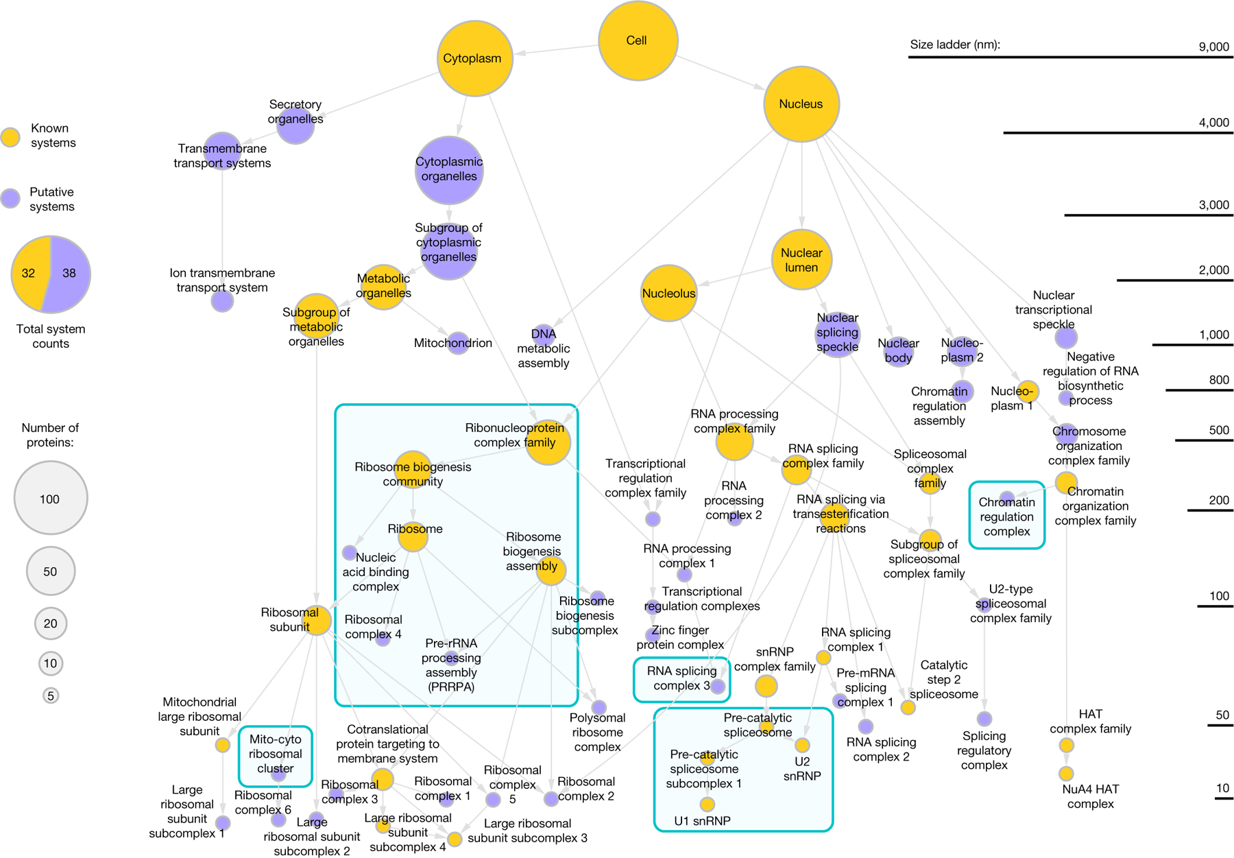
Nodes indicate systems; arrows indicate containment of lower system by upper. Node size, number of system proteins. Node colour, known (gold) versus novel (purple). Teal boxes denote systems detailed in the text and figures. Elevation of system (size ladder) determined by predicted diameter.

Fig. 3 |. MuSIC captures subcellular components and diameters.

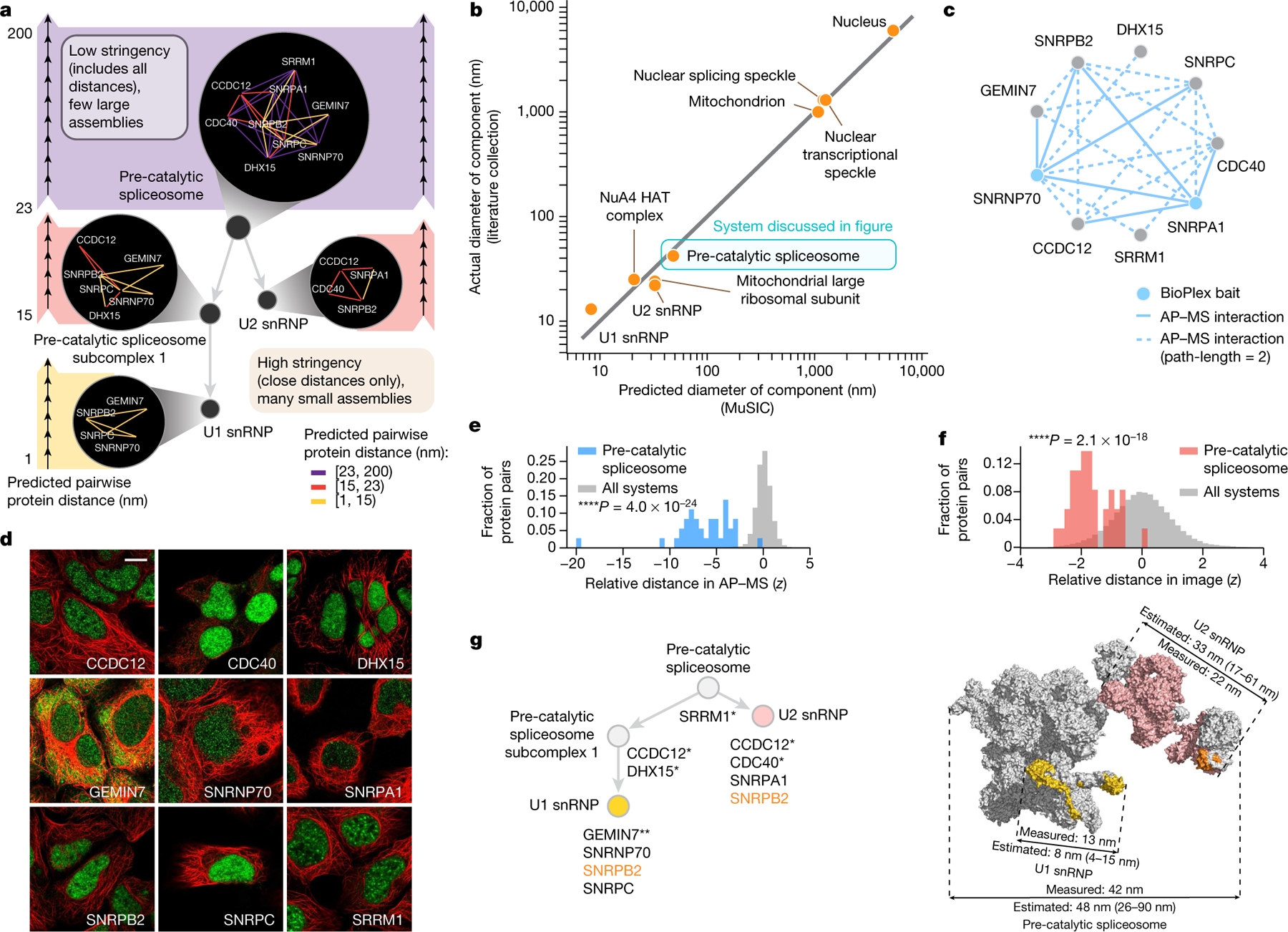
a, Hierarchical community detection. As distance threshold increases (bottom to top), strong communities (systems) are detected first, then expanded to include moderate-to-weak associations. Dark circles, systems; edge colours, association stringency. b, Predicted versus actual diameter of components detailed in literature and not used for calibration. c, Biophysical interaction data for pre-catalytic spliceosome. AP–MS interaction (path-length = 2) indicates protein pairs that interact with common affinity-tagged bait(s) outside the complex. d, Same proteins immunostained (green) with cytoskeleton counterstain (red). Scale bar, 10 µm. e, Histogram of protein–protein distances in AP–MS embedding (z-scores). Blue, pre-catalytic spliceosome; grey, all protein pairs. One-sided Mann–Whitney U test. f, As in e for image rather than AP–MS data. Red, pre-catalytic spliceosome; grey, all protein pairs. g, Hierarchy of spliceosome systems in MuSIC (left) versus 3D structural model (right; Protein Data Bank 6QX9¹⁴). * indicates a pre-catalytic spliceosome protein¹³ captured by MuSIC but not included in structural model; ** indicates a protein important for small nuclear ribonucleoprotein (snRNP) assembly. Proteins are assigned the same colours in both maps. SNRPB2 (orange) is in both U1 and U2 subunits in MuSIC, as suggested previously³⁰; the structural model places it in U2 only.

Physical sizes of MuSIC systems were estimated from their pairwise protein distances (Fig. 2) and compared to known diameters of nine well-characterized cellular components not used earlier in calibration (Fig. 3b, Supplementary Table 4). One of these was the pre-catalytic spliceosome, for which support from both immunofluorescence and AP–MS data (Fig. 3c–f) had induced a protein community of 48 nm (95% prediction interval [26, 90]), in agreement with its published diameter of 42 nm^13,14 (Fig. 3a, g). Within this community, the analysis resolved smaller U1 and U2 subunits (U1: 8 nm, 95% prediction interval [4, 15]; U2: 33 nm, 95% prediction interval [17, 61]), again in agreement with the arrangement and distances measured by cryo-electron microscopy (Fig. 3g). For all nine components, estimated diameters were very close to actual measurements from the literature (Fig. 3b), validating that MuSIC captures and sizes biological systems across a wide range of scales.

MuSIC needs and informs both data types

We found that the majority of systems were robust to minor disruptions in data (Fig. 4a, jackknife resampling, Supplementary Methods). By contrast, alternative MuSIC maps constructed with only one data type dropped numerous systems. Immunofluorescence-only maps tended to identify large systems such as organelles but falter for small subcomponents such as protein complexes, whereas AP–MS maps had the opposite behaviour (Fig. 4b–d). Notably, 30% of AP–MS interactions fell within focused systems of fewer than 100 proteins (Fig. 4e), validating and providing location context for the interaction. Such context also increases the sensitivity of interaction detection: focusing on protein pairs not reported to interact in the previous BioPlex study⁵, pairs in smaller systems nonetheless had stronger AP–MS scores than pairs in larger systems (P < 0.0001; Fig. 4f), suggesting new bona fide physical interactions.

Fig. 4 |. Different data informs different scales of information.

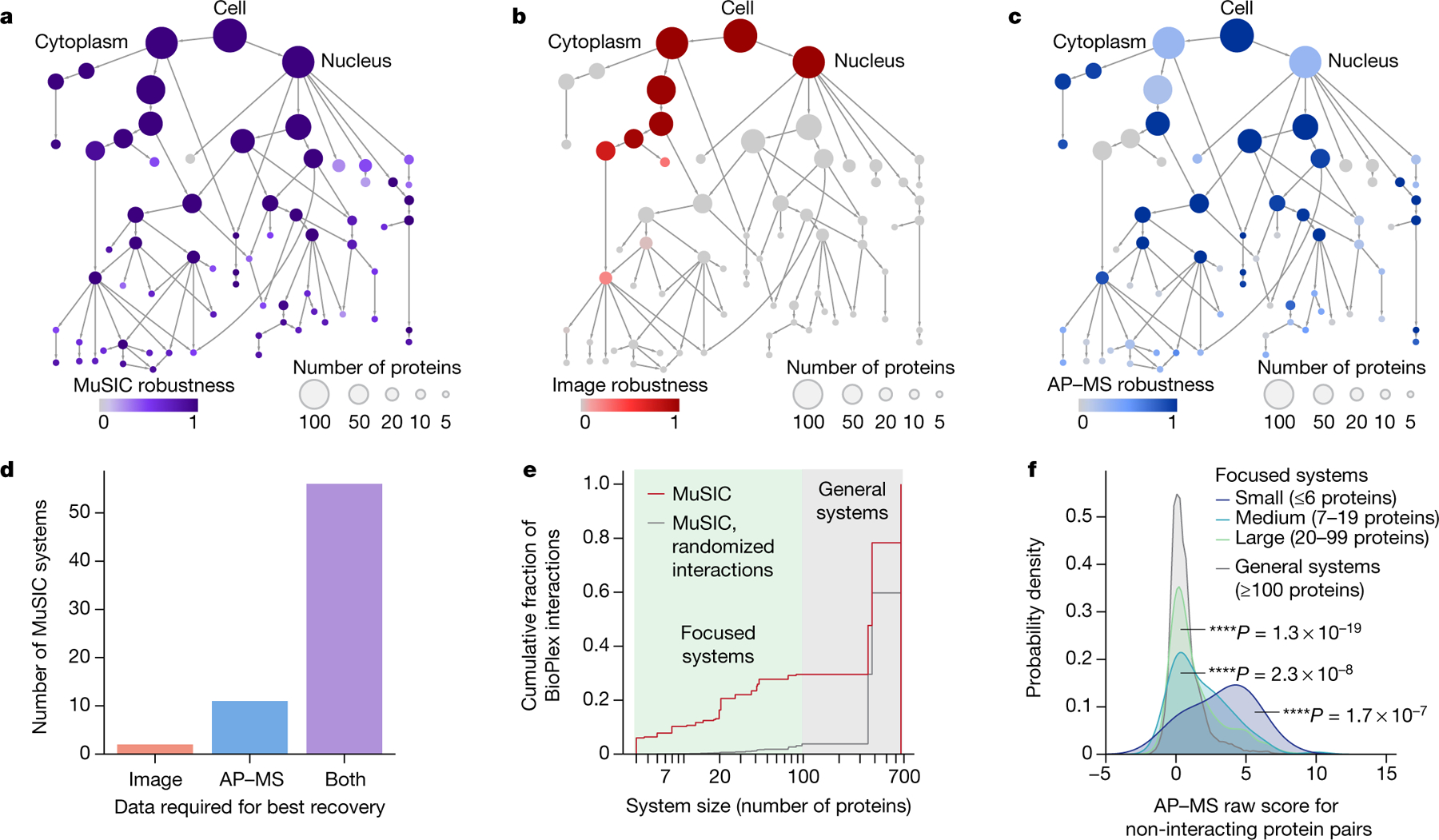
a–c, MuSIC map from Fig. 2, coloured with system robustness when built using imaging and AP–MS data (full MuSIC (a)), imaging only (b) or AP–MS only (c). d, Number of systems for which highest robustness comes with imaging, AP–MS or both types. e, Cumulative fraction of AP–MS interactions within MuSIC systems (red) versus random protein pairs (grey; 1,000 randomizations). f, Distribution of AP–MS scores for protein pairs not labelled as interacting by BioPlex. P values calculated against general systems (at least 100 proteins); one-sided Mann–Whitney U test.

Global validation of MuSIC by new AP–MS

Of the 661 MuSIC proteins, 370 had not yet been affinity-tagged as baits in AP–MS experiments. Rather, they had appeared in the list of prey proteins isolated by another affinity-tagged protein. As an immediate means of validating candidate systems, we affinity-tagged 134 former prey proteins and performed AP–MS, resulting in the identification of 339 physical interactions (Supplementary Table 1). Forty-four MuSIC systems were specifically enriched for new interactions (64%; false discovery rate (FDR) < 0.1) (Fig. 5a), including 23 putative candidates.

Fig. 5 |. Exploration of MuSIC using physical and functional assays.

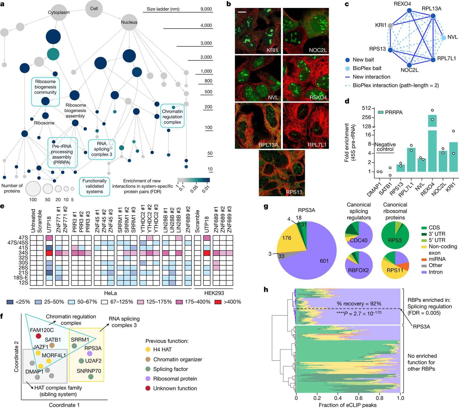
a, Map from Fig. 2 with system colour showing enrichment for new AP–MS interactions (blue gradient, FDR). b, c, Images (b) and AP–MS interactions (c) for PRRPA proteins, displayed as in Fig. 3c, d. Scale bar, 10 µm (b). d, Enrichment of 45S pre-rRNA bound by FLAG–HA-tagged proteins (x axis), measured using RIP–qPCR normalized to DMAP1 (n = 2 stable cell lines). e, Heat map summarizing northern blot analysis of intermediate RNA products during pre-rRNA processing (rows), under DsiRNAs targeting candidate genes (columns). Heat map colour shows the percentage of pre-rRNA versus non-targeting scramble silencer control. UTP18 is a known ribosome biogenesis positive control. Independent silencers (#1–3) were highly consistent. f, Two-dimensional projection (spring embedding) of distances among proteins in chromatin regulation and splicing complexes. g, Pie charts categorize significant eCLIP peaks by genomic region (coloured slices). CDS, coding sequence; miRNA, microRNA; UTR, untranslated region. h, Clustering of RPS3A eCLIP profile (dashed line) with 223 eCLIP profiles²⁵. Proteins robustly clustering with RPS3A (1,000 jackknife resamplings) enrich for splicing regulators (hypergeometric test, Benjamini–Hochberg correction). Colour consistent with g. RBP, RNA-binding protein.

Ribosomal systems at multiple scales

Among candidates validated by the additional AP–MS data was a seven-protein assembly with an estimated diameter of 81 nm (95% prediction interval [43, 151]). We tentatively named this system ‘pre-ribosomal RNA processing assembly’ (PRRPA) on the basis of established pre-rRNA roles for two of its proteins^15,16 (NVL, RPL13A), support from genetic screens¹⁷ (KRI1, NOC2L) and orthology to a pre-rRNA factor in yeast¹⁸ (REXO4). These proteins formed a system due to image similarity, with nucleolar localizations, and similarity of AP–MS network neighbourhoods (Fig. 5b, c, Extended Data Fig. 5a). Our new affinity purifications targeted five PRRPA proteins, and recovered interacting partners highly specific to this system (Fig. 5c, Extended Data Fig. 5b). To explore the function of PRRPA in pre-rRNA processing, we used small interfering RNAs (siRNAs) to knock down each protein; all knockdowns perturbed ribosomal RNA maturation to some extent (Extended Data Fig. 5c–i). We then used RNA immunoprecipitation and quantitative PCR (RIP–qPCR) to find that these proteins bind 45S pre-rRNA, again supporting a pre-rRNA processing role (Fig. 5d).

We also examined the larger-scale system containing PRRPA, ‘ribosome biogenesis community’ (347 nm, 95% prediction interval [186, 646]). This system contained additional proteins not associated with ribosome biogenesis (Extended Data Fig. 6a), seven of which we knocked down with targeted Dicer-substrate siRNAs (DsiRNAs). All seven had effects on pre-rRNA processing, stratified by the specific pre-rRNA affected (Fig. 5e, Extended Data Fig. 6b, c). Three of these proteins were targeted in our new AP–MS experiments (LIN28B, PRR3, ZNF689); each was shown to bind a substantial number of proteins within this same community (Extended Data Fig. 6d).

Another notable finding within ribosomal systems was abundant cross-talk between cytoplasmic and mitochondrial ribosomes (‘mito-cyto ribosomal cluster’; 20 nm, 95% prediction interval [11, 38]) (Extended Data Fig. 6e–h). Several of these proteins were tagged in the new AP–MS experiments (two cytoribosomal, two mitoribosomal), recovering four new physical interactions between cytoplasmic and mitochondrial factors (Extended Data Fig. 6i). Such cross-talk may have a role in mitoribosome biogenesis, a poorly understood process¹⁹.

Chromatin and splicing

SRRM1 is an established splicing factor²⁰ that, in addition to its canonical placement in ‘RNA splicing complex 3’ (71 nm, 95% prediction interval [38, 133]), participated in additional systems that were unexpected. ‘Chromatin regulation complex’ (211 nm, 95% prediction interval [113, 393]) included three histone acetyltransferases (HATs) (DMAP1, JAZF1 and MORF4L1²¹) and SATB1, which remodels chromatin through HAT recruitment²² (Fig. 5f, Extended Data Fig. 7a, b). These functions suggested that SRRM1 and FAM120C, the remaining proteins in this system, also regulate chromatin. In support of this, we found that SRRM1 and FAM120C strongly associate with chromatin by in situ fractionation (Extended Data Fig. 7c).

Returning to RNA splicing complex 3, this system brought SRRM1 and other splicing factors (SNRNP70²³, U2AF2²⁴) together with a ribosomal protein that was not previously associated with major RNA splicing (RPS3A²¹) (Extended Data Fig. 7d, e). However, analysis of published transcriptomic profiles²⁵ indicated that knockdown of RPS3A had very similar transcriptional effects to knockdown of these splicing factors (Extended Data Fig. 7f, g). To test for a role in splicing, we subjected RPS3A to an enhanced ultraviolet cross-linking and immunoprecipitation assay²⁶ (eCLIP, Extended Data Fig. 7h), which identifies and characterizes RNA transcripts bound by a protein. Indeed, RPS3A bound to many intronic RNA sequences (601 eCLIP peaks) (Supplementary Table 5) with a pattern very similar to that of canonical splicing regulators (Fig. 5g). Moreover, when clustering the RPS3A profile with 223 eCLIP profiles from the public domain²⁵, RPS3A robustly clustered with canonical splicing regulators (92% recovery in jackknife resampling) (Fig. 5h), providing further support for an alternative role of this protein in splicing regulation.

Discussion

In classical image analysis, protein proximity is measured by fluorescently labelling multiple proteins in the same image²⁷, a combinatorial process that is difficult to scale. Here we have developed a systematic means of measuring proximity through neural network embeddings of each protein. In turn, systematic accumulation of protein proximities moves us from a fixed list of predefined subcellular components to an open approach in which components are defined by inherent structure in the imaging data. Such analysis also integrates with other types of information, demonstrated here with AP–MS, and recovers components at multiple scales (Fig. 3b), including novel systems that can be physically and functionally validated (Fig. 5). Although imaging research is accustomed to thinking about physical sizes and intracellular distances, the notion that protein interactions provide a complementary measure of intracellular distance is, to our knowledge, new to this study.

Although nearly a third of AP–MS interactions link proteins within a focused system of fewer than 100 proteins, more than two thirds do not (Fig. 4e, Extended Data Fig. 8a). Such discrepancies may indicate transient protein interactions. Alternatively, discrepancies might derive from errors or biases, such as the fact that immunofluorescence detects endogenous proteins whereas AP–MS detects overexpressed tagged proteins. Some disagreement between data types can be tolerated, such as the correct assignment of GEMIN7 and SNRNP70 to the U1 snRNP (Fig. 3g), despite only a partial overlap in their images (Extended Data Fig. 8b). Here, correct assignment was facilitated by physical interaction from AP–MS.

Systems in MuSIC reside at multiple scales, bridging and exceeding the ranges of immunofluorescence and AP–MS (Fig. 4a–d). Here the scale of a component is determined by the estimated nanometre proximities among its members; this measurement of scale only partially correlates with the component’s number of proteins. Analysis of protein proximities at broad scale identified the pre-catalytic spliceosome, whereas decreasing the distance threshold recovered smaller sub-components, the U1 and U2 snRNPs (Fig. 3a, g). As physical proximity increases, one would expect the same for functional association. To this point, gene co-essentiality—a measure of joint function²⁸—was strongest among genes in the same small systems, weaker within larger systems that contain them and near zero for unrelated genes (Extended Data Fig. 8c, d). Components at different scales map naturally to different types of assays for functional exploration. For example, we used 28S/18S rRNA ratio as a general readout affected by proteins in the ribosome biogenesis community. More specific probes implicated specific subfunctions, such as the binding of a protein to 45S pre-rRNA (suggesting early-stage ribosome biogenesis) (Fig. 5d) or changes in 34S pre-rRNA that result from protein knockdown (suggesting maturation defect associated with small-subunit processome¹⁷) (Fig. 5e). We expect future validation of MuSIC systems to draw from a range of functional assays at the molecular, pathway and cellular level.

As the map is developed to cover all human proteins, key questions relate to cellular heterogeneity and dynamics; for example, whether it is preferable to work towards a unified map of subcellular components or to create separate maps cataloguing different cell types and states. An attractive middle road may be to create a small library of reference maps for major cell types, with context-specific differences indicated as annotations. Here, we focused on HEK293-derived cells, a widely used model for gaining general biological insights^4,5,11. Previous studies have shown that approximately 70% of proteins have consistent localization across cell lines⁴ and about 50% maintain their physical interactions²⁹; thus, we expect that the current map will partially generalize to other contexts, with attention paid to communities prone to dynamics. Notably, the proteins of many MuSIC systems are co-regulated in expression across diverse cell types (Extended Data Fig. 8e), suggesting that these systems are indeed relevant to other contexts.

Finally, we note the synergy achieved in integrating HPA and BioPlex, two large-scale mapping efforts that might have progressed independently. Such coordination should continue and encompass collaborative dataset design; for instance, by adopting common cell lines and proteins targeted across projects. Furthermore, new protein systems might arise with the inclusion of additional data modalities, such as proximity-dependent labelling, cross-linking mass spectrometry or cryo-electron microscopy. It will be interesting to explore synergies among these platforms, all of which might be calibrated to measure molecular distances and, in turn, contribute to maps of the multi-scale cell.

Extended Data

Extended Data Fig. 1 |. Characterization of image data used in this study.

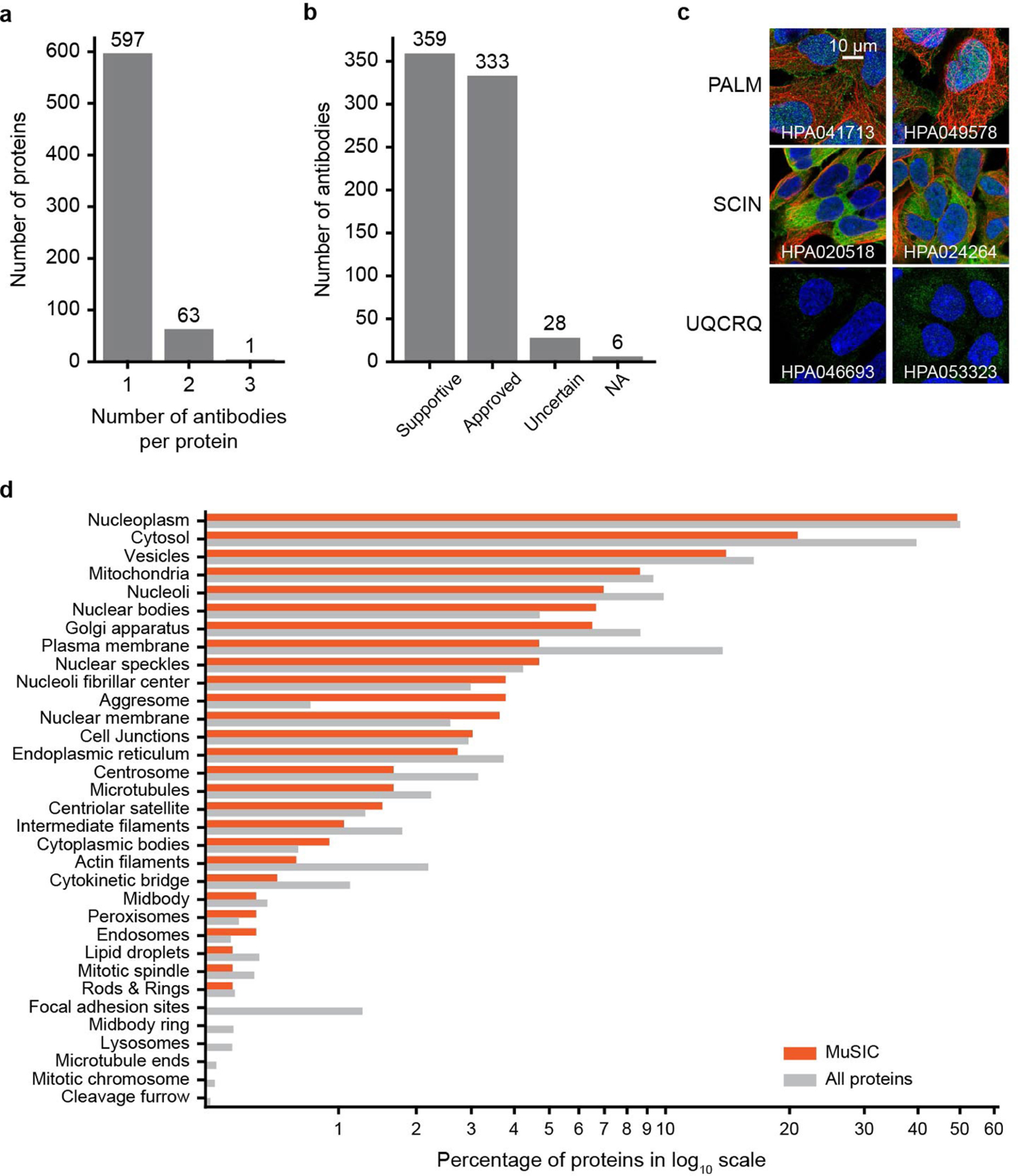
a, Histogram showing distribution in number of antibodies per protein over 661 proteins included in MuSIC. b, Histogram showing distribution in antibody quality scores over antibodies used in this study. c, Immunofluorescence images for alternative antibodies (columns) targeting the same protein (rows). Colours represent immunostained protein (green), cytoskeleton (red), or nucleus (blue). Images show high reproducibility for different antibodies against the same protein. d, Comparison of localizations for proteins in MuSIC (HEK293 cells, red) versus all proteins assayed by HPA in any cell line (grey). Localizations as defined by the HPA project⁴.

Extended Data Fig. 2 |. Embedding immunofluorescence images and AP–MS data.

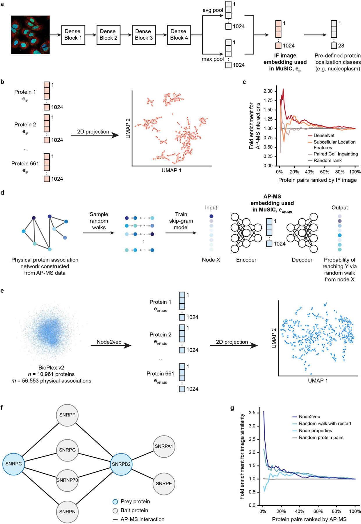
a, Embedding immunofluorescence (IF) images using DenseNet. The 1024-dimension feature vector for each IF image was extracted from a DenseNet-121³¹ model trained to classify the IF image into one or several of 28 pre-defined protein localization classes from HPA. b, Two-dimensional visualization (UMAP, n_neighbours = 5) for the 1,451 image embeddings associated with the 661 proteins in MuSIC. c, Ability of different image embedding methods (coloured curves) to generate image-image similarities (cosine similarity) in agreement with protein-protein interactions in BioPlex 2.0. d, Node2vec⁸ workflow. The feature vector generated by node2vec captures the pattern of interaction neighbourhood for the respective node in input network. e, Embedding AP–MS data using node2vec. The input network to node2vec was constructed by treating each protein as a node and assigning edges between protein pairs that were identified as physically interacting in the AP–MS data. The two-dimensional visualization (UMAP, n_neighbours = 5) for AP–MS embeddings associated with 661 proteins in MuSIC is shown at right. f, Network showing all proteins (grey) that physically interact with SNRPC and SNRPB2 (blue) in BioPlex 2.0. SNRPC and SNRPB2 do not physically interact, but the cosine similarity of their embedded features is 0.93 due to shared interaction neighbourhood. In many cases of two proteins with high node2vec similarity but without direct interaction in AP–MS data, we found that neither protein had yet been tagged as bait for an affinity purification experiment. In these cases, the node2vec embedding suggests gaps in existing AP–MS data. g, Ability of different AP–MS embedding methods to generate protein-protein similarities (cosine similarity) in agreement with protein pairwise similarities computed from HPA images.

Extended Data Fig. 3 |. Fusing protein distances from immunofluorescence and affinity purification.

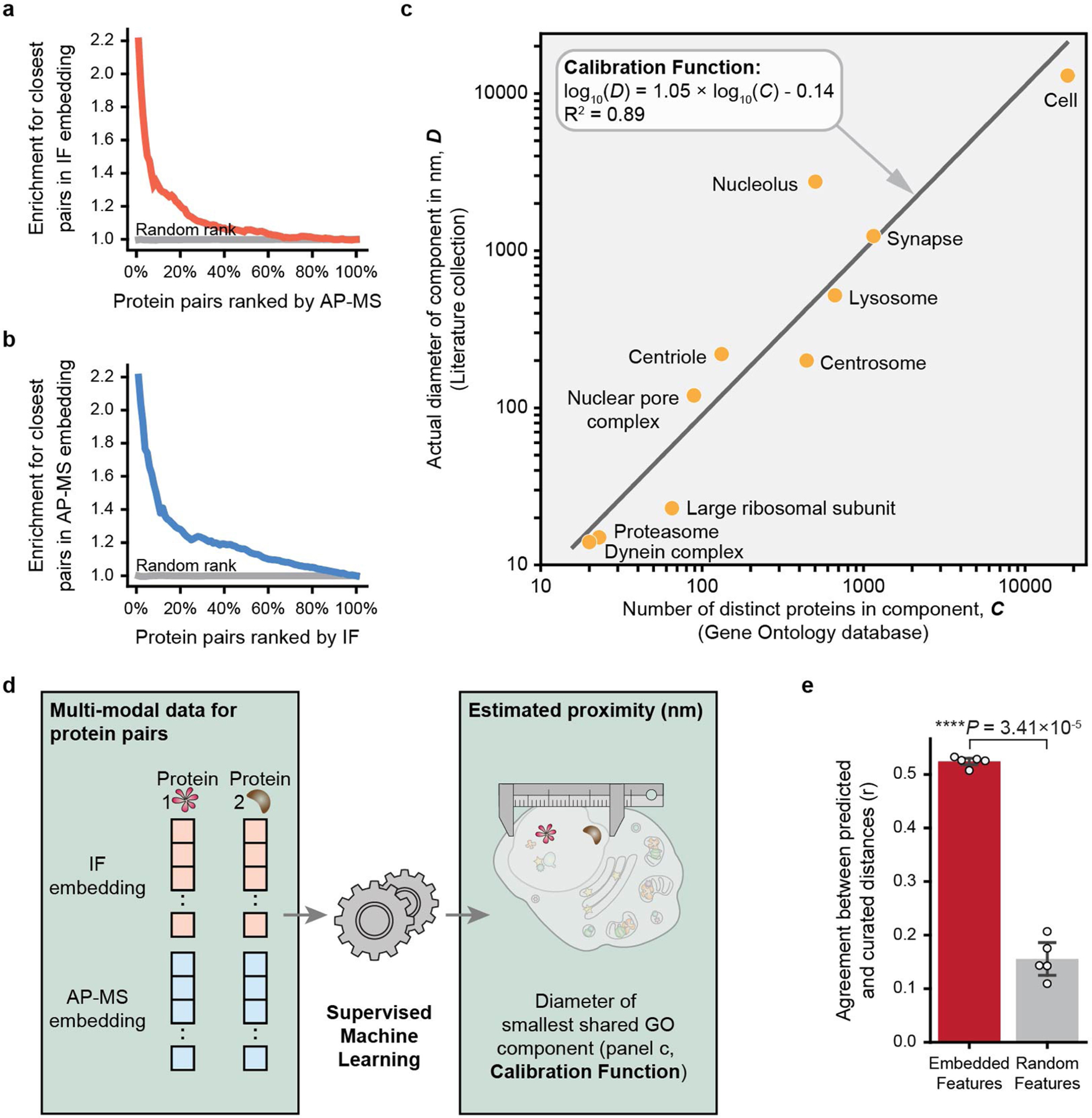
a, b, Protein pairs ranked by similarity in AP–MS embedding enrich for the most similar protein pairs in IF (a), and vice versa (b). c, Calibrating physical diameter, D, of subcellular components against the number of proteins, C, assigned to the corresponding Gene Ontology (GO) terms. d, Supervised model (random forest) estimates physical proximity (nm) of all pairs of proteins from their IF and AP–MS embeddings. e, Performance of model in recovering protein-protein distances in GO in five-fold cross validation (red, Pearson’s r). Equivalent calculation for random feature sets (grey). Statistics calculated using two-sided paired t-test. Data are presented as mean values +/− standard deviation.

Extended Data Fig. 4 |. Selection of parameters for community detection.

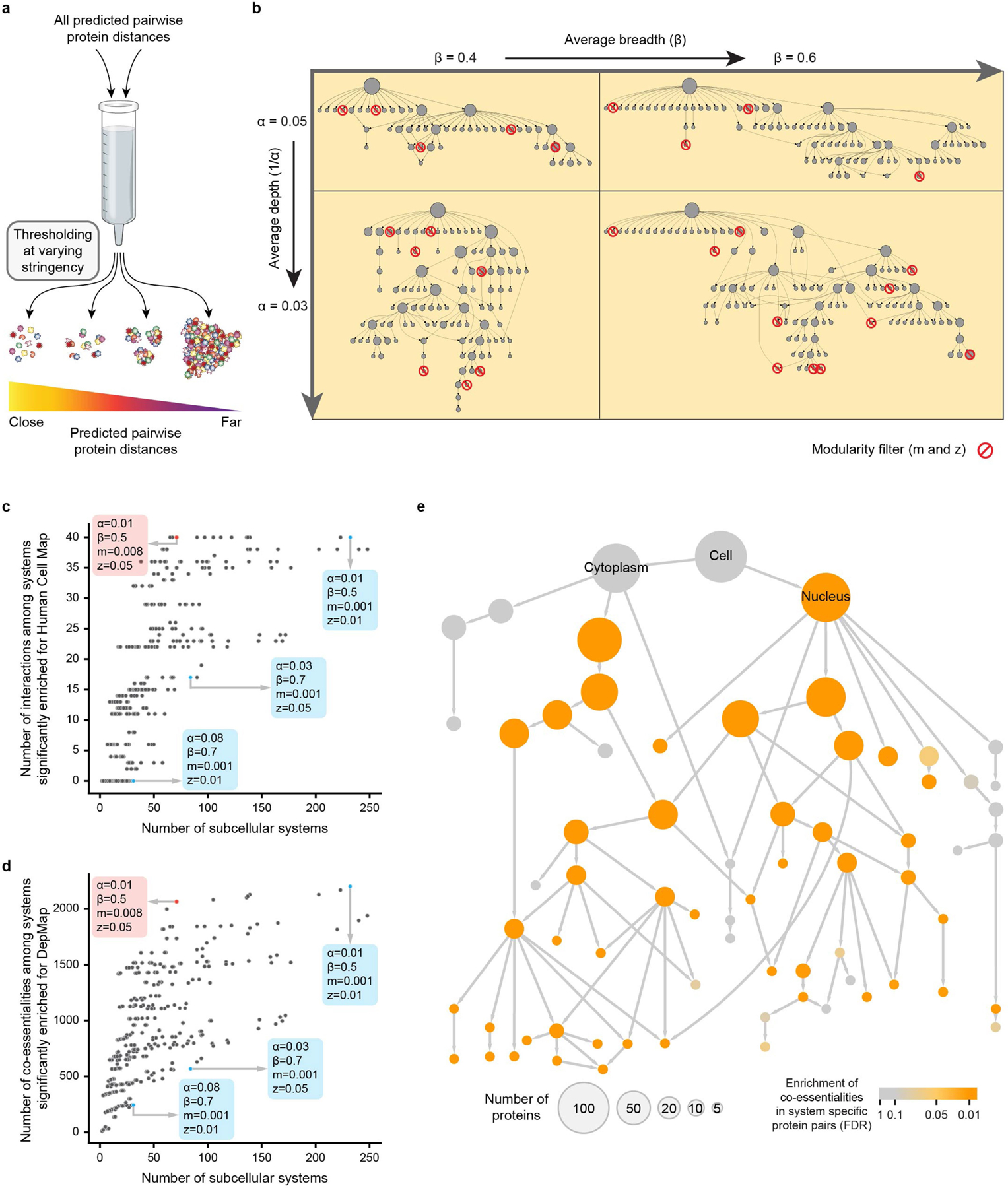
a, Using multi-scale community detection, protein systems of increasing sizes are discovered as the threshold for protein-protein distance is progressively increased. b, CliXO community detection has four parameters (depth α, y-axis; breadth β, x-axis; minimum modularity m and modularity significance z, red circle backslash) that affect the sensitivity with which communities are identified and thus the size of the hierarchy. c, d, Dot plots in which each dot is a community hierarchy generated with a particular set of parameters. The selection for MuSIC is highlighted in red. This selection was among several that were optimal based on enrichment for protein-protein interactions in Human Cell Map (c) and co-essentialities from DepMap (d). Examples of other parameter sets are shown in blue. e, Map from Fig. 2 with system colour showing enrichment for co-essentialities among protein pairs that are specific to that system. Enrichment of each system is assessed empirically, using 1,000 randomized hierarchies, followed by Benjamini–Hochberg multiple test correction to obtain FDR (orange gradient).

Extended Data Fig. 5 |. Supporting analyses for PRRPA.

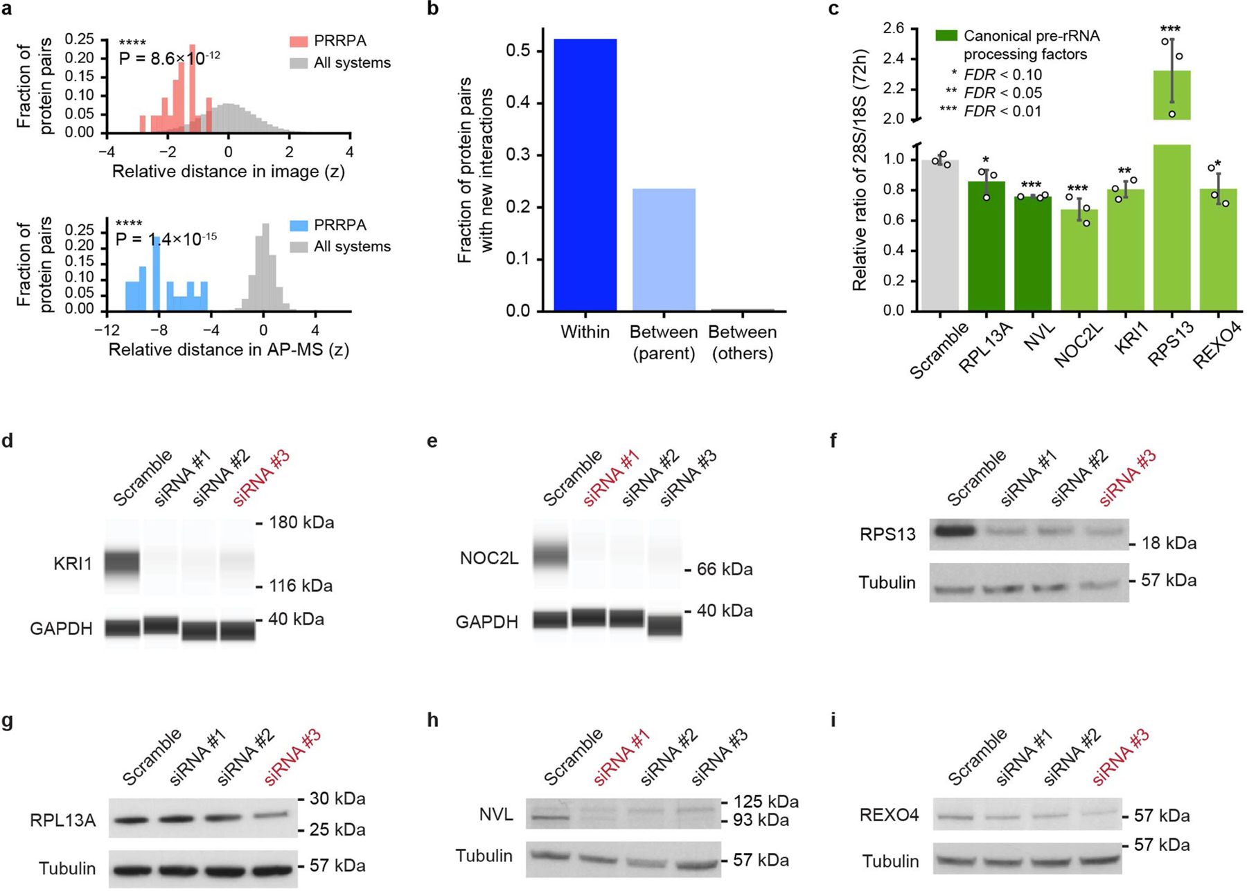
a, Distributions of protein-protein distance z-scores among the seven proteins in the PRRPA system for IF (top, red) or AP–MS (bottom, blue) modalities, calibrated to all such distances, respectively (grey). Statistics calculated using one-sided Mann–Whitney U test. b, Specific recovery of new AP–MS interactions within PRRPA is shown (dark blue bar), in comparison to interactions between proteins in PRRPA and other proteins organized under the same parent systems (“Ribosome” and “Ribosome biogenesis assembly”, light blue bar), or between proteins in PRRPA and those organized elsewhere in MuSIC (grey bar). c, Mature 28S/18S rRNA ratio under siRNAs targeting each PRRPA protein (green) versus scrambled siRNA (grey), n = 3 biological replicates. FDR from two-sided t-test with Benjamini–Hochberg correction. Data are presented as mean values +/− standard deviation. d–i, Western blot analysis (d, e, Simple western assay; f–i, SDS–PAGE) of target protein abundance after treating HEK293T cells with respective siRNA for 72 h (Supplementary Tables 6, 7). The siRNAs highlighted in red were selected to assess the perturbation of mature rRNA ratio (28S/18S rRNA) when knocking down target protein, with protein knockdown efficiency confirmed using western blot in three additional biological replicates. For source data, see Supplementary Fig. 1 (gel; d–i) and Supplementary Fig. 2 (total RNA profiles; c).

Extended Data Fig. 6 |. Supporting analyses for ribosomal systems.

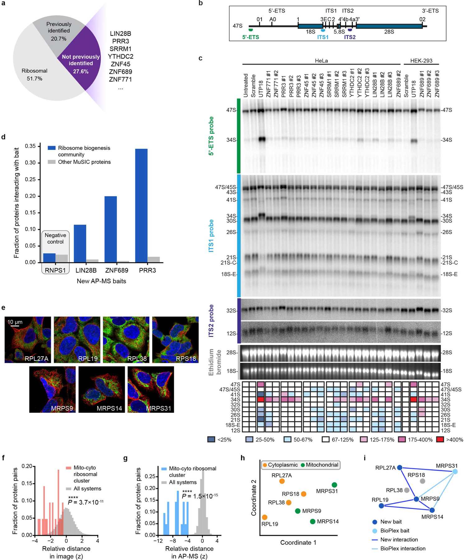
a, Categorization of proteins in “Ribosome biogenesis community” by whether they have been previously identified in human ribosome biogenesis. Excludes PRRPA proteins described in Fig. 5b–d. b, Structure of human pre-rRNA and probes used for northern blot. In eukaryotes, 3 out of 4 mature rRNAs (18S, 5.8S, and 28S rRNAs) are produced from a single long polycistronic precursor (47S) synthesized by RNA polymerase I. The mature rRNAs are interspersed with the 5′ and 3′ external transcribed spacers (ETS) and internal transcribed spacer (ITS) 1 and 2. The probes used in the northern blot (5′-ETS, ITS1, and ITS2) are indicated and colour-coded. c, Total RNA extracted from the indicated cell line, which was transfected with a DsiRNA specific to the target protein for 72 h and analysed by northern blotting with probes specific to the 5′-ETS, ITS1, and ITS2 sequences (Supplementary Table 8). As controls, cells were either untreated, transfected with a scrambled silencer, or transfected with a silencer targeting UTP18 (positive control involved in small ribosomal subunit biogenesis). Heat map colour shows the percentage of each pre-rRNA species with respect to the scramble control. For gel source data, see Supplementary Fig. 1. d, For protein baits in new AP–MS experiments (x axis), fraction of interacting preys that fall within the Ribosome biogenesis community (blue bars) versus elsewhere (grey bars). Only new AP–MS interactions are considered for this analysis. RNPS1 does not belong to Ribosome biogenesis community and serves as a negative control. e, IF images showing similar cytoplasmic staining for proteins in “Mito-cyto ribosomal cluster.” Cytoplasmic staining is dim for MRPS9, MRPS14 and MRPS31 compared to their predominant mitochondrial locations. Colours represent immunostained protein (green), cytoskeleton (red) and nucleus (blue). f, g, Corresponding distributions of protein-protein distance z-scores for IF (f, red) or AP–MS (g, blue), calibrated to all such distances, respectively (grey). Statistics calculated using one-sided Mann–Whitney U test. h, Two-dimensional projection of proteins in Mito-cyto ribosomal cluster, as in Fig. 5f. Proteins coloured according to known affiliations to cytoplasmic ribosome or mitochondrial ribosome. i, Validated AP–MS interactions in Mito-cyto ribosomal cluster. Note that only one out of seven proteins was previously tagged as bait in BioPlex 2.0 (light blue node), thus most physical associations (dark blue edges) among protein pairs were newly identified in this study.

Extended Data Fig. 7 |. Supporting analyses for chromatin regulation and splicing systems.

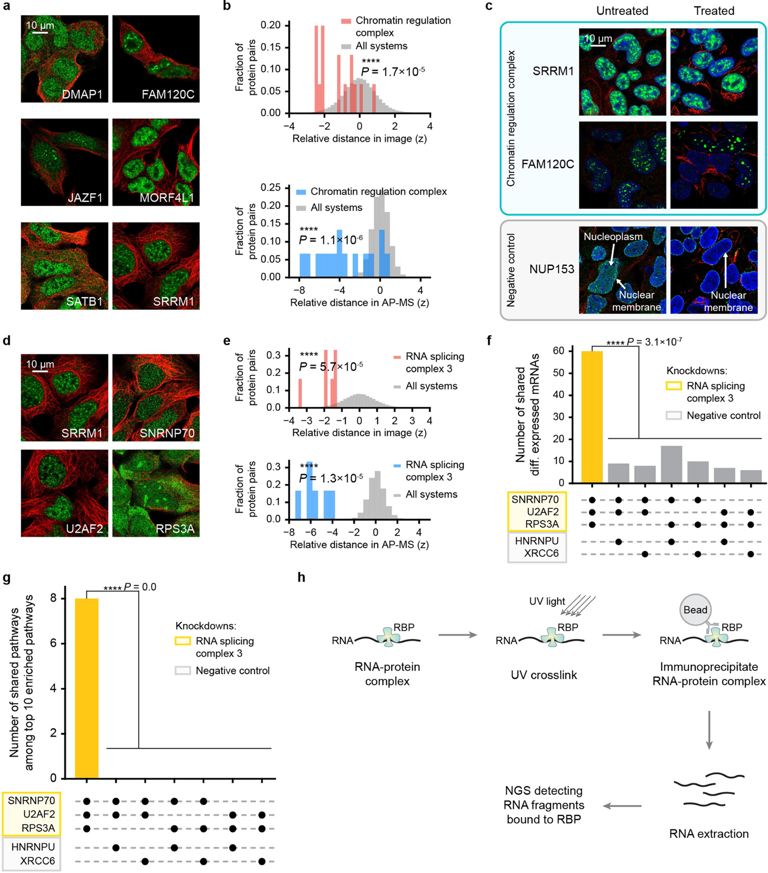
a, IF images showing similar nucleoplasm and nuclear speckles signals among proteins in the “Chromatin regulation complex.” Colours represent immunostained protein (green) and cytoskeleton (red). b, Distributions of pairwise protein distance z-scores among the proteins in the Chromatin regulation complex for IF (top, red) or AP–MS (bottom, blue) modalities, calibrated to all such distances, respectively (grey). Statistics calculated using one-sided Mann–Whitney U test. c, Immunofluorescent proteins (rows) imaged in HEK293 cells, untreated (left) or treated (right) with in situ fractionation to remove soluble cytoplasmic and loosely held nuclear proteins. Chromatin-binding proteins remain after treatment. Blue, nucleus; other colours as in a. For image source data, see Supplementary Fig. 3. d, IF images showing similar nucleoplasm signals among proteins in “RNA splicing complex 3.” e, Similar display for RNA splicing complex 3 as in b. f, Comparison of 500 top differentially expressed mRNAs (absolute fold change) resulting from shRNA knockdown of each of five genes (see Supplementary Table 9 for file accessions). Bar chart shows number of differential mRNAs shared by different gene groups indicated by black dots beneath each bar. One-sided one-sample t-test. g, Comparison among the top 10 pathways (Gene Ontology Biological Process) returned from Gene Set Enrichment Analysis using the top 500 differentially expressed transcripts. Bar chart shows number of enriched pathways shared by different gene groups indicated by black dots beneath each bar. One-sided one-sample t-test. h, eCLIP workflow. RBP, RNA-binding protein. NGS, next generation sequencing.

Extended Data Fig. 8 |. Supporting analyses for Discussion.

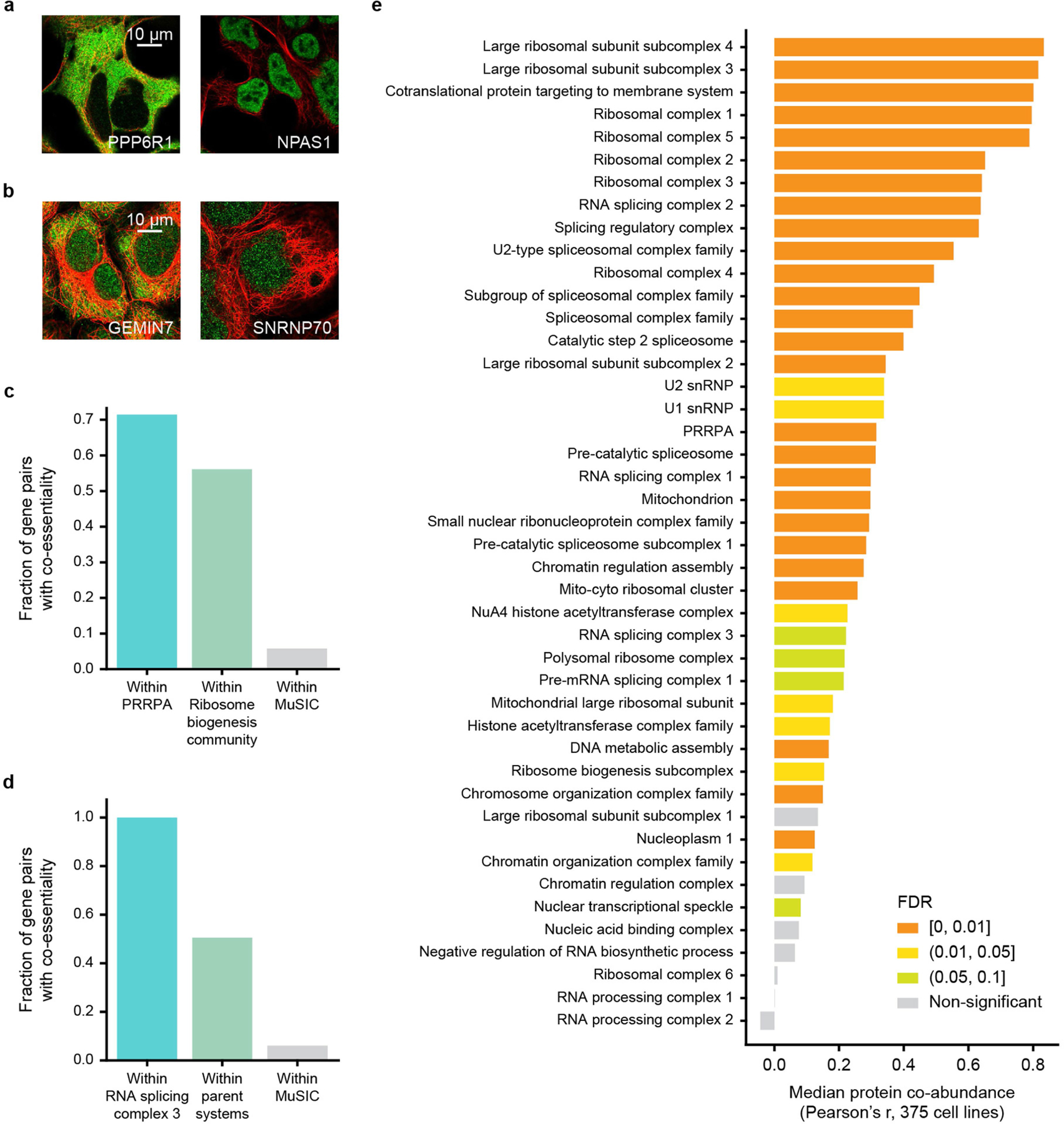
a, b, Examples of proteins with strong AP–MS protein interactions that have very different IF localization patterns. Colours represent immunostained protein (green) and cytoskeleton (red). c, Degree of co-essentiality for gene pairs within PRRPA (teal bar) shown in comparison to remaining pairs of genes assigned to the more general system that contains it, “Ribosome biogenesis community” (green bar), as well as all other gene pairs in MuSIC (grey bar). d, Similar analysis as in (c) for “RNA splicing complex 3.” Parent systems are “RNA processing complex 1” and “RNA splicing complex family.” e, Protein co-abundance for MuSIC systems, calculated from the median Pearson correlation of pairwise protein abundance over 375 diverse cell lines³². The plot shows all systems with fewer than 20 proteins and co-abundance measurements for >50% of protein pairs. Significance is assessed empirically (one-sided), using 1,000 randomized MuSIC hierarchies, followed by Benjamini–Hochberg multiple test correction to obtain FDR (colour of bar). Protein co-abundance for a system provides evidence for its presence in cell types beyond HEK293.

Data availability

A web portal is available at http://nrnb.org/music with links to all major resources used for this study. These include the MuSIC map (https://doi.org/10.18119/N9188W); the immunofluorescence (HPA) and AP–MS data (BioPlex 2.0) on which the map is based; and data for the AP–MS pull-down experiments performed as follow-up. The new AP–MS data have also been included as part of the larger compendium of protein interactions in the next version of the BioPlex resource (BioPlex 3.0²⁹). AP–MS data, including filtered and unfiltered interaction lists as well as raw mass spectrometry data, are also available at http://bioplex.hms.harvard.edu. The image data and associated metadata can also be found in the HPA database (https://www.proteinatlas.org). The Gene Expression Omnibus (GEO) accession number for eCLIP data generated in this study is GSE171553. Source data are provided with this paper.

References

- 1.Harold FM Molecules into cells: specifying spatial architecture. Microbiol. Mol. Biol. Rev 69, 544–564 (2005). [DOI] [PMC free article] [PubMed] [Google Scholar]
- 2.Mori H & Cardiff RD Methods of immunohistochemistry and immunofluorescence: converting invisible to visible. In The Tumor Microenvironment, Methods in Molecular Biology Vol. 1458 (eds Ursini-Siegel J & Beauchemin N) 1–12 (Humana Press, 2016). [DOI] [PubMed] [Google Scholar]
- 3.Aebersold R & Mann M Mass-spectrometric exploration of proteome structure and function. Nature 537, 347–355 (2016). [DOI] [PubMed] [Google Scholar]
- 4.Thul PJ et al. A subcellular map of the human proteome. Science 356, eaal3321 (2017). [DOI] [PubMed] [Google Scholar]
- 5.Huttlin EL et al. Architecture of the human interactome defines protein communities and disease networks. Nature 545, 505–509 (2017). [DOI] [PMC free article] [PubMed] [Google Scholar]
- 6.Schaffer LV & Ideker T Mapping the multiscale structure of biological systems. Cell Syst 12, 622–635 (2021). [DOI] [PMC free article] [PubMed] [Google Scholar]
- 7.Ouyang W et al. Analysis of the Human Protein Atlas Image Classification competition. Nat. Methods 16, 1254–1261 (2019). [DOI] [PMC free article] [PubMed] [Google Scholar]
- 8.Grover A & Leskovec J node2vec: scalable feature learning for networks. In KDD ‘16: Proc. 22nd ACM SIGKDD International Conference on Knowledge Discovery and Data Mining 855–864 (2016). [DOI] [PMC free article] [PubMed] [Google Scholar]
- 9.Goodfellow I, Bengio Y, Courville A & Bengio Y Deep Learning Vol. 1 (MIT Press, 2016). [Google Scholar]
- 10.Fortunato S & Hric D Community detection in networks: a user guide. Phys. Rep 659, 1–44 (2016). [Google Scholar]
- 11.Go CD et al. A proximity-dependent biotinylation map of a human cell. Nature 595, 120–124 (2021) [DOI] [PubMed] [Google Scholar]
- 12.Meyers RM et al. Computational correction of copy number effect improves specificity of CRISPR–Cas9 essentiality screens in cancer cells. Nat. Genet 49, 1779–1784 (2017). [DOI] [PMC free article] [PubMed] [Google Scholar]
- 13.Deckert J et al. Protein composition and electron microscopy structure of affinity-purified human spliceosomal B complexes isolated under physiological conditions. Mol. Cell. Biol 26, 5528–5543 (2006). [DOI] [PMC free article] [PubMed] [Google Scholar]
- 14.Charenton C, Wilkinson ME & Nagai K Mechanism of 5′ splice site transfer for human spliceosome activation. Science 364, 362–367 (2019). [DOI] [PMC free article] [PubMed] [Google Scholar]
- 15.Yoshikatsu Y et al. NVL2, a nucleolar AAA-ATPase, is associated with the nuclear exosome and is involved in pre-rRNA processing. Biochem. Biophys. Res. Commun 464, 780–786 (2015). [DOI] [PubMed] [Google Scholar]
- 16.Chaudhuri S et al. Human ribosomal protein L13a is dispensable for canonical ribosome function but indispensable for efficient rRNA methylation. RNA 13, 2224–2237 (2007). [DOI] [PMC free article] [PubMed] [Google Scholar]
- 17.Tafforeau L et al. The complexity of human ribosome biogenesis revealed by systematic nucleolar screening of pre-rRNA processing factors. Mol. Cell 51, 539–551 (2013). [DOI] [PubMed] [Google Scholar]
- 18.Eppens NA et al. Deletions in the S1 domain of Rrp5p cause processing at a novel site in ITS1 of yeast pre-rRNA that depends on Rex4p. Nucleic Acids Res 30, 4222–4231 (2002). [DOI] [PMC free article] [PubMed] [Google Scholar]
- 19.De Silva D, Tu Y-T, Amunts A, Fontanesi F & Barrientos A Mitochondrial ribosome assembly in health and disease. Cell Cycle 14, 2226–2250 (2015). [DOI] [PMC free article] [PubMed] [Google Scholar]
- 20.Blencowe BJ et al. The SRm160/300 splicing coactivator subunits. RNA 6, 111–120 (2000). [DOI] [PMC free article] [PubMed] [Google Scholar]
- 21.The UniProt Consortium. UniProt: a worldwide hub of protein knowledge. Nucleic Acids Res 47, D506–D515 (2019). [DOI] [PMC free article] [PubMed] [Google Scholar]
- 22.Pavan Kumar P et al. Phosphorylation of SATB1, a global gene regulator, acts as a molecular switch regulating its transcriptional activity in vivo. Mol. Cell 22, 231–243 (2006). [DOI] [PubMed] [Google Scholar]
- 23.Pomeranz Krummel DA, Oubridge C, Leung AKW, Li J & Nagai K Crystal structure of human spliceosomal U1 snRNP at 5.5 A resolution. Nature 458, 475–480 (2009). [DOI] [PMC free article] [PubMed] [Google Scholar]
- 24.Fleckner J, Zhang M, Valcárcel J & Green MR U2AF65 recruits a novel human DEAD box protein required for the U2 snRNP-branchpoint interaction. Genes Dev 11, 1864–1872 (1997). [DOI] [PubMed] [Google Scholar]
- 25.Van Nostrand EL et al. A large-scale binding and functional map of human RNA-binding proteins. Nature 583, 711–719 (2020). [DOI] [PMC free article] [PubMed] [Google Scholar]
- 26.Van Nostrand EL et al. Robust, cost-effective profiling of RNA binding protein targets with single-end enhanced crosslinking and immunoprecipitation (seCLIP). In mRNA Processing, Methods in Molecular Biology Vol. 1648 (ed. Shi Y) 177–200 (Humana Press, 2017). [DOI] [PMC free article] [PubMed] [Google Scholar]
- 27.Stryer L Fluorescence energy transfer as a spectroscopic ruler. Annu. Rev. Biochem 47, 819–846 (1978). [DOI] [PubMed] [Google Scholar]
- 28.Wang T et al. Gene essentiality profiling reveals gene networks and synthetic lethal interactions with oncogenic Ras. Cell 168, 890–903 (2017). [DOI] [PMC free article] [PubMed] [Google Scholar]
- 29.Huttlin EL et al. Dual proteome-scale networks reveal cell-specific remodeling of the human interactome. Cell 184, 3022–3040 (2021). [DOI] [PMC free article] [PubMed] [Google Scholar]
- 30.Williams SG & Hall KB Human U2B″ protein binding to snRNA stemloops. Biophys. Chem 159, 82–89 (2011). [DOI] [PMC free article] [PubMed] [Google Scholar]
- 31.Huang G, Liu Z, van der Maaten L & Weinberger KQ Densely connected convolutional networks Preprint at https://arxiv.org/abs/1608.06993 (2016).
- 32.Nusinow DP et al. Quantitative proteomics of the Cancer Cell Line Encyclopedia. Cell 180, 387–402 (2020). [DOI] [PMC free article] [PubMed] [Google Scholar]
Associated Data
This section collects any data citations, data availability statements, or supplementary materials included in this article.
Supplementary Materials
Data Availability Statement