Learning white matter subject-specific segmentation from structural MRI

Abstract

Purpose:

Mapping brain white matter (WM) is essential for building an understanding of brain anatomy and function. Tractography-based methods derived from diffusion-weighted MRI (dMRI) are the principal tools for investigating WM. These procedures rely on time-consuming dMRI acquisitions that may not always be available, especially for legacy or time-constrained studies. To address this problem, we aim to generate WM tracts from structural magnetic resonance imaging (MRI) image by deep learning.

Methods:

Following recently proposed innovations in structural anatomical segmentation, we evaluate the feasibility of training multiply spatial localized convolution neural networks to learn context from fixed spatial patches from structural MRI on standard template. We focus on six widely used dMRI tractography algorithms (TractSeg, RecoBundles, XTRACT, Tracula, automated fiber quantification (AFQ), and AFQclipped) and train 125 U-Net models to learn these techniques from 3870 T1-weighted images from the Baltimore Longitudinal Study of Aging, the Human Connectome Project S1200 release, and scans acquired at Vanderbilt University.

Results:

The proposed framework identifies fiber bundles with high agreement against tractography-based pathways with a median Dice coefficient from 0.62 to 0.87 on a test cohort, achieving improved subject-specific accuracy when compared to population atlas-based methods. We demonstrate the generalizability of the proposed framework on three externally available datasets.

Conclusions:

We show that patch-wise convolutional neural network can achieve robust bundle segmentation from T1w. We envision the use of this framework for visualizing the expected course of WM pathways when dMRI is not available.

1 |. INTRODUCTION

Mapping WM is essential to understand anatomy¹ and function.² DMRI works as the noninvasive imaging method to examine the white matter (WM) pathway in vivo. DMRI measures random microscopic motion (or diffusion) of water molecules in the brain tissue as the contrast parameter.³ The motion is anisotropic because of arrangement of fibers within WM. Based on this property, tractography is performed to estimate anatomical trajectories of WM. One popular workflow is to estimate local fiber orientation based on diffusion signal model like tensor⁴ or other advanced models^5,6 and reference long-range pathways from local orientation.⁷ The subsequent dissection⁸ of streamlines across from whole-brain tractograms allows for the segmentation or mapping of WM pathways.

In order for DMRI to be appropriate for tractography, many gradient directions and high b-value shells are needed, which are not commonly acquired in clinical settings and require long scan times.⁹ The computation and dissection of whole brain tractograms derived from tractography is also time-consuming, which limits the applicability of tractography in time-constrained settings. Structural T1 weighted (T1w) MRI acquisitions are widely used in neuroimaging research and in the clinical setting. However, it is challenging to directly delineate WM pathways from T1w MRI, as the lack of directionality information of bundles in T1w.

Fortunately, image registration is an established way of transferring different WM labels from population-based atlases to T1w MRI and can isolate different WM regions in T1w MRI. In general, WM atlases from the diffusion-weighted MRI (dMRI) community can be divided into two categories: streamline-based atlases^10–13 and volumetric atlases.^14–16 Streamline-based WM atlases contain streamlines assigned to various WM pathways, while volumetric WM atlases contain labels indicating the pathway assignment(s) of a given voxel. One such widely used volumetric atlas was proposed by Mori et al. and recognizes 48 different WM labels.¹⁵ WM atlases are very popular in neuroimaging analysis but have key limitations. They require that different WM regions are not overlapping and often contain a limited amount of information outside deep WM (Figure 1). To navigate these limitations, Hansen et al. recently proposed the Pandora WM bundle atlases, which are volumetric atlases that present 216 overlapping WM pathways from 2300 healthy subjects. This approach has subsequently allowed for both the identification of overlapping pathways and improved WM labeling outside the deep structures on T1w MRI without dMRI.¹⁶

FIGURE 1.

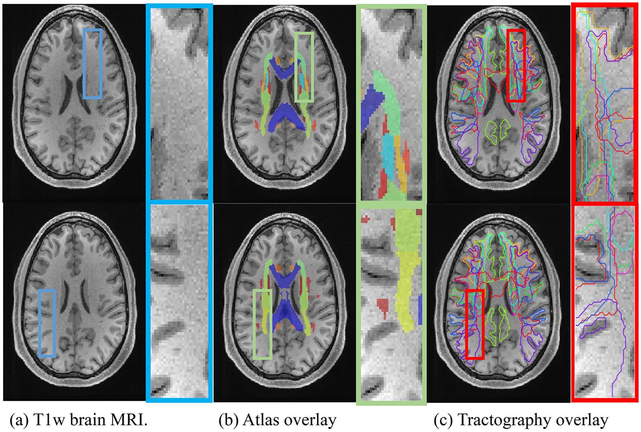
(a) White matter (WM) is largely homogenous when imaged using most sources of MRI contrast, for example T1 weighted (T1w) (left).(b) Traditional WM atlas (center) represents each voxel with one tissue class. (c) Modern approaches at bundle segmentation identify multiple overlapping structures (right). Diffusion tractography offers the ability to capture a multi-label description of WM voxels

Compared with large cohort population atlas, deep convolutional neural networks have the potential to capture subject-specific variations. Among convolutional neural networks, the U-Net¹⁷ has obtained impressive results for performing 3D medical image segmentation including brain¹⁸ and abdomen.¹⁹ Brébisson et al. proposed a deep neural network learning 2D and 3D patches from structural brain MRI to predict the anatomical class of each voxel.²⁰ DeepNat leverages a hierarchical multi-task network to achieve brain segmentation with 3D patches.²¹ SLANT¹⁸ learns spatially localized 3D patches from structural MRI to achieve brain structure segmentation. Additionally, current deep learning approaches^20,22 have demonstrated superior performance compared with atlas-based methods on healthy brain segmentation from structural images.

Thus, driven by the need for improved subject-specificity in WM segmentation, we propose a spatially localized patch-wise framework to delineate WM regions from structural T1w MRI. We envision this framework as a tool for researchers to localize WM regions when dMRI is not available. To make this tool comprehensive, we select six state-of-the-art tractography algorithms.

2 |. MATERIAL AND METHODS

The pipeline of predicting WM labels directly from T1w MRI with deep learning includes four steps:tractography, registration, normalization, and patch-wise networks as shown in Figure 2.

FIGURE 2.

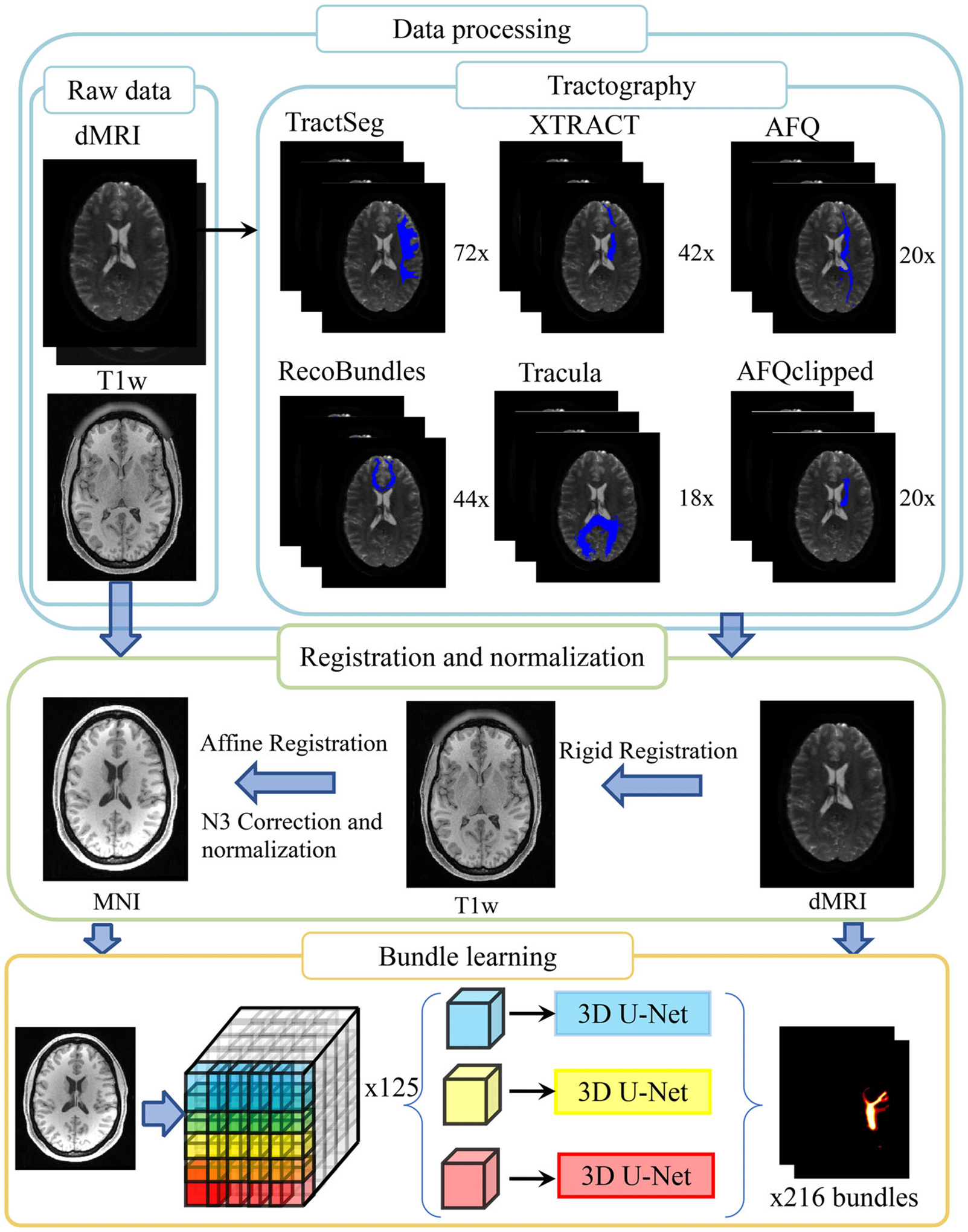
The pipeline of proposed white matter (WM) bundle learning is presented, which integrates data processing and registration as well as bundle learning. We extract WM bundles from six different tractography methods. Structural images and corresponding tractograms are reoriented to the Montreal Neurological Institute (MNI) template. Patch-wise, spatial-localized neural networks are utilized to learn WM bundle regions from a T1 weighted (T1w) MRI image. The output of each U-net is merged as the final step before segmentation. Representative samples of WM bundles acquired from six automatic tractography methods, and the final learning result is visualized

2.1 |. Data

We use 2416 deidentified images from the Baltimore Longitudinal Study of Aging (BLSA),²³ 1105 images from Human Connectome Project S1200 release,²⁴ and 349 images from Vanderbilt University (VU) to train all deep neural networks. We also select three open-source datasets to perform external validation to test the generalizability of the proposed learning method. We study 26 images from HCP lifeSpan (HCPLS),²⁴ 394 images from IXI (IXI, http://brain-development.org/ixi-dataset), and 12 images from the Unilateral Glaucoma dataset (UG, https://openneuro.org/datasets/ds001743/versions/1.0.1). All above images include paired T1w MRI and dMRI. The voxel resolution of T1w MRI and dMRI, the b0-value and diffusion volumes are shown in Table 1.

TABLE 1.

Dataset descriptions

Dataset name	T1w voxel size (mm)	Diffusion voxel size (mm)	B-value	Diffusion volume
BLSA	1.0 ×1.0 × 1.2	0.81 × 0.81 × 2.2	700	1B0 + 32DWIs
HCP	0.7 × 0.7 × 0.7	1.25 × 1.25 × 1.25	1000,2000,3000	(6B0 + 90DWIs) ×3
VU*	1 × 1× 1	2.5 × 2.5 × 2.5	1000	1B0 + 64DWIs
HCP_LS	0.8 × 0.8 × 0.8	1.5 × 1.5 × 1.5	1000,2500	5B0 +76DWIs
IXI	0.93 × 0.93 × 1.2	1.75 × 1.75 × 2.35	1000	1B0 + 15DWIs
UG	1 × 1 × 1	2 × 2 × 2	2000	6B0 + 48DWIs

Abbreviations: BLSA, Baltimore Longitudinal Study of Aging; HCP, Human Connectome Project; VU, Vanderbilt University.

^*Represents one typical case selected from the VU dataset.

2.2 |. Tractography

dMRI is often subject to artifacts, which can deteriorate the accuracy of extracting WM bundles. To correct these artifacts, we perform correction for susceptibility distortions, subject motion, eddy currents, and b-tables prior to analysis.²⁵

We perform tractography on preprocessed dMRI. Six popular tractography algorithms are selected to recognize pathways and annotate WM bundles. All six algorithms were run using default parameters. The number of generated pathways of all six tractography algorithms is shown in Table 2.

TABLE 2.

The tractography algorithms and corresponding generated pathways

The algorithm name	Number of generated bundles for each algorithm
TractSeg26	72
RecoBundles27	44
XTRACT28	42
Tracula29	18
AFQ30	20
AFQclipped30	20

Note that AFQclipped clips the center of each of the 20 AFQ bundles with region of interests (ROI)-based exclusion criteria. According to anatomic name for each bundle, we notice that there are 10 common bundles across from all six tractography algorithms. Thus, 216 bundles from TractSeg, RecoBundles, XTRACT, Tracula, AFQ, and AFQclipped are not regarded as unique bundles.

2.3 |. Registration and intensity normalization

To ensure that all inputs have the same voxel size and dimension, we register all pathways derived from dMRI through all six bundle segmentation algorithms and T1w MRI, to the Montreal Neurological Institute (MNI) ICBM 152 asymmetric template.³¹ First, we rigidly register the b = 0 s/mm² volume of each dMRI to the T1w MRI of the same subject using FMRIB’s software library (FSL).³² Then, after performing N3 correction of bias field and normalization of WM intensity by FreeSurfer³³ on raw T1w MRI, corrected T1w MRI is registered to the MNI template with antsRegistrationSyn in advanced normalization tools (ANTs).³⁴ By linking these registration steps, all pathways are rigidly registered to T1w MRI of the same subject. All pathways are affine reoriented to the MNI template and serve as ground truth. The affine transformation is also applied to the raw T1w MRI.

After registration, we skull strip all structural images on the MNI template with the bet tool in FSL, clip, and normalize the background and the 98th percentile of within-brain intensity to intensity units 0 and 1. The pipeline of registration and normalization is visualized in the Figure 2

2.4 |. Patch-wise network

After transforming all image and ground-truth pathways to MNI template, the high-resolution image volume could not fit into the 12G GPU (GTX 1080Ti) memory using current popular network architectures. Inspired by SLANT,¹⁸ we designed 125 overlapped 3D U-Nets to cover the entire MNI volume and subdivide each image into corresponding 125 patches. Each patch Ψ_n is represented by one coordinate (x_n, y_n, z_n) and patch size (d_x, d_y, d_z), n ∈ {1, 2, … 125}

$${\psi }_n=\left[x_n:\left(x_n+d_x\right),y_n:\left(y_n+d_y\right),z_n:\left(z_n+d_z\right)\right]$$ (1)

where Ψ_n represents the nth patch, x_n, y_n, z_n represent the corner coordinates of the nth patch. x_n and z_n ∈ [1, 25, 50, 74, 98] and y_n ∈ [1, 34, 67, 101, 134]. The length d_x, the width d_y, and depth d_z are 96.

To merge the outputs of the U-Nets after training, the pixel-wise output represents an activation value of the neural network rather than specific WM pathways. Thus, the average way is adopted to get the final value instead of majority vote:

$$p_{\text{whole}}(i)=\frac{1}{n_k}\sum _{k=1}^{n_k}{p}_k(i)$$ (2)

Where p_whole represents all pixels within the structural, image and p_whole(i) means the ith pixel. k indexes the U-Nets that covers ith pixel. p_k(i) represents the final value of ith pixel of kth U-net. Networks not covering a particular voxel are excluded in the final merge process.

2.5 |. Implementation details

We divided the HCP, BLSA, and VU data into training, validation, and test cohorts evenly based on subjects and used HCP_LS, IXI and unilateral glaucoma (UG) as the external dataset. We kept the splitting strategy consistent across learning all six diffusion tractography algorithms. To remove data corrupted by registration or failed diffusion tractography algorithms, exhaustive human review was performed on verifying acceptable image registration and inspecting appropriate shape and location of all bundles.¹⁶ The resultant number of scans for the training, validation, testing cohorts, and external dataset is shown in Table 3.

TABLE 3.

The number of scans for the training, validation, testing cohorts, and external dataset

	Scans of train	Scans of validation	Scans of test	Scans of external validation
TractSeg	2803	213	754	431
RecoBundles	2789	211	754	430
XTRACT	2786	211	751	427
Tracula	2538	189	693	428
AFQ	2730	201	726	367
AFQclipped	2730	201	726	367

Inspired by the AssemblyNet,³⁵ we adopt a transfer learning technology to utilize the weights from trained U-Net to initialize the nearest U-Nets. In the beginning, we trained nine U-Nets, and their corner coordinates are shown in Table 4. Then, the trained nine models following orders in the Table 4 are used to initialize the nearest 116 models (every model is trained only once).

TABLE 4.

Corner coordinates of pretrained nice models of 125 models, indexed starting at one

Corner coordinate index	Corner coordinate (x, y, z)
2, 2, 2	25, 34, 25
2, 4, 2	25, 101, 25
4, 2, 2	101, 25, 25
4, 4, 2	101, 101, 25
3, 3, 3	50, 67, 50
2, 2, 4	25, 34, 74
2, 4, 4	25, 101, 74
4, 2, 4	101, 25, 74
4, 4, 4	101, 101, 74

We used pytorch³⁶ to implement baseline U-Net¹⁷ as the convolution neural network to learn patches from anatomical images and set the batch size 1. The output channel depends on the number of WM bundles recognized by the bundle segmentation algorithm. We set a learning rate of 0.0001 and do not perform learning rate decay during the training process. We adopted the sum binary cross-entropy for each effective WM bundle as a loss function and train all models using the Adam optimizer. When we inferred the WM regions based on deep neural networks, we appended a sigmoid function to the output of each patch-wise neural network to map the final merged output to (0, 1).

2.6 |. Baseline methods

We compare the quantitative performance of transferring labels with the traditional atlas-based approach as the baseline method. Here, we use the Pandora atlas,¹⁶ which is a 4D collection population-based atlases. The Pandora atlas used the same cohorts and diffusion tractography algorithms to generate each corresponding WM bundle same as we learn in this study. All volumes of the Pandora atlas are on the same MNI template as we use here. Each volume of the 4D atlas is in the form of a probability map indicating a probability of a pixel being in a specific WM bundle. To make a fair comparison, we transfer label from atlas to affine-reoriented MNI template as final probability map for each target scan.

In addition to atlas-based method, we use multi-atlas segmentation (MAS) as another baseline method. We selected 20 subjects whose tracts all passed human review as single atlas. There are nine subjects from HCP, nine subjects from BLSA, and two subjects from VU among 20 subjects. To make sure output is in the same template as other comparison methods, all 20 atlas and target images are affine reoriented to MNI template as well as the corresponding WM tracts. All 20 atlases are registered to target image through non-rigid registration.³⁷ Then, the new labels are obtained through joint label fusion³⁸ methods. The whole pipeline of MAS is implemented by ANTs³⁹ python package and performed for all 216 bundles for each target scan.

2.7 |. Metrics

To evaluate the accuracy of our proposed method, we compare the segmentation results against the ground truth provided by diffusion tractography. Additionally, we compare the accuracy of the proposed method against the accuracy achieved by Pandora atlas and MAS. To quantify the agreement between segmentation and truth, we use four measures: Dice score coefficient (DSC), average symmetry surface distance, bundle overlap, and bundle overreach.

We use DSC as the main evaluation measurement for different bundle segmentation algorithms by comparing binary WM bundle prediction against the ground truth voxel-by-voxel:

$$\text{DSC}=\frac{2\left|R\cap T\right|}{\left|R\right|+\left|T\right|}=\frac{2\left|\text{TP}\right|}{2\left|\text{TP}|+|\text{FP}|+|\text{FN}\right|}$$ (3)

where TP is true FP false positive, FN is false negative, R represents the segmentation result generated by the proposed method or atlas-based method, and T represents the corresponding ground-truth.

Average symmetry surface distance⁴⁰ is given in millimeters and based on surface vertices between the proposed or atlas-based segmentation, R, and the ground-truth segmentation, T. For each vertex on the surface of R, (S(R)), the Euclidean distance to closest surface vertices of truth (S(T)) can be defined in d(S_R, S(T)):

$$d\left(S_R,S(T)\right)=\underset{S_R\in S(R)}{\text{min}}\parallel S_R-S(T)\parallel \text{ASSD}=\frac{1}{\left|S(R)\right|+\left|S(T)\right|}\times \left(\sum _{s_R\in S(R)}d\left(s_R,S(T)\right)+\sum _{s_T\in S(T)}d\left(s_T,S(R)\right)\right)$$ (4)

where |S(R)| represents the number of vertices of the resulting surface, and |S(T)| represents the number of vertices on the ground-truth surface. S_R represents a vertex from the atlas-based or proposed segmentation. S_T represents a vertex from the ground-truth.

Bundle overlap⁴¹ is the proportion of voxels that contain the ground truth region that is also overlapped by the results of the learning- or atlas-based methods.

$$\text{OL}=\frac{R\cap T}{T}$$ (5)

Bundle overreach⁴¹ is the number of voxels containing results from proposed or atlas-based methods that are outside of the ground truth volume divided by the total number of voxels within the ground truth.

$$\text{OR}=\frac{R\backslash T}{T}$$ (6)

where operator \ denotes the relative complement operation.

The nonparametric Wilcoxon signed-rank test⁴² for paired distributions was used to calculate test significance when comparing learning-based results with corresponding atlas-based results.

3 |. RESULTS

3.1 |. Fine-tune binary threshold

The outputs of the MAS, atlas-based and proposed methods have been mapped to (0, 1) and represent a probability that a given voxel is included in the WM pathway. The binary threshold to convert the probability to a yes or no is important and influences the performance of both the atlas-based and proposed methods. Starting from 0, we sweep thresholds until 1 with a step size of 0.01, using the validation datasets to calculate mean DSC across all WM pathways of all scans. The optimal threshold and the curve of relationships between mean DSC and binary threshold for the MAS, atlas-, and learning-based methods are shown in Figure 3. The optimal thresholds are the values where the mean DSCs across all pathways from all scans are highest for MAS, atlas- and learning-based methods.

FIGURE 3.

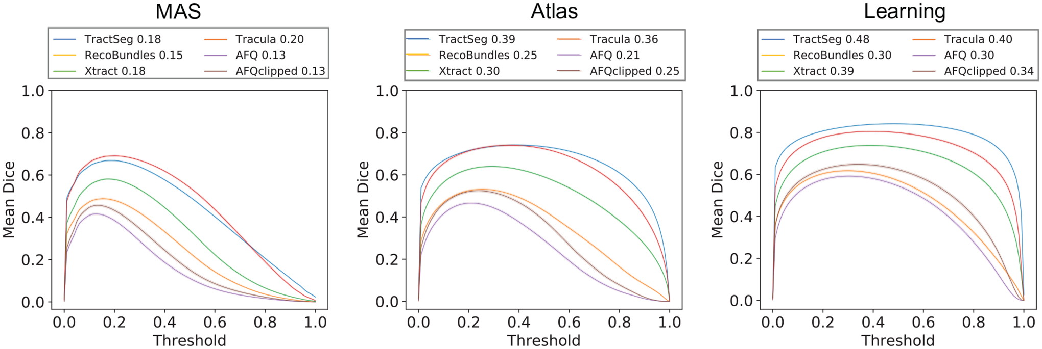
Each curve represents the average DSC of all white matter (WM) bundles of all validation dataset scans per diffusion tractography algorithms for multi-atlas segmentation (MAS), atlas-, and learning-based methods at different threshold values. The 95% confidence interval is within the printed notch due to large sample population size. The legend above the each plot includes the optimal threshold for each tractography algorithms

3.2 |. Qualitative results

We select one scan from the HCP test cohort to visualize the left corticospinal tract (CST) across all six bundle segmentation algorithms to see an intra-subject variance of bundle segmentation algorithms and visualize the difference between results derived from T1w images and ground truths from dMRI. We use the optimal threshold values calculated in Figure 3. to binarize each output, using marching cube⁴³ to extract and render the CST surface. 3D visualization is shown in Figure 4.

FIGURE 4.

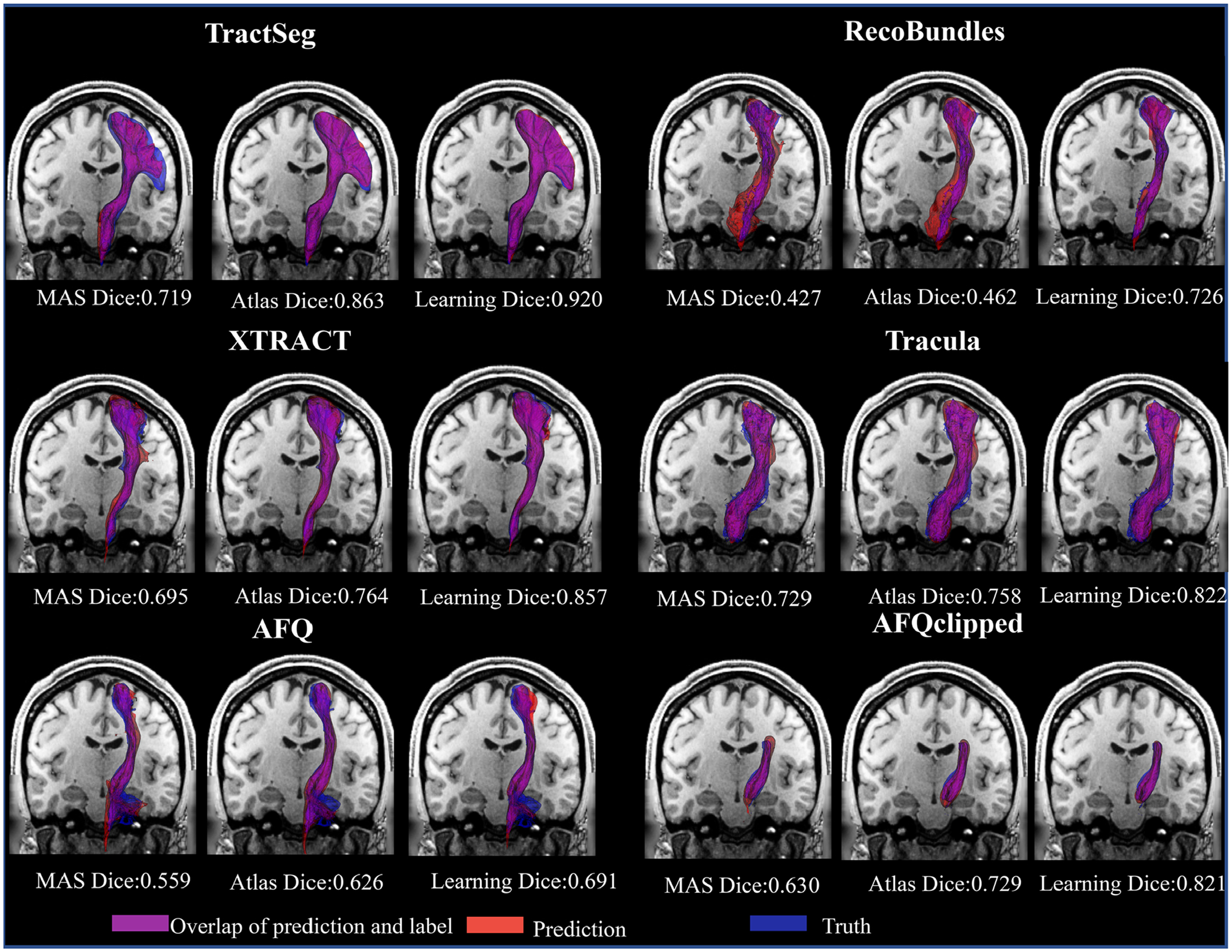
3D visualization of multi-atlas segmentation (MAS), atlas-, and learning-based results across six diffusion tractography algorithms by reconstruction of the left corticospinal tract (CST) surface on an affine-reoriented coronal T1 weighted (T1w) MRI slice. The text below each image is quantitative DSC for each case

From Figure 4, we find the learning-based method per bundle segmentation algorithm has a higher overlap compared with the atlas-based method and MAS according to the areas of magenta overlap for this subject. Although the pathway of all six tractography algorithms has varied shape, the learning method still can make good prediction for the largest pathway of TractSeg and smallest pathway of AFQclipped.

3.3 |. Quantitative results

We used the optimal threshold values fine-tuned from the validation datasets to binarize the output on the testing and external datasets. To examine their overall performance, we evaluated all 216 bundles using the DSC and average symmetry surface distance (Figure 5).

FIGURE 5.

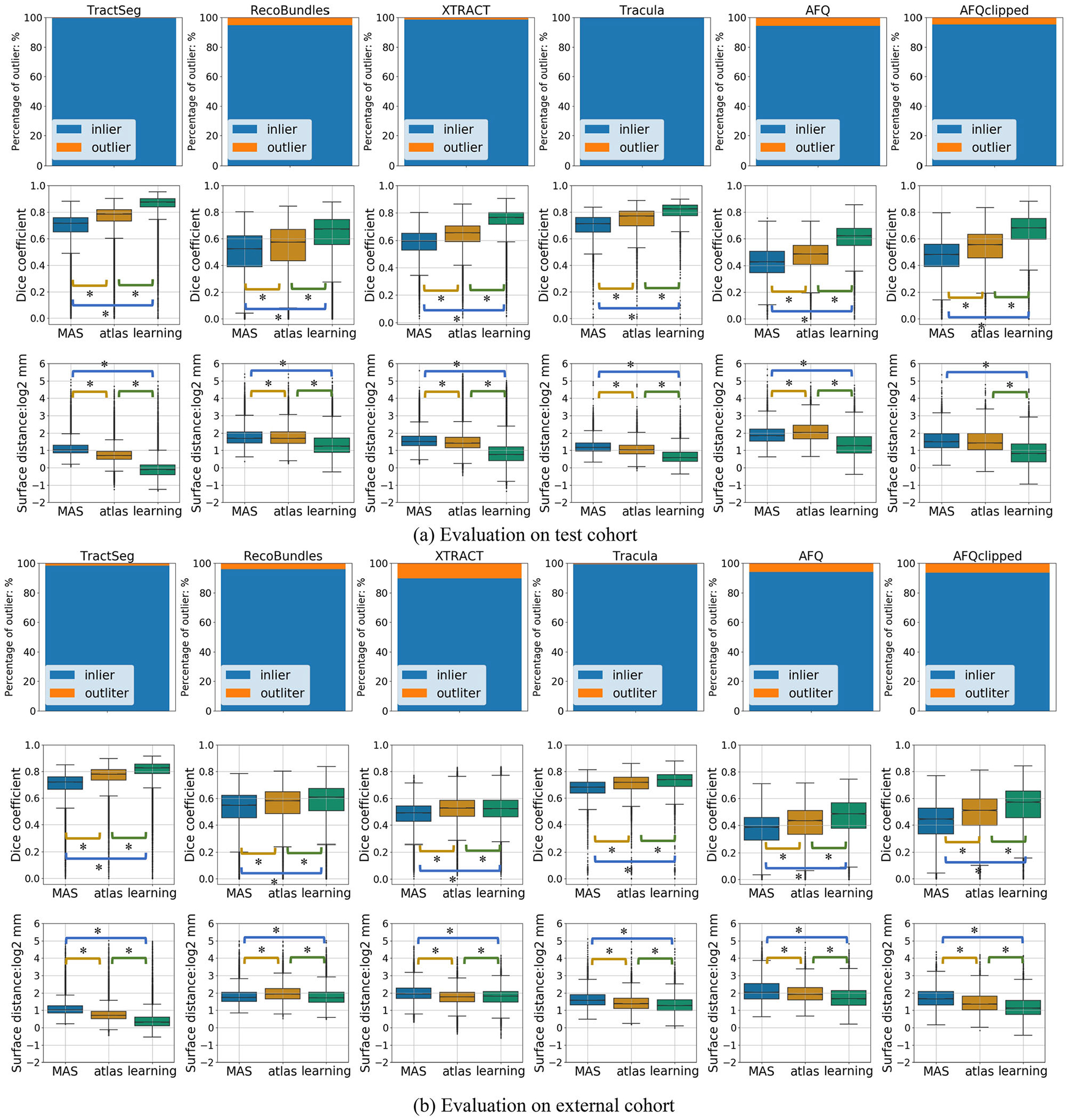
Quantitative results of multi-atlas segmentation (MAS), atlas-based method, and proposed learning methods on test cohorts from Human Connectome Project (HCP), Baltimore Longitudinal Study of Aging (BLSA), and Vanderbilt University (VU) and external cohort from HCP_LS, IXI, and UG. The outlier percentage (top row) of all six algorithms is shown in bar plot. Two measures are used to assess the overlap between algorithms deriving fiber mask from T1 weighted (T1w) and truth from diffusion-weighted MRI (dMRI): Dice (middle row) and surface distance (lower row). Each column presents the result of a different bundle segmentation algorithm and shows the proposed method, MAS, and single atlas-based method. Each boxplot includes each pathway of the bundle segmentation algorithm per every scan. The 95% confidence interval is within the printed notch due to large sample size. The difference between methods was significant (p < 0.005, Wilcoxon signed-rank test, indicated by *)

From Figure 5a, the blue bar plot represents the percentage of pathways that successfully passed the human reviewing process across the whole test cohort. All learning-based methods perform statistically better than the atlas-based methods and MAS. When using ground truths derived from TractSeg, the MAS, atlas- and learning-based methods achieve the highest median DSC of 0.72, 0.78, and 0.87 and smallest average symmetry surface distance 2.04 mm, 1.62 mm, and 0.92 mm, respectively. Compared with the atlas method, the learning method shows the largest improvement in median DSC for AFQ from 0.48 to 0.62 and reduces median average symmetry surface distance from 4.08 mm to 2.40 mm. The same pathway for different subjects may have varied shape and localization. The proposed method can adapt to these differences more robustly than atlas-based methods.

In Figure 5b, the blue bar plot represents the percentage of pathways that successfully passed the human reviewing process across the external dataset. All learning-based methods perform statistically better compared to atlas-based methods except for XTRACT. However, the difference between the atlas- and learning-based methods is less pronounced. The median DSC of the learning-based method on XTRACT is 0.522, lower than 0.527 of the atlas-based method. Compare Figure 5a,b, variations in MRI contrast across scanners decreases the performance.

We perform bundle overlap and bundle overreach on left CST pathway of all six bundle segmentation algorithms to analyze the relationship between spatial overlap of proposed method and threshold (Figure 6).

FIGURE 6.

Plots of overlap versus overreach for the left corticospinal tract (CST) across all bundle segmentation algorithms for multi-atlas segmentation (MAS), atlas-, and learning-based methods are shown. The markers on each curve to represent the overlap and overreach values at specific threshold values. The range of overreach for MAS is (0, 6). The range of overreach for atlas-based methods is (0, 9). The range of overreach for the learning-based method is (0, 6)

From Figure 6, all MAS, atlas- and learning-based methods for all six diffusion tractography algorithms identified WM bundles with a high overlap but suffer from high overreach except for Tracula and TractSeg. As for AFQ, when the overreach is about five times the actual ground truth volume, the MAS method has overlap values of 0.75 and 0.8 with the atlas-based method. The proposed method has an overlap value about 0.9 higher compared with the MAS and atlas-based method.

We calculated the overall binary thresholds from the validation cohort. Thus, we want to investigate whether the optimal thresholds calculated from validation datasets can generalize to external datasets. We show the curve of relationship between DSC and binary threshold on the external datasets in Figure 7. Comparing Figure 7 to Figure 3 the biggest difference between thresholds estimated from the validation dataset and the external datasets is in XTRACT. The binary threshold for MAS is shifted from 0.18 to 0.34. The binary threshold for atlas-based method in XTRACT is shifted from 0.30 to 0.56. The binary threshold for the proposed method in XTRACT is shifted from 0.39 to 0.77. We can learn that the optimal threshold shifts when fed different MRI contrast.

FIGURE 7.

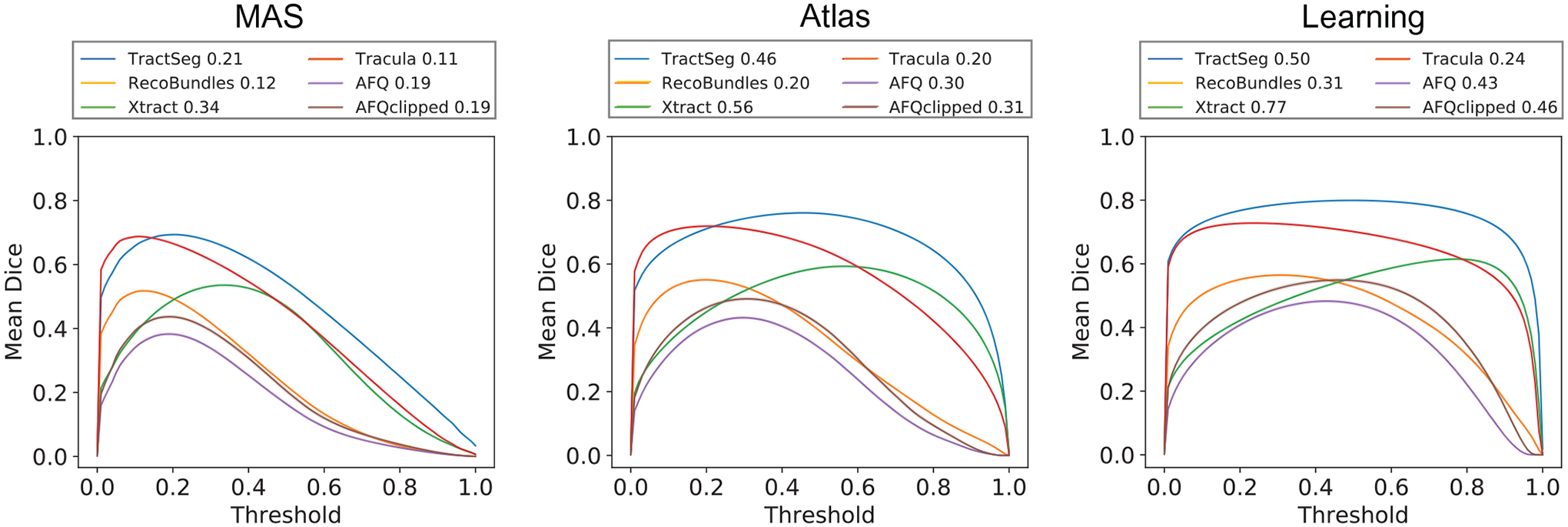
Each curve represents average DSC of all white matter (WM) bundles of all external dataset scans per diffusion tractography algorithm for atlas- and learning-based methods. The 95% confidence interval is within the printed line width due to large sample size. The legend above each plot includes the optimal threshold for each tractography algorithms

4 |. DISCUSSION

In this study, we aim to propose a spatial localized patch-wise framework to segment WM structure with six different definition schemes only from anatomical images. We envision this framework as a tool to estimate a coarse WM region of interest rather than segmentation with more details derived from dMRI. We provide probability map of six different tractography algorithms for users to adjust binary threshold and choose their preference scheme.

4.1 |. Generalize to external dataset

Deep learning model is sensitive to intensity distributions of T1w MRI, which are not seen in the training cohort. The different scale settings of the raw T1w images bring the shift of the optimal threshold, which is shown in the external dataset. Apart from varied intensity distribution, the external dataset itself also deteriorates the performance of deep neural network. 394 IXI images domain the whole dataset. The acquisition of IXI requires 15 DWIs, which is smaller compared to the original training cohort. Thus, generated ground truth by six algorithms does not have high quality (they might have less streamlines or streamlines stop in advance during the tracking process).

4.2 |. Limitations

Currently, the variance of performance of learning-based method is obvious. Inherent definition and way of extracting WM tracts by bundle segmentation methods bring challenges to the proposed learning framework. One possible solution is developing robust labels by merging common labels belonging to same WM bundle across from all six tractography algorithms. By doing this way, each WM bundle label will include six bundle definition schemes, having common parts and specific parts for each tractography algorithm. The robust label may make full use of complementary information among six tractography algorithms.

WM pathways usually are in the form of streamlines, which can provide connection at the sub-pixel level. However, information is lost when converting streamlines into mask, even with their own built-in function, which bring the noise to the label.

5 |. CONCLUSION

We propose a spatial localized patch-wise framework to delineate WM structure based on structural T1w images. We use this framework to learn WM regions under six bundle segmentation algorithms and compare the result of the framework to atlas-based methods and MAS. When optimal threshold is utilized to evaluate scans that have the same acquisition as the training datasets, the learning-based methods are statistically superior to the atlas-based methods and MAS.

All source code, binaries, and third-party dependencies have been packaged into a container Singularity⁴⁴ at https://github.com/MASILab/WM_learning_release

REFERENCES

- 1.Lazar M Mapping brain anatomical connectivity using white matter tractography. NMR Biomed. 2010;23(7):821–835. [DOI] [PMC free article] [PubMed] [Google Scholar]
- 2.Filley CM,Fields RD. White matter and cognition:making the connection. J Neurophysiol. 2016;116(5):2093–2104. [DOI] [PMC free article] [PubMed] [Google Scholar]
- 3.Jeurissen B, Descoteaux M, Mori S, Leemans A. Diffusion MRI fiber tractography of the brain. NMR Biomed. 2019;32(4):e3785. [DOI] [PubMed] [Google Scholar]
- 4.Basser PJ,Mattiello J,LeBihan D. Estimation of the effective self-diffusion tensor from the NMR spin echo. J Magn Reson Ser B. 1994;103(3):247–254. [DOI] [PubMed] [Google Scholar]
- 5.Alexander DC. Multiple-fiber reconstruction algorithms for diffusion MRI. White Matter Cogn Neurosci Adv Diffus Tensor Imaging Its Appl. 2005;1064:113–133. [DOI] [PubMed] [Google Scholar]
- 6.Tournier J-D, Mori S, Leemans A. Diffusion tensor imaging and beyond. Magn Reson Med. 2011;65(6):1532. [DOI] [PMC free article] [PubMed] [Google Scholar]
- 7.Basser PJ. Fiber-tractography via diffusion tensor MRI (DT-MRI). Paper presented at: Proceedings of the 6th Annual Meeting ISMRM; April 18–24, 1998; Sydney, Australia. [Google Scholar]
- 8.Catani M, Howard RJ, Pajevic S, Jones DK. Virtual in vivo interactive dissection of white matter fasciculi in the human brain. Neuroimage. 2002;17(1):77–94. [DOI] [PubMed] [Google Scholar]
- 9.Xie S,Zuo N,Shang L,Song M,Fan L,Jiang T. How does B-value affect HARDI reconstruction using clinical diffusion MRI data?. PLoS One. 2015;10(3):e0120773. [DOI] [PMC free article] [PubMed] [Google Scholar]
- 10.Yeh FC,Panesar S,Fernandes D,et al. Population-averaged atlas of the macroscale human structural connectome and its network topology. Neuroimage. 2018;178:57–68. [DOI] [PMC free article] [PubMed] [Google Scholar]
- 11.Chenot Q, Tzourio-Mazoyer N, Rheault F, et al. A population-based atlas of the human pyramidal tract in 410 healthy participants. Brain Struct Funct. 2019;224(2):599–612. [DOI] [PubMed] [Google Scholar]
- 12.Guevara P,Duclap D,Poupon C,et al. Automatic fiber bundle segmentation in massive tractography datasets using a multi-subject bundle atlas. Neuroimage. 2012;61(4):1083–1099. [DOI] [PubMed] [Google Scholar]
- 13.O’Donnell LJ, Westin CF. Automatic tractography segmentation using a high-dimensional white matter atlas. IEEE Trans Med Imaging. 2007;26(11):1562–1575. [DOI] [PubMed] [Google Scholar]
- 14.Oishi K, Zilles K, Amunts K, et al. Human brain white matter atlas: identification and assignment of common anatomical structures in superficial white matter. Neuroimage. 2008;43(3):447–457. [DOI] [PMC free article] [PubMed] [Google Scholar]
- 15.Mori S,Oishi K,Jiang H,et al. Stereotaxic white matter atlas based on diffusion tensor imaging in an ICBM template. Neuroimage. 2008;40(2):570–582. [DOI] [PMC free article] [PubMed] [Google Scholar]
- 16.Hansen CB,Yang Q,Lyu I,et al. Pandora:4-D white matter bundle population-based atlases derived from diffusion MRI fiber tractography. Neuroinformatics. 2021;19(3):447–460. [DOI] [PMC free article] [PubMed] [Google Scholar]
- 17.Çiçek Ö, Abdulkadir A, Lienkamp SS, Brox T, Ronneberger O. 3D U-Net: learning dense volumetric segmentation from sparse annotation. Medical Image Computing and Computer-Assisted Intervention – MICCAI 2016. Springer; 2016:424–432. [Google Scholar]
- 18.Huo Y, Xu Z, Xiong Y, et al. 3D whole brain segmentation using spatially localized atlas network tiles. Neuroimage. 2019;194:105–119. [DOI] [PMC free article] [PubMed] [Google Scholar]
- 19.Tang Y, Gao R, Lee HH, et al. High-resolution 3D abdominal segmentation with random patch network fusion. Med Image Anal. 2021;69:101894. [DOI] [PMC free article] [PubMed] [Google Scholar]
- 20.De Brébisson A, Montana G. Deep neural networks for anatomical brain segmentation. IEEE Computer Society Conference on Computer Vision and Pattern Recognition Workshops; IEEE Computer Society; 2015:20–28. [Google Scholar]
- 21.Wachinger C, Reuter M, Klein T. DeepNAT: deep convolutional neural network for segmenting neuroanatomy. Neuroimage. 2018;170:434–445. [DOI] [PMC free article] [PubMed] [Google Scholar]
- 22.Bao S, Chung ACS. Multi-scale structured CNN with label consistency for brain MR image segmentation. Comput Methods Biomech Biomed Eng Imaging Vis. 2018;6(1):113–117. [Google Scholar]
- 23.Ferrucci L The Baltimore Longitudinal Study of Aging (BLSA): a 50-year-long journey and plans for the future. J Gerontol Ser A Biol Sci Med Sci. 2008;63(12):1416–1419. [DOI] [PMC free article] [PubMed] [Google Scholar]
- 24.Van Essen DC, Ugurbil K, Auerbach E, et al. The human connectome project: a data acquisition perspective. Neuroimage. 2012;62(4):2222–2231. [DOI] [PMC free article] [PubMed] [Google Scholar]
- 25.Cai LY,Yang Q,Hansen CB,et al. PreQual:an automated pipeline for integrated preprocessing and quality assurance of diffusion weighted MRI images. Magn Reson Med. 2021;86(1):456–470. [DOI] [PMC free article] [PubMed] [Google Scholar]
- 26.Wasserthal J, Neher P, Maier-Hein KH. TractSeg - fast and accurate white matter tract segmentation. Neuroimage. 2018;183:239–253. [DOI] [PubMed] [Google Scholar]
- 27.Garyfallidis E,Côté MA,Rheault F,et al. Recognition of white matter bundles using local and global streamline-based registration and clustering. Neuroimage. 2018;170:283–295. [DOI] [PubMed] [Google Scholar]
- 28.Warrington S, Bryant KL, Khrapitchev AA, et al. XTRACT - standardised protocols for automated tractography in the human and macaque brain. Neuroimage. 2020;217:116923. [DOI] [PMC free article] [PubMed] [Google Scholar]
- 29.Yendiki A, Panneck P, Srinivasan P, et al. Automated probabilistic reconstruction of white-matter pathways in health and disease using an atlas of the underlying anatomy. Front Neuroinform. 2011;5:23. [DOI] [PMC free article] [PubMed] [Google Scholar]
- 30.Yeatman JD, Dougherty RF, Myall NJ, Wandell BA, Feldman HM. Tract profiles of white matter properties: automating fiber-tract quantification. PLoS One. 2012;7(11):e49790. [DOI] [PMC free article] [PubMed] [Google Scholar]
- 31.Fonov V, Evans AC, Botteron K, et al. Unbiased average age-appropriate atlases for pediatric studies. Neuroimage. 2011;54(1):313–327. [DOI] [PMC free article] [PubMed] [Google Scholar]
- 32.Smith SM, Jenkinson M, Woolrich MW, et al. Advances in functional and structural MR image analysis and implementation as FSL. Neuroimage. 2004;23:S208. [DOI] [PubMed] [Google Scholar]
- 33.Fischl B. FreeSurfer. Neuroimage. 2012;62(2):774–781. [DOI] [PMC free article] [PubMed] [Google Scholar]
- 34.Avants BB, Tustison N, Song G. Advanced normalization tools (ANTS). Insight J. 2009;2(365):1–35. [Google Scholar]
- 35.Coupé P, Mansencal B, Clément M, et al. AssemblyNet: a novel deep decision-making process for whole brain MRI segmentation. International Conference on Medical Image Computing and Computer-Assisted Intervention. Springer; 2019:466–474. [Google Scholar]
- 36.Paszke A, Gross S, Massa F. PyTorch: an imperative style, high-performance deep learning library. Paper presented at: Annual Conference on Neural Information Processing Systems 2019; December 8–14, 2019, Vancouver, BC, Canada. [Google Scholar]
- 37.Avants BB, Epstein CL, Grossman M, Gee JC. Symmetric diffeomorphic image registration with cross-correlation: evaluating automated labeling of elderly and neurodegenerative brain. Med Image Anal. 2008;12(1):26–41. [DOI] [PMC free article] [PubMed] [Google Scholar]
- 38.Wang H, Suh JW, Das SR, Pluta JB, Craige C, Yushkevich PA. Multi-atlas segmentation with joint label fusion. IEEE Trans Pattern Anal Mach Intell. 2012;35(3):611–623. [DOI] [PMC free article] [PubMed] [Google Scholar]
- 39.Avants BB, Tustison N, Song G, et al. Advanced normalization tools (ANTS). Insight J. 2009;2(365):1–35. [Google Scholar]
- 40.Heimann T, Van Ginneken B, Styner MA, et al. Comparison and evaluation of methods for liver segmentation from CT datasets. IEEE Trans Med Imaging. 2009;28(8):1251–1265. [DOI] [PubMed] [Google Scholar]
- 41.Schilling KG, Nath V, Hansen C, et al. Limits to anatomical accuracy of diffusion tractography using modern approaches. Neuroimage. 2019;185:1–11. [DOI] [PMC free article] [PubMed] [Google Scholar]
- 42.Wilcoxon F Individual comparisons by ranking methods. Break-throughs in Statistics. Springer; 1992:196–202. [Google Scholar]
- 43.Lorensen WE, Cline HE. Marching cubes: a high resolution 3D surface construction algorithm. ACM Siggraph Comput Graph. 1987;21(4):163–169. [Google Scholar]
- 44.Kurtzer GM, Sochat V, Bauer MW. Singularity: scientific containers for mobility of compute. PLoS One. 2017;12(5): e0177459. [DOI] [PMC free article] [PubMed] [Google Scholar]