Chi-MIC-share: a new feature selection algorithm for quantitative structure–activity relationship models

Abstract

Quantitative structure–activity relationship models are used in toxicology to predict the effects of organic compounds on aquatic organisms. Common filter feature selection methods use correlation statistics to rank features, but this approach considers only the correlation between a single feature and the response variable and does not take into account feature redundancy. Although the minimal redundancy maximal relevance approach considers the redundancy among features, direct removal of the redundant features may result in loss of prediction accuracy, and cross-validation of training sets to select an optimal subset of features is time-consuming. In this paper, we describe the development of a feature selection method, Chi-MIC-share, which can terminate feature selection automatically and is based on an improved maximal information coefficient and a redundant allocation strategy. We validated Chi-MIC-share using three environmental toxicology datasets and a support vector regression model. The results show that Chi-MIC-share is more accurate than other feature selection methods. We also performed a significance test on the model and analyzed the single-factor effects of the reserved descriptors.

An algorithm based on an improved maximal information coefficient and a redundant allocation strategy, which can terminate feature selection automatically, is presented.

1. Introduction

Quantitative structure–activity relationship (QSAR) models have been applied widely in chemical sciences such as biochemistry, environmental chemistry, food chemistry, and pharmacology.¹ Water pollution is a global concern, and developing efficient procedures for assessing the toxicity of organic pollutants to aquatic organisms has become a research priority.^2,3 QSAR can model referential activity and toxicity for an unknown compound by computing statistical relationships between biological activities and molecular descriptors (features) for a set of chemical compounds.⁴

In general, QSAR modeling includes four steps: recording the bioactivity or toxicity of a specific compound, extracting or calculating molecular descriptors, selecting features, and constructing and validating the model. Bioactivities can be obtained by experimental observations, relevant literature, or toxicity databases.⁵ The quantum chemistry software enable researchers to calculate thousands of theoretical parameters or physico-chemical properties for a chemical molecule,⁶ like HyperChem, MOPAC, Gaussian, ADF, and Dragon software packages.⁷ Another package, Parameter Client (PCLIENT), interfaces with various programs to provide calculations for approximately 3000 descriptors,⁸ we selected PCLIENT for the QSAR modeling in the present study.

The selection of descriptors is the most important step in constructing an efficient QSAR model, as it is essential to remove irrelevant and redundant descriptors.⁹ Feature selection methods are commonly categorized into three groups: filter, wrapper, and embedded algorithms. The filter algorithm is widely used because of its simplicity and efficiency.¹⁰ Univariate filter methods, such as Pearson's correlation coefficient (R), distance correlation coefficient (dCor), and mutual information criterion can eliminate irrelevant features but fail to remove redundancy between features.¹¹ The classical multivariate filter method, minimum redundancy maximal relevance (mRMR),¹² considers the maximum correlation between a feature subset and the response variable and simultaneously removes redundancies during the feature selection process. mRMR uses mutual information (I) to characterize the relevance for paired discrete variables, the F statistic for paired discrete versus continuous variables, and Pearson's correlation coefficient R for paired continuous variables. However, the F statistic may not always be appropriate for an unknown population distribution, the R statistic fails to reveal non-linear correlation, and the F and I statistics are not comparable in the mRMR method. What is needed is a measure that can assess the linear and non-linear correlations simultaneously regardless of the distribution of paired variables. Maximal Information Coefficient (MIC) can captures dependence between different types of paired variables, is a major breakthrough in measuring the correlation.¹³ Its estimation algorithm ApproxMaxMI performs uniform segmentation on one variable and unequal interval discrete optimization on another variable, and make MIC ∈ [0,1] through maximal grid correction. ApproxMaxMI tends to cause excessive segmentation in the direction of optimization for small data, and the MIC value is falsely high. Chen et al. proposed an improved algorithm, Chi-MIC,¹⁴ uses the chi-square test to terminate grid optimization and then removes the restriction of maximal grid. Chi-MIC has stronger statistical power and better equitability, so was used in the present study instead of the R statistic.

Another implicit disadvantage of mRMR is that the redundancies within the selected features are not removed properly.¹⁵ We used redundancy apportionment in mRMR and formed a new feature selection method, Chi-MIC-share, which can remove many redundancies and terminate feature selection automatically.

Once the refined feature subset is obtained, a statistical model can be applied to evaluate the relationship between these features and molecular bioactivities.¹⁶ Support vector regression (SVR) is frequently used in QSAR studies,^17–19 and a QSAR model is generally validated by mean square error (MSE) and the coefficient of determination (R²), which we used for internal cross-validation and external independent prediction. The retained descriptors were analyzed for the biological or chemical molecular mechanisms using a significance test and their effects.²⁰

2. Materials and methods

2.1. Datasets

To evaluate the performance of our method, we used three QSAR datasets. Dataset 1 (Table 1) comprises of anesthetic toxicities of 50 phenolic compounds to the free-living ciliate Tetrahymena pyriformis.²¹ Dataset 2 (Table 2) records anesthetic toxicities of 52 alcohol phenolic compounds to tadpoles,²² and Dataset 3 (Table 3) describes anesthetic toxicities of 85 substituted aromatics to fathead minnows.²³ The toxicities in the three datasets are represented by half-maximal growth inhibitory concentration (−log IGC₅₀), concentration (log 1/C), and half-maximal lethal concentration (−log LC₅₀), respectively. Each dataset was divided into a training set and a test set; the compounds in the test set were selected at equal intervals from the dataset in order of toxicity, and the remaining records were used as a training set. Feature selection and modeling were performed only on the training set.

Toxicities of phenols to Tetrahymena pyriformis^a.

Compound	−log IGC50 (mmol L−1)	Compound	−log IGC50 (mmol L−1)
Phenol	−0.431	2-Isopropylphenol	0.803
*p-Cresol	−0.192	*3-Chloro-4-fluorophenol	0.842
m-Cresol	−0.062	4-Iodophenol	0.854
2,5-Dimethylphenol	0.009	4-tert-Butylphenol	0.913
3-Fluorophenol	0.017	2,3,7-Trimethylphenol	0.93
3,5-Dimethylphenol	0.113	2,4-Dichlorophenol	1.036
*2,3-XYLENOL	0.122	*2-Phenylphenol	1.094
3,4-Dimethylphenol	0.122	3-Iodophenol	1.118
2,4-Dimethylphenol	0.128	2,5-Dichlorophenol	1.128
2-Ethylphenol	0.176	4-Chloro- 3,5-dimethylphenol	1.203
2-Fluorophenol	0.248	2-(tert-Butyl)-4,6-dimethylphenol	1.245
*2-Chlorophenol	0.277	*2,3-Dichlorophenol	1.271
3-Ethylphenol	0.299	4-Bromo-6-chloro-2-methylphenol	1.277
2,6-Dichlorophenol	0.396	4-Bromo-2,6-dimethylphenol	1.278
3,4,5-Trimethylphenol	0.418	2-tert-Butyl-4-methylphenol	1.297
4-Fluorophenol	0.473	2,4-Dibromophenol	1.403
*4-Isopropylphenol	0.473	*3,5-Dichlorophenol	1.562
2-Bromophenol	0.504	2,4,6-Trichlorophenol	1.695
4-Chlorophenol	0.545	4-Bromo-2,6-dichlorophenol	1.779
3-Isopropylphenol	0.609	2,6-Di-tert-Butyl-4-methylphenol	1.788
2-Chloro- 5-methylphenol	0.64	4-Chloro-2-isopropyl-5-methylphenol	1.862
*4-Bromophenol	0.681	*2,4,6-Tribromophenol	2.05
4-Chloro-2-methylphenol	0.7	2,4,5-Trichlorophenol	2.1
3-tert-Butylphenol	0.73	2,6-Diphenylphenol	2.113
4-Chloro-3-methylphenol	0.795	2,4-Dibromo-6-phenylphenol	2.207

^a−log IGC₅₀: half-maximal growth inhibitory concentration. *A test set sample.

Toxicities of alcohol phenolic compounds to tadpoles^a.

Compound	log 1/C (mmol L−1)	Compound	log 1/C (mmol L−1)
Methanol	0.24	Ethyl isobutanoate	2.24
Acetonitrile	0.44	*Isobutyl acetate	2.24
*Acetone	0.54	Butyl acetate	2.30
Ethanol	0.54	Chloroethane	2.35
Methyl aminoformate	0.57	Ethyl butanoate	2.37
Isopropyl alcohol	0.89	Pentane	2.55
tert-Butyl alcohol	0.89	*Bromoethane	2.57
*Aldoxime	0.92	Chloroethylene	2.64
Propyl alcohol	0.96	1-Pentene	2.65
Butanone	1.04	Benzene	2.68
Nitrocarbol	1.09	Ethyl pentate	2.72
Methyl acetate	1.10	*Amyl acetate	2.72
*Ethyl formate	1.15	Anisole	2.82
Neopentyl alcohol	1.24	Chloroform	2.85
Isobutyl alcohol	1.35	Iodoethane	2.96
Ethyl aminoformate	1.39	Acetophenone	3.03
Butyl alcohol	1.42	*1,4-Dimethoxybenzene	3.05
*Ethyl acetate	1.52	Phenyl carbamate	3.19
3-Pentanone	1.54	1,3-Dimethoxybenzene	3.35
Diethyl ether	1.57	1-Octanol	3.40
Isoamyl alcohol	1.64	Dimethylbenzene	3.42
2-Pentanone	1.72	*Butyl valerate	3.60
*1,3-Dichloro-isopropyl alcohol	1.92	Naphthalene	4.19
Ethyl propionate	1.96	2-Methyl-2-isopropyl phenol	4.26
Propyl acetate	1.96	Azobenzene	4.74
Acetal	1.98	Phenanthrene	5.43

^alog 1/C: concentration. *A test set sample.

Toxicities of aromatics to fathead minnows^a.

Compound	−log LC50 (mmol L−1)	Compound	−log LC50 (mmol L−1)
Nitrobenzene	3.02	*4-Methyl-2,6-dinitroaniline	4.21
Resorcinol	3.04	P-XYLENE	4.21
1,4-Dimethoxybenzene	3.07	1,2,4-Trimethylbenzene	4.21
*3-Methoxyphenol	3.21	3-Methyl-2,4-dinitroaniline	4.26
p-Toluidine	3.24	4-Chloro-3-methylphenol	4.27
m-Cresol	3.29	*2,4-Dichlorophenol	4.30
Toluene	3.30	1,3-Dichlorobenzene	4.30
2-Methyl-5-nitroaniline	3.35	2,4,6-Trichlorophenol	4.33
*4-Nitrophenol	3.36	4-Chlorotoluene	4.33
Benzene	3.40	1,3-Dinitrobenzene	4.38
2-Methyl-3-nitroaniline	3.48	*1,2-Dichlorobenzene	4.40
o-Xylene	3.48	2-Phenylphenol	4.45
Phenol	3.51	4-tert-Butylphenol	4.46
*2-Methyl-4-nitroaniline	3.54	4-Methyl-3,5-dinitroaniline	4.46
2,6-Dimethylphenol	3.57	4-Butylphenol	4.47
2-Nitrotoluene	3.57	*1-Naphthol	4.53
p-Cresol	3.58	2,4-Dichlorotoluene	4.54
3-Nitrotoluene	3.63	1,4-Dichlorobenzene	4.62
*4-Amino-2-nitrophenol	3.65	2,4,6-Tribromophenol	4.70
4-Hydroxy-3-nitroaniline	3.65	3,4-Dichlorotoluene	4.74
4-Fluoronitrobenzene	3.70	*1,3,5-Trichlorobenzene	4.74
2-Nitroaniline	3.70	4-tert-Amylphenol	4.82
2,4-Dinitrotoluene	3.75	2,4,6-Trinitrotoluene	4.88
*4-Nitrotoluene	3.76	1,2,3-Trichlorobenzene	4.89
Chlorobenzene	3.77	5-Methyl-2,4-dinitroaniline	4.92
o-Cresol	3.77	*2,4-Dinitro-6-cresol	4.99
3-Methyl-2-nitroaniline	3.77	1,2,4-Trichlorobenzene	5.00
4-Methyl-3-nitroaniline	3.77	2,3-Dinitrotoluene	5.01
*4-Methyl-6-nitroaniline	3.79	3,4-Dinitrotoluene	5.08
2-Methyl-6-nitroaniline	3.80	2,5-Dinitrotoluene	5.15
3-Methyl-6-nitroaniline	3.80	*4-Pentylphenol	5.18
3-Chlorotoluene	3.84	1,4-Dinitrobenzene	5.22
2,4-Dimethylphenol	3.86	4-Phenylazophenol	5.26
*Bromobenzene	3.89	1,3,5-Trinitrobenzene	5.29
3,5-Dinitrotoluene	3.91	2-Methyl-3,6-dinitroaniline	5.34
2-Allylphenol	3.93	*1,2,3,4-Tetrachlorobenzene	5.43
3,4-Dimethylphenol	3.94	1,2-Dinitrobenzene	5.45
3-Nitrochlorobenzene	3.94	2,3,4,5-Tetrachlorophenol	5.72
*2,6-Dinitrotoluene	3.99	1,2,3,5-Tetrachlorobenzene	5.85
2-Chlorotoluene	4.02	Pentachlorophenol	6.06
2,4-Dinitrophenol	4.04	*4-Nonylphenol	6.20
2-Methyl-3,5-dinitroaniline	4.14	2,3,6-Trinitrotoluene	6.37
3-Methyl-2,6-dinitroaniline	4.18

^a−log LC₅₀: half-maximal lethal concentration. *A test set sample.

2.2. Calculation of molecular descriptors

High-dimensional molecular structure descriptors were obtained from the PCLIENT software package.²⁴ We first drew the structural formula for compounds in the JME editor embedded in PCLIENT, then imported them into the task window and 24 groups of descriptors were calculated. After removing the invalid and duplicate descriptors, 1219, 1323, and 1360 descriptors from the three datasets were used for analysis.

2.3. Chi-MIC-share

Chi-MIC can capture linear and non-linear correlations universally. Similarly to other correlation criteria, it only ranks features by their correlation values with the response variable, and cannot automatically select a subset of features. Although mRMR takes into account both the correlation between features and response variable and the redundancy between features, its method of removing redundancy may cause some loss of prediction accuracy. In addition, mRMR also only sorts features and cannot automatically select a subset of features.²⁵

We used Chi-MIC as an indicator of correlation and redundancy, and replaced redundancy with redundant allocation. Redundant allocation scores of individual features and feature sets are calculated, and feature selection is automatically terminated when the score no longer increases. The process does not depend on the learning machine. The specific process runs as follows:

We have sets of independent features, Ω = {X₁, X₂, …, X_i, …, X_m}, whose set length (number of elements) is |Ω| = m. If it is assumed that the introduced feature set is S, then the complement of feature set S is Ω_S = Ω − S.

(1) For an introduced feature X_i in S, the score after redundancy allocation is:

1

(2) The total score of all features in S after redundancy allocation is:

2

(3) Let the next incoming feature be X_next, remember D = S + {X_next}, then |D| = |S| + 1. The standard for introducing the next optimal feature by Chi-MIC-share is:

3

(4) The Chi-MIC-share termination feature criterion is:

Chi-MIC-share (D) ≤ Chi-MIC-share (S) 4

It should be noted that the correlation score of each feature in D after redundant allocation will be refreshed after the introduction of X_next. Therefore, with the introduction of features, there is a maximum value for the total correlation score of the feature subset after redundant allocation. Furthermore, Chi-MIC-share does not set the upper limit for feature introduction and can automatically terminate feature introduction without cross-validation, which saves time.

2.4. Model evaluation and interpretation

The independent test evaluation standard uses MSE (eqn (5)) and R² (eqn (6)). Smaller MSE and larger R² indicate better prediction ability of the model.

5

6

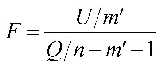
To test whether the regression of the SVR model is significant, we used an F-test. In eqn (7), U is the regression square sum of the modelQ is the sum of the residual square of the model m′ is the number of reserved descriptors, and n is the number of training set samples. If F > F_α(n − m′ − 1), we can assert that the model has significant nonlinear regression at level α (0.01). Furthermore, we used the single-factor effect analysis method to assess the influence trend of the single reserved descriptors on response variable Y.²⁰

7

where y_{test_i} is the experimental value in the test set, 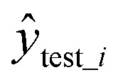is the predicted value in the test set, 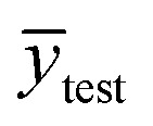is the mean experimental value of the test set, y_train__i is the experimental value in the training set, 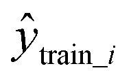is the predicted value in the training set, and 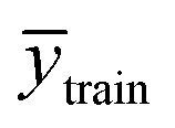is the mean experimental value of the training set.

3. Results and analysis

3.1. Chi-MIC-share feature selection process

After feature selection by Chi-MIC-share, the reserved descriptors of the three datasets were 15, 27, and 22. Fig. 1 displays the selection processes. The redundancy allocation score no longer increases when features were introduced to a certain number.

Fig. 1. Chi-MIC-share scores for three datasets.

3.2. Comparison of feature selection methods

To verify the efficacy of the redundancy allocation concept, we performed feature selection on the three high-dimensional datasets using univariate filter methods R, dCor, Chi-MIC and multivariate filter methods mRMR, Chi-MIC-share. The well-tuned SVR model was used to evaluate the feature subsets refined by feature selection methods. The SVR model used in this paper is derived from the LIBSVM software package (https://www.csie.ntu.edu.tw/∼cjlin/libsvm/index.html). The SVM type is set to epsilon-SVR; the SVR model has three commonly used kernel functions, linear kernel, polynomial kernel, and Radial Basis Function (RBF). Compared with other kernel functions, RBF kernel shows better generalization ability in most cases. Therefore, RBF kernel was used in the experiment. The parameters include penalty parameter c, RBF kernel parameter g, and loss function parameter p. The three parameters were optimized by grid search with 5-fold cross-validation on the training set. The range of each parameter is set according to the software default, and 2 is the base of logarithm, the index range of parameter c is [−1, 6], the index range of parameter g is [−8, 0], and the index range of parameter p is [−1, −8]. Normalize the data to [−1, 1] before training the model to correctly reflect the actual situation of the data.

Since R, dCor, Chi-MIC and mRMR cannot automatically select feature subsets, two heuristic forward selection methods were used to filter the final feature subsets. (a) Introduce one forward feature at a time, and for each feature introduced, 5-fold cross-validation was implemented on the training set by machine learning algorithms such as support vector machine until all features were introduced, and no features were removed in this process. The features with highest accuracy after cross-validation were selected for the optimal feature subset;²⁶ (b) introduce one forward feature at a time, retained those that were useful and eliminated the useless until all features were traversed. In this process, features that cannot improve cross-validation accuracy were eliminated.²⁷ When there are too many features, forward selection methods are time-consuming, so we selected the top 100 features and then performed forward selection methods on the training set.

Table 4 shows that Chi-MIC-share is superior to the reference feature selection methods in all three datasets. There is no obvious difference among the three univariate filter methods because the feature selection process is affected by many factors. First, the univariate screening methods ignore the correlation between features, and at the same time selecting features with strong correlation will lead to deviations in prediction accuracy. Second, heuristic search does not traverse all features, and it is easy to fall into the local optimal. In addition, relying on a learning machine to search for a subset of features may lead to overfitting of training model. The multivariable screening method mRMR does not show advantages over the univariate screening methods, indicating that the redundancy is not removed correctly. Chi-MIC-share considers redundant allocation among features, does not rely on learning machine, and uses a complete search in the feature space. Experimental results show the superiority of this algorithm.

Feature selection and independent prediction accuracy of SVR model.

Methods	Feature number	Dataset 1		Feature number	Dataset 2		Feature number	Dataset 3
		MSE	R 2		MSE	R 2		MSE	R 2
All	1219	0.1066	0.7793	1323	0.1740	0.8389	1360	0.1709	0.7468
R a	19	0.0626	0.8686	65	0.0489	0.9658	91	0.3431	0.4541
R b	20	0.0994	0.8121	18	0.0477	0.9503	37	0.3655	0.4445
dCora	49	0.0948	0.7873	88	0.0283	0.9733	100	0.2358	0.6212
dCorb	15	0.0701	0.8368	42	0.0229	0.9767	25	0.1640	0.7518
Chi-MICa	86	0.0985	0.7842	61	0.0561	0.9467	82	0.2488	0.5975
Chi-MICb	27	0.1387	0.7029	34	0.0791	0.9716	15	0.4184	0.3631
mRMRa	15	0.1339	0.7180	98	0.1088	0.8876	70	0.1686	0.7503
mRMRb	13	0.1291	0.7188	26	0.1139	0.8578	11	0.2968	0.5607
Chi-MIC-share	15	0.0280	0.9590	27	0.0226	0.9750	22	0.0454	0.9367

^aForward selection method without culling feature.

^bForward selection method with culling feature.

3.3. Comparison of the results of this article with references

Due to differences in descriptors and evaluation indicators, we simply compared the results with related published reports. For Dataset 1, the MSE of the present work is 0.0280 and R² is 0.9590; the previously reported values²¹ are 0.0424 and 0.919, respectively. For Dataset 2, we found that R² = 0.9750, and a previously reported value²² is 0.8949. For Dataset 3, we found that R² is 0.9367, and a previously reported value²³ is 0.9197. We can see that our independent predictions of SVR based on Chi-MIC-share are better than those reported in the literature. Fig. 2 shows the distribution of observed values and predicted values for the three datasets, confirming the results.

Fig. 2. Observed values and predicted values of three datasets.

3.4. Model significance test and single-factor effect analysis

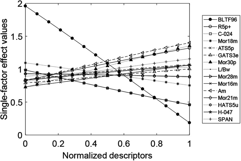
Taking Dataset 1 as an example, the 15 reserved descriptors selected by Chi-MIC-share established the SVR model, F = 21.93 > F_0.01(15, 40) = 2.1076, indicating that the model is significant. Table 5 shows the reserved descriptors and the corresponding group names and explanations, and Fig. 3 shows the single-factor effects of the 15 reserved descriptors in Dataset 1.

Fifteen reserved descriptors in Dataset 1.

Group name	Descriptor name	Explanation
Molecular properties	BLTF96	Verhaar model of algae base-line toxicity from MLOGP (mmol l−1)
3D-MoRSE descriptors	Mor30p	3D-MoRSE-signal 30/weighted by atomic polarizabilities
	Mor16m	3D-MoRSE-signal 16/weighted by atomic masses
	Mor28m	3D-MoRSE-signal 28/weighted by atomic masses
	Mor18m	3D-MoRSE-signal 18/weighted by atomic masses
	Mor21m	3D-MoRSE-signal 21/weighted by atomic masses
Geometrical descriptors	SPAN	span R
	L/Bw	Length-to-breadth ratio by WHIM
WHIM descriptors	Am	A total size index/weighted by atomic masses
Atom-centered fragments	H-047	H attached to C1(sp3)/C0(sp2)
	C-024	R–CH–R
2D autocorrelations	ATS5p	Broto–Moreau autocorrelation of a topological structure-lag 5/weighted by atomic polarizabilities
	GATS3e	Geary autocorrelation-lag 3/weighted by atomic Sanderson electronegativities
GETAWAY descriptors	R5p+	R maximal autocorrelation of lag 5/weighted by atomic polarizabilities
	HATS5u	Leverage-weighted autocorrelation of lag 5/unweighted

Fig. 3. Single-factor effects of the 15 reserved descriptors in Dataset 1.

For the 15 reserved descriptors, the molecular global descriptors are molecular properties, three-dimensional molecule representation of structure based on electron diffraction (3D-MoRSE) descriptors, geometrical descriptors, and weighted holistic invariant molecular (WHIM) descriptors. The molecular local descriptor is atom-centered fragments. Molecular combination descriptors are two-dimensional autocorrelations and geometry, topology, and atom weights assembly (GETAWAY) descriptors. BLTF96 is the n-octanol/water partition coefficient, which is a parameter in measuring the lipophilicity of organic compounds in water. Experiments have shown that the n-octanol/water partition coefficient is strongly correlated with various toxicological properties of compounds.²⁸ Mor30p, Mor16m, Mor28m, Mor18m, and Mor21m^29–34 are atomic polarity parameters and atomic mass parameters; SPAN and L/Bw descriptors³⁵ reflect geometrical features such as molecular surface area, volume, and stereoscopic parameters. H-047 and C-024 ³⁶ highlight the importance of hydrogen and carbon atoms in influencing the negative log half-maximal inhibition growth concentration, as they participate in intermolecular interactions through hydrogen bonds in the solid state. ATS5p and GATS3e^37,38 are vector descriptors that are based on the two-dimensional structure of a molecule and the properties of atomic pairs. R5p+ and HATS5u^39,40 characterize the distribution of atomic properties on a topological structure, which is a combination of geometry, topology, and atomic components. The effects of these parameters on chemical compounds have been reported in the literature.

WHIM descriptors are new three-dimensional molecular property indices, contain information about the molecular structure of a chemical compound in terms of size, shape, symmetry, and atom distribution. Am is the total molecular volume parameter of WHIM descriptors, and our findings demonstrate that its effects cannot be ignored.

Fig. 3 displays the single-factor effect. The factors that are positively correlated with the effects of phenolic compounds on T. pyriformis are Mor30p, Am, R5p+, SPAN, ATS5p, Mor28m, Mor16m, L/Bw, and GATS3e. The factors that are negatively correlated with the effects are BLTF96, H-047, C-024, Mor18m, Mor21m, and HATS5u.

4. Conclusions

When the features of sample contain massive irrelevant or redundant information, the performance of the mathematical model is seriously affected. By constructing more reasonable and reliable correlation or significance metrics, feature selection methods can single out the most suitable feature subset from high-dimensional features, reduce the complexity of the model, avoid over-fitting, and enhance the interpretability of the model. MIC can be used to measure the correlation compactness between variables, has universality and equivalence, and relevant studies have shown its effectiveness.

In this paper, we used the redundancy allocation algorithm with Chi-MIC to automatically filter trusted features, then verified the superiority of redundancy allocation over de-redundancy using experimental datasets. Dynamic calculation of share score is an important part of the chi-MIC-share algorithm. First, it does not rely on the learning machine, but only uses the constructed statistics to filter features. Second, based on the overall features, it comprehensively weighs the change of each feature score in the original set after a new feature is introduced, and the impact of such changes on the entire new set. This dynamic adjustment will prevent the subset score from increasing all the time. When a vertex is reached, the feature selection process is also terminated. This may provide a new idea for quantitative research and has certain reference value.

Conflicts of interest

There are no conflicts to declare.