A novel artificial intelligence protocol to investigate potential leads for Parkinson's disease

Abstract

Previous studies have shown that small molecule inhibitors of NLRP3 may be a potential treatment for Parkinson's disease (PD). NACHT, LRR and PYD domains-containing protein 3 (NLRP3), heat shock protein HSP 90-beta (HSP90AB1), caspase-1 (CASP1) and cellular tumor antigen p53 (TP53) have significant involvement in the pathogenesis pathway of PD. Molecular docking was used to screen the traditional Chinese medicine database TCM Database@Taiwan. Top traditional Chinese medicine (TCM) compounds with high affinities based on Dock Score were selected to form the drug–target interaction network to investigate potential candidates targeting NLRP3, HSP90AB1, CASP1, and TP53 proteins. Artificial intelligence model, 3D-Quantitative Structure–Activity Relationship (3D-QSAR) were constructed respectively utilizing training sets of inhibitors against the four proteins with known inhibitory activities (pIC₅₀). The results showed that 2007_22057 (an indole derivative), 2007_22325 (a valine anhydride) and 2007_15317 (an indole derivative) might be a potential medicine formula for the treatment of PD. Then there are three candidate compounds identified by the result of molecular dynamics.

Three candicates gained by a novel artificial intelligence protocol for Parkinson's disease (PD).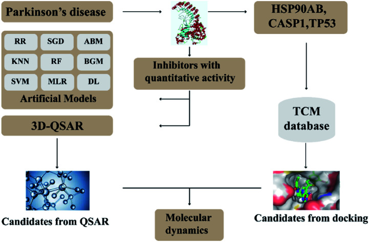

1. Introduction

Parkinson's disease (PD) is a neurological disorder with evolving layers of complexity,¹ which is more common in the elderly. Details regarding the pathophysiological basis of PD has been greatly expanded over the past two decades, with extraordinary contributions from the field of genetics,² however, the exact cause of this pathological change is still unknown.¹ Environmental factors are no longer viewed as only primary risk of the development of PD,¹ genetic factors, environmental factors, aging, oxidative stress and some other factors may be involved in the degeneration and death process of PD dopaminergic neurons.

Previous studies have shown that small molecule inhibitors of NACHT, LRR and PYD domains-containing protein 3 (NLRP3) may be a potential treatment for PD,³ The NLRP3 inflammasome participates in the pathogenesis of PD, and inhibiting the downstream pathway of the NLRP3/caspase-1/IL-1β axis can alleviate the occurrence of PD symptoms,⁴ Inhibition of hepatic NLRP3 inflammasome weakens inflammatory cytokines spreading into the brain and delays the progress of neuroinflammation and DA neuronal degeneration.³

In the past few years, we have developed computer-aided drug design servers.⁵ There are two things enable us to effectively screen new compounds for many diseases. IScreen has been used for conducting online virtual screening and new drug design,⁶ at the same time, ISMART which is based on TCM database (TCM Database@Taiwan),⁷ has been used for computer-aided drug design. Traditional Chinese medicine (TCM) has a long history of viewing an individual or patient as a system with different statuses and has accumulated numerous herbal formulae,⁸ Currently pharmacologic dogma, “single drug, single target, single disease”, is at the root of the lack of drug productivity. From a systems biology viewpoint, network pharmacology has been proposed to complement the established guiding pharmacologic approaches,⁹ Viewing drug action through the lens of network biology may provide insights into how we can improve drug discovery for complex diseases,¹⁰ Molecular docking is a key tool in structural molecular biology and computer-assisted drug design. Docking can be used to perform virtual screening on large libraries of compounds, rank the results, and propose structural hypotheses of how the ligands inhibit the target, which is invaluable in lead optimization,¹¹ Deep learning is beginning to impact biological research and biomedical applications as a result of its ability to integrate vast datasets, learn arbitrarily complex relationships and incorporate existing knowledge.¹² Similarly, random forest can also be applied in biomedicine.¹³ Based on the structure–activity relationship, quantitative structure–activity relationship (QSAR) modeling is the process to reveal the relationship between molecular structure and bioactivity with mathematical theories and different modellers will utilize it in different ways.¹⁴ To be specific, QSAR is try to establish some formulas to describe the relationship between structural properties (like log P) and bioactivities (like pIC₅₀) quantificationally.¹⁵ With the rapid development of computational science and chemistry biology, QSAR is now not only used in predicting physical and chemical properties, but also applied in drug design because of its ability to predict biological properties¹⁶ and because of this, QSAR models are in large use in companies and public services today after experiencing of a long evolution.¹⁶ Combination of artificial intelligence and QSAR models, which will be applied in these research, the accuracy is increased largely.¹⁷ A variety of artificial intelligence methods can be used to build QSAR models, such as multiple linear regression (MLR),¹⁸ support vector machine (SVM),¹⁹ comparative force field analysis (CoMFA) and comparative similarity indices analysis (CoMSIA) models and this model can predict the biological properties of candidates in drug design. It has served as a valuable predictive tool in the design of pharmaceuticals and agrochemicals. Although the trial and error factor involved in the development of a new drug cannot be ignored completely, QSAR certainly decreases the number of compounds to be synthesized by facilitating the selection of the most promising candidates. Several success stories of QSAR have attracted the medicinal chemists to investigate the relationships of structural properties with biological activity.²⁰ Even though QSAR is largely used in this day and age, a lot of concerns about the reliability occur. One of the rules that should be obeyed in QSAR is applicability domain.²¹ Since that the compounds used in this study were all from the same research, most of the descriptors do not show extreme differences and before choosing the training sets and testing sets, we had already made sure that test compounds did not violate the range of maximum and minimum value for descriptors of compounds,²¹ which is one of the reasons that QSAR results are reliable. At the same time, network pharmacology was used to search for target proteins related to Parkinson's syndrome in this study.

In this research, we use molecular docking technology to screen suitable small molecules from the database of Chinese herbal medicines. Several methods such as 2d-QSAR and 3d-QSAR are used to analyze their biological activity. Last but not least, molecular dynamics has been treated as a crucial way to identify the candidate compounds from the database. The specific process is shown in the Fig. 1.

Fig. 1. Flow chart of experimental design.

2. Materials and methods

2.1. Compound-network analysis

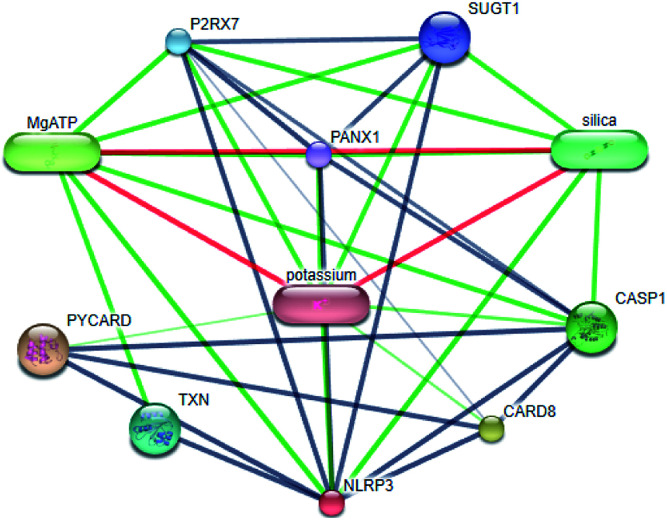
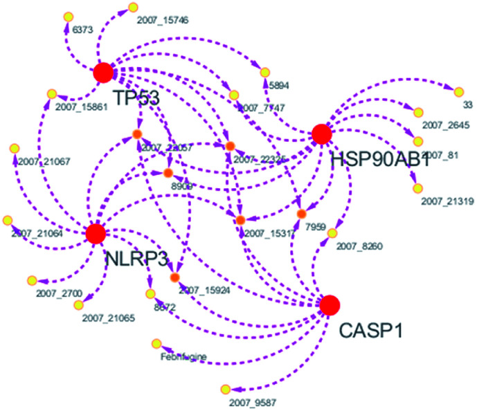
Systems biology suggests that complex diseases may not be effectively treated with the intervention of a single node. Therefore, finding protein pathways and analyzing multiple proteins is an effective method. Protein–protein interactions (PPI) obtained from STRING database (STRING v10.5, http://string-db.org/)²² were used to find proteins associated with NLRP3 and PD. The correlation between related proteins, NLRP3 and PD was scored through a certain scoring function. The top ten proteins and their interactions are shown in Fig. 2. Fig. 3 is constructed by analyzing the interaction relationship between NLRP3, TP53, CASP1, HSP90AB1 which are the four related proteins and molecular in the TCM Database@Taiwan (http://tcm.cmu.edu.tw). This chart can be used to further analyze potential targets for PD and multi-target drugs for PD.

Fig. 2. Network of protein–protein interactions.

Fig. 3. Compound–target network.

2.2. Virtual screening and docking

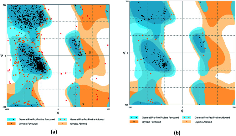
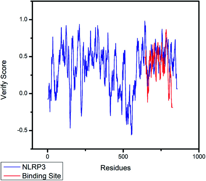
The crystal structures of TP53, CASP1 and HSP90AB1 proteins were obtained from RCSB Protein Data Bank²³ (PDB ID: 2Z21,²⁴1RWX,²⁵5FWK,²⁶ respectively). The sequences of these four proteins were obtained from Uniprot Knowledgebase²⁷ (Identifier: NLRP3-Q96P20, TP53-P04637, CASP1-P29466 and HSP90AB1-P08238, respectively). With I-TASSER242526 (https://zhanglab.ccmb.med.umich.edu/I-TASSER/),^28–30 the crystal structure of NLRP3 was constructed complete protein structure. The complete protein structure contained ligands for predicting binding sites and the highest confidence model was chosen. Ramachandran plot validation of our modelling structure and the 3D-profile validation of modelling structure, which can help us to find whether the structure is reliable, are shown in Fig. 4 and 5, respectively. We used the ‘Prepared protein’ module in Accelrys Discovery Studio (DS) software to prepare the proteins in order to make the result more credible. 18776 TCM compounds from TCM Database@Taiwan (http://tcm.cmu.edu.tw)⁷ which were filtered by Lipinski's rule of five, were applied to dock into NLRP3, TP53, 1RWX, and 5FWK protein structures by using LigandFit module³¹ in DS. To minimized docking poses between ligands and proteins, Chemistry at HARvard Molecular Mechanics (CHARMm) force field^32,33 were used. During the docking process, the DREIDING force field containing Gasteiger charges was chosen to calculate the interaction energy for each ligand. The ADMET descriptors module in DS was used to calculate absorption, distribution, metabolism, excretion, toxicity (ADMET) properties such as solubility, blood–brain barrier (BBB) penetration, hepatotoxicity, cytochrome P450 2D6 (CYP2D6) inhibition, plasma protein binding (PPB) level, and absorption. Results of the docking studied were ranked according to Dock Score which was calculated mainly based on the interaction energy between ligand and protein.

Fig. 4. Ramachandran plot validation of modeling structure. (a) Complete structure, (b) binding site fragment.

Fig. 5. The 3D-profile validation of modeling structure. The verify score which is higher than 0 signifies the trusted simulation of amino acids.

2.3. 2D-QSAR models

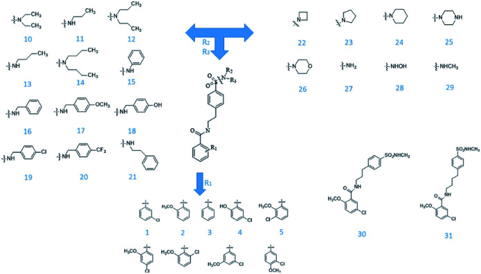
From Jacob Fulp's study,³⁴ we obtained the structures of 31 NLRP3 inhibitors (Fig. 6) and pIC₅₀ value (μM) (Table 1) which included 6 testing set compounds and 25 training set compounds. We drew chemical structures of the compounds by ChemBioDraw software. The activity value of NLRP3 inhibitors was normalized by eqn (1):

pIC₅₀ = 6 − log₁₀(IC₅₀) 1

Fig. 6. The known small molecular structure of NLRP3 inhibitors from previous study.

Activity values (pIC₅₀) of NLRP3 from previous study.

Comp.	pIC50
1	4.874
2	4.765
3	3.834
4	4.981
5	4.498
6	4.744
7	4.352
8	5.234
9	4.485
10	5.699
11	5.785
12	5.854
13	6.013
14	6.260
15	5.686
16	5.883
17	6.377
18	6.201
19	5.824
20	5.721
21	6.081
22	5.780
23	5.478
24	5.301
25	5.469
26	5.463
27	5.488
28	5.073
29	5.487
30	5.693
31	5.759

For improving the accuracy of the result, we regarded pIC₅₀ value as a key property. We calculated molecular descriptors of these compounds in calculate molecular properties in DS and selected 10 properties with the best correlation from 204 properties by removing low correlation ones. The selected properties and pIC₅₀ were used to build 2D-QSAR models respectively. The 2D-QSAR models were used to predict the bioactivities (pIC₅₀) of TCM candidates. Recently, in Kunal Roy's article,³⁵ the potential error in R² based metrics for external validation of QSAR models is mentioned. Thus, after building the QSAR models like SVM, MLR, we checked the MAE based criteria of all QSAR models apart from deep learning, since we applied MSE during the process of building deep learning model.

2.3.1. SVM and MLR models

QSAR models were constructed through SVM¹⁹ and MLR¹⁸ machine learning algorithms which were established in libSVM software and Matlab software.

Through eqn (2), we acquired the SVM model's square correlation coefficient (R²) which represent that SVM is suitable to predict compounds' abilities.

2

At the same time, the MLR model was described by eqn (3):

Y = b₀ + b₁ × X₁ + b₂ × X₂ + … + b₇ × X₇ 3

2.3.2. Deep learning model

In order to improve the accuracy of the prediction results, deep learning method was used to construct a composite activity prediction model.³⁶ The mean square error (MSE) was used as a loss function. The neural network weights were updated using an Adam optimizer with a learning rate of 0.006, and applied other parameters of the original paper to the model. A four-layer fully connected neural network was constructed by correcting the linear unit function as the activation function. The Adam optimizer, which learning rate 0.0001 and other parameters were determined in the original file, was used in this paper. To reduce overfitting, the Dropout technique was applied to the second layer (rate 0.4) and the third layer (rate 0.6) of the neural network.

2.3.3. Random forest model

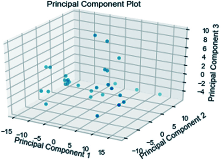
Analogously, this paper also applied a random forest model. The relationship between the 204 properties calculated by GFA algorithm was analyzed using the Pearson correlation coefficient matrix. The results are represented by the Python package Yellowbrick as a picture. Principal component analysis (including 2D and 3D)³⁷ was used to analyze the relationships between attributes for the 31 composite data set. Pre-processing of the data set included the following steps. To begin with, we amplified the numerical values of the properties to between 0 and 1 and then selected 54 properties with a variance greater than 0.05. Furthermore, we normalized and got the data with a mean of 0 and a variance of 1. In the end, we got nine properties using lasso feature selection. The Pearson correlation coefficient matrix heatmap of these nine properties showed that the research results were credible.

2.3.4. Ridge regression model

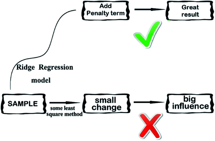
Ridge regression,³⁸ is a dedicated to total linear biased estimation of regression data analysis method, in essence, is a kind of improved least squares estimation method by giving up the unbiasedness of least-square method. Losing some information to reduce the accuracy at the expense of regression coefficient is more practical, more reliable regression method, the fitting of pathological data than the least square method. Ridge regression model is a widely used model.³⁹ Ridge regression is to artificially add a non-negative factor k to the main diagonal elements of the information matrix composed of independent variables, so that the matrix determinant is not zero, to reduce the error of regression coefficient estimation, improve the estimation accuracy and the model stationarity. Ridge regression can repair the ill-conditioned matrix and achieve better results. Its simplified diagram is shown in Fig. 7.

Fig. 7. A simplified diagram of the ridge regression model.

2.3.5. Stochastic gradient descent model

Aiming at the disadvantage of slow training speed of BGD algorithm, SGD algorithm is proposed. The common BGD algorithm is to pass all samples once per iteration and update the gradient once for each training group of samples. SGD algorithm randomly extracts a group from samples, updates it once according to gradient after training, and then extracts another group and updates it again. In the case of an extremely large sample size, it may not need to train all samples to obtain a model with acceptable loss value. The core of stochastic gradient descent is: gradient is an expectation. Small sample estimates are expected. Specifically, in each step of the algorithm, we evenly extract a small batch of samples from the training set B = {x(1), …, x(m′)}. The number of small batches m′ is usually relatively small, ranging from one to several hundred. Importantly, m prime is usually fixed as the size of the training set increases. We are probably fitting billions of samples, and we're only using a few hundred samples per update.

2.3.6. Elastic net model

Elastic network⁴⁰ is a linear regression model using L1 and L2 norm as prior regular term training. This combination allows you to learn a non-zero sparse model with a few parameters, like lasso, but it still retains some regular properties like ridge. The convex combination of L1 and L2 can be controlled by the l1_ratio parameter. Elastic networks are an iterative method. The best thing about elastic networks is that they can always produce efficient solutions. Because it doesn't cross paths, the solutions are pretty good. But the most attractive thing about elastic networks is not their efficient solution, but their rate of convergence. Elastic networks are very useful when many features are linked. Lasso is likely to consider only one of these features at random, while elastic networks prefer two. In practice, one advantage of the tradeoff between lasso and ridge is that it allows the ridge stability to be inherited under rotate.

2.3.7. Bagging model

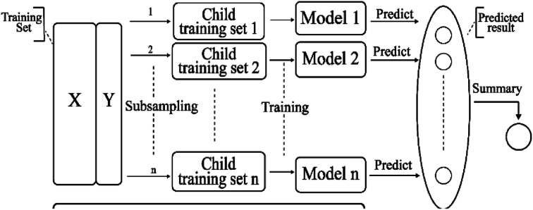
Bagging⁴¹ is also known as a bootstrap aggregating method, where T new data sets are obtained after the initial data sets are selected for T times. Obtained by putting back a sample (for example, to get a new data set of size n, each sample of which is sampled randomly from the original data set, i.e., after sampling and putting back). Based on each sampling and training, a basic learner is trained, and then these basic learners are combined. When combining the predicted output, bagging usually adopts a simple voting method for classification tasks and a simple average method for the regression task. Bagging focuses on reducing variance. The algorithm is as follows: (A) the training set is extracted from the original sample set. N training samples are harvested per round from the original sample set using the bootstrapping method (in a training set, some samples may be harvested multiple times while others are not harvested at all). A total of m rounds was extracted to obtain m training sets (k training sets are independent of each other). (B) A model is obtained by using one training set at a time, and a total of m models are obtained by using m training sets (note: there is no specific classification algorithm or regression method here, we can adopt different classification or regression methods according to specific problems, such as decision tree, perceptron, etc.). (C) classification: the m models obtained in the previous step are voted to get classification results. For regression problem, the mean value of the above models is calculated as the final result (all models are equally important). Its simplified diagram is shown in Fig. 8.

Fig. 8. A simplified diagram of the bagging model.

2.3.8. k-Nearest neighbor model

k-Nearest neighbor (KNN)⁴² works, is a sample data set, also known as a training sample set, and each data in the sample set has a label, that is, we know the relationship between each data in the sample set and its classification. After data without labels are input, each feature in the new data is compared with the corresponding feature of the data in the sample set, and the classification label of the data with the most similar feature (nearest neighbor) in the sample set is extracted. Generally speaking, we only select the first k most similar data in the sample data set, which is where k comes from in the k-nearest neighbor algorithm and k is an integer less than 20. Finally, the classification with the most occurrence of k most similar data is selected as the classification of the new data. KNN does not show the training process, which is the representative of “lazy learning”. It only saves the data in the training stage, and the training time is 0, which will be processed after receiving the test samples.

2.4. 3D-QSAR model (CoMFA and CoMSIA analysis)

Based on the three-dimensional structure characteristics of drug molecules and receptor molecules, 3D-QSAR is a method to analyze the quantitative relationship between structure and biological activity. We divided 31 NLRP3 inhibitors with similar skeletons from Jacob Fulp's study⁴³ into 25 for the training set and 6 for the testing set to do 3D-QSAR analysis. The 3D QSAR model was constructed using SYBYL-X 1.1. By partial least squares (PLS), we established the comparative force field analysis (CoMFA) and comparative similarity index analysis (CoMSIA) models. In order to establish appropriate 3D-QSAR model, we need to align the training set molecules, and use atomic fitting module. The cross-validation correlation coefficient (CV) greater than 0.4 and the model with a non-cross-validation correlation coefficient (R²) greater than 0.8 is considered to be reliable. Through 3D-QSAR contour map, we can predict the biological activity of the control and Chinese medicine candidates.

2.5. Molecular dynamics simualtion

In order to verify the stability of the compound–protein complexes from the docking study, in this study, we used GROMACS^44,45 to do molecular dynamic simulation (MD). Firstly, from Swissparam web server,⁴⁶ we obtained topology files and parameters for the ligands. Placed in a periodic cubic box with a 1.2 nm edge, the protein–ligand complex was solvated with TIP3P water molecules and 0.145 M NaCl ions. The complex systems were minimized for 5000 steps by the steepest descent algorithm. The temperature was set at 310 K in the canonical ensemble (NVT) and isothermal–isobaric ensemble (NPT). The NVT balance simulation is a total of 20 ns with a time step of 2 fs. The Lincs algorithm constrains all keys and 310 K temperature settings, similar to the physiological environment. The NPT operates in balance for 20 ns and sets the temperature coupling during the simulation.

PBC for periodic boundary conditions were performed with Verlet scheme in this 100 ns dynamic simulation. For analyzing the stability of the compound–protein complexes, we calculate root mean square deviation (RMSD), total energy, the radius of gyrate, solvent-accessible solvent area (SASA), root mean square fluctuation (RMSF), mean square deviation (MSD).

3. Results and discussion

3.1. Compound-network analysis

We have a better way to explore the molecular mechanisms of disease and the ultimate treatment in the past years for the reason that many researchers have obtained a large number of data on PPI, which are important components of cellular signaling, play a crucial part in the pathogenesis of many diseases in a variety of forms. Through the STRING10 website, we constructed a PPI network to better target the target proteins of Parkinson's syndrome and then search for drugs from the Chinese herbal medicine database based on these target proteins. Through protein interaction analysis, the resulting proteins are ranked by interaction scores. Scores and rankings are shown in Table 2, and from it, many high-scoring proteins can be seen. Among these proteins, we studied the study of each protein. Several studies, NLRP3, TP53, HSP90AB1, which have a relatively large number of 3D structures on PDB, are thought to be associated with Parkinson's syndrome. Then we used the small molecules in the TCM database to dock the four proteins. More than forty small molecules and corresponding proteins in the top ten of the four proteins in the docking score were used to construct the drug and protein, and action diagram has been shown in Fig. 3. It can be seen that most of the small molecules with high affinity for NLRP3 are also related to the other three proteins, which suggested that NLRP3 can be used as a target for finding drugs for potential PD.

PPI associated with NLRP3.

node1	node2	node1_string_internal_id	node2_string_internal_id	combined_score
HSP90AA1	FKBP4	1851814	1842112	0.999
HSP90AB1	CDC37	1850780	1842879	0.999
TXN	MAP3K5	1856133	1853780	0.999
AR	UBC	1856164	1852861	0.999
HSP90AA1	ERBB2	1851814	1846101	0.999
HSP90AA1	NR3C1	1851814	1843294	0.999
HSP90AA1	AKT1	1851814	1846136	0.999
HSPA8	STUB1	1843112	1842759	0.999
HSP90AA1	RAF1	1851814	1844086	0.999
HIF1A	TP53	1852062	1846083	0.999
TP53	STUB1	1846083	1842759	0.999
HSP90AB1	STIP1	1850780	1848791	0.999
UBC	AKT1	1852861	1846136	0.999
FAF1	UBC	1855550	1852861	0.999
SUGT1	HSP90AB1	1856790	1850780	0.999
HSP90AA1	CDC37	1851814	1842879	0.999
CASP1	NLRC4	1860827	1854083	0.999

3.2. Virtual screening

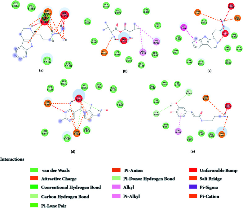
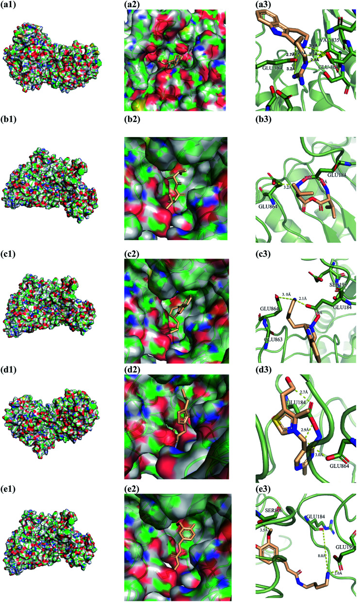
From the compound–target interaction network constructed by analyzing the docking results, 2007_22057, 2007_22325, 2007_15317, 8909, 7959 were selected, because these five Chinese herbal medicines simultaneously obtained higher scores with NLRP3, CASP1, TP53 and HSPAB1, which indicated that they have a high binding affinity with these four proteins. Due to CASP1, TP53 and HSPAB1 lacked relevant data for the study, NLRP3 protein was used as a key protein for further research. Compound 17, which was obtained from Jacob Fulp's study, was selected as the control for the reason that it showed good biological activity in medicinal chemistry experiments. 2D diagram of the combined pattern in five target complexes is shown in Fig. 9. Based on the docking pose of NLRP3 in Fig. 10, the amino cation of 2007_22057 formed a hydrogen bond (2.1 Å) with GLU184 of NLRP3 and a hydrogen bond (3.4 Å) with GLU864 of NLRP3. The tertiary carbon of 2007_22057 formed a hydrogen bond (2.7 Å) with GLU184 of NLRP3. The amino cation with the double bond of 2007_22057 formed a hydrogen bond (3.2 Å) with GLU184 of NLRP3. The tertiary amino of 2007_22057 formed a hydrogen bond (2.8 Å) with GLU864 of NLRP3. The secondary carbon of 2007_22057 formed a hydrogen bond (3.3 Å) with GLU864 of NLRP3. The amino cation of 2007_22325 formed two hydrogen bonds (1.7 Å and 1.7 Å) with GLU184 of NLRP3. The amino cation of 2007_22325 formed a hydrogen bond (3.2 Å) with GLU864 of NLRP3. The amino cation of 2007_15317 formed a hydrogen bond (2.1 Å) with GLU184 of NLRP3 and a hydrogen bond (3.0 Å) with GLU864 of NLRP3. The imino group of 2007_15317 formed a hydrogen bond (1.8 Å) with GLU184 of NLRP3. The amino cation of 7959 formed a hydrogen bond (2.0 Å) with GLU197 of NLRP3 and a hydrogen bond (8.0 Å) with GLU184 of NLRP3. The amine methyl of 7959 formed a hydrogen bond (3.5 Å) with SER806 of NLRP3. The ether carbon of 8909 formed a hydrogen bond (2.7 Å) with GLU184 of NLRP3. The amino methylene of 8909 formed a hydrogen bond (2.9 Å) with GLU184 of NLRP3 and a hydrogen bond (3.0 Å) with GLU864 of NLRP3. The docking result is shown in Table 3. The chemical scaffold of TCM candidates based on docking and controls is shown in Fig. 11. As shown in Fig. 11, these candidates have diverse chemical structures, like indole structure, valine structure, and so on. Based on the principle of molecular docking, a range of chemical structures in results may indicate that the docking site of the target protein (NLRP3) may be suitable to a lot of basic chemical structure, which is a compelling fact to drug design. In their search for inhibitors,⁴⁷ some crucial structures are significant in drug design, which can also be called lead compounds. Target protein will form a large variety of interactions with compounds, including van der Waals' force, π–π interaction, and so on. Those interactions are based on the structure of target protein and compounds, and the more interactions between them, the better activity it will be.

Fig. 9. 2D diagram of combined pattern in five targets complexes. (a) 2007_22057, (b) 2007_22325, (c) 2007_15317, (d) 8909 and (e) 7959.

Fig. 10. Docking pose of (a) 2007_22057, (b) 2007_22325, (c) 2007_15317, (d) 8909 and (e) 7959 with NLRP3. In (3), the yellow dash lines stand for H-bonds.

Docking results of the control and top ten TCM candidates of PERK ranked by Dock Score^a.

Name	Dock Score	−PLP1	−PLP2	−PMF
2007_22057	209.762	13.73	19.96	85.89
2007_15317	209.502	23.28	29.46	96.3
2007_22325	111.297	1.69	17.93	58.46
8909	193.926	−0.01	13.57	50.82
7959	148.335	33.7	37.23	112.87

^aPLP: Piecewise Linear Potential. PMF: Potential of Mean Force.

Fig. 11. The chemical structure of TCM candidates and controls.

In these results, candidates share diverse chemical structures, which means that there may be a lot of potential lead compounds for the discovery of inhibitor to NLRP3. To verify these results, more experiments including in vitro experiment will be done to test their bioactivities in the future.

The predicted ADMET descriptors are shown in Table 4. ADMET is a significant component in drug design research.⁴⁸ The log S reflect the solubility, and the optimal range is higher than −4 log mol L⁻¹. The result indicated that the solubility of 2007_22057 and 2007_15317 should is excellent. log P means oil–water partition coefficient. Moderate value in log P is suitable for drug to be absorbed into body and the optimal range is 0–3. As shown in Table 4, the log P value of 2007_22057 and 2007_22325 is not belong to optimal range. It may because they are in protonated from, so deprotonation may increase their activity. Absorption of these candidates are compelling. BBB can predict the permeability into brain of candidates. The result indicated that these compounds were suitable to penetrate into brain, which is a gorgeous property for potential PD drugs. Reflecting metabolism characteristic, whether these compounds will inhibit CYP2D6 is predicted. Those compounds which are also the inhibitors of CYP2D6, like 2007_22057, 2007_15317 should concern the interaction between drugs at the same time. Last but not least, all these compounds may not show hepatotoxicity.

The predicted ADMET descriptors of three candidates^a.

Name	log Sa	log P	Absorptionb	BBBc	CYP2D6d	Hepatotoxicitye
2007_22057	−2.257	−1.228	0	1	1	0
2007_15317	−2.369	0.741	1	1	1	0
2007_22325	−1.412	−1.411	0	1	0	0

^alog S: S's unit is mol L⁻¹.

^bAbsorption: good absorption = 0; moderate absorption = 1; low absorption = 2.

^cBBB (Blood Brain Barrier): very high penetration = 0; high penetration = 1; medium penetration = 2; low penetration = 3; undefined penetration = 4.

^dCYP2D6: non-inhibitor = 0, inhibitor = 1.

^eHepatotoxicity: non-inhibitor = 0, inhibitor = 1.

3.3. 2D-QSAR models

3.3.1. SVM and MLR models

When we built property–activity relationship models, the molecular properties that are the same for almost all the molecules are first removed. Then ten molecular properties with large numerical differences between molecules are considered to be a good description of molecules. The 10 properties are A log P, ES_Sum_ssCH2, Dipole_mag, Dipole_X, Jurs_DPSA_1, Jurs_PPSA_3, Jurs_RNCS, IAC_Total, Kappa_3_AM, ES_Sum_aaCH. A log P is the log of the ratio of the partition coefficients of a substance in n-octanol (oil) to water. It reflects the distribution of matter in oil and water phase. ES_Sum_ssCH2 represents the electro topological state (E-state) count for CH₂ with two single bonds. Dipole_mag means the dipole moment. Dipole_X is 3D electronic descriptor that indicates the strength and orientation behavior of a molecule in an electrostatic field Jurs_DPSA_1 on behalf of partial positive solvent reachable surface area minus partial negative solvent reachable surface area. Jurs_PPSA_3 means the sum of the solvent-accessible area of all positively charged atoms in a molecule and their partial charges. Jurs_RNCS represents the solvent-accessible surface area of most negative atom divided by the relative negative charge. IAC_Total property indicates total information of atomic composition. Kappa shape index is a topological index used to characterize molecular shapes. ES_Sum_aaCH represents the electro topological state (E-state) count for tertiary carbon with two aromatic bonds. The MLR model was described in:pIC₅₀ = 10.2930–0.3937 × A log P + 0.0044 × ES_Sum_ssCH2 + 0.0853 × Dipole_mag − 0.0073 × Dipole_X + 0.0014 × Jurs_DPSA_1 – 0.0239 × Jurs_PPSA_3 − 0.1298 × Jurs_RNCS − 0.0568 × IAC_Total + 0.5199 × Kappa_3_AM − 0.0639 × ES_Sum_aaCH

All of the training set and test set molecules were scored using these ten properties to construct a predictive model of biological activity for each molecule in the TCM database. The accuracy of the SVM and MLR model predictions has been verified. The verification results show that both models have high prediction accuracy. It can be seen from the high values of the correlation coefficient (R²) of the SVM model (R² = 0.7925) and the MLR model (R² = 0.8942) that the two models have higher prediction accuracy. Therefore, we used the SVM and MLR models to predict the biological activity of compounds from the Chinese medicine database.

3.3.2. Deep learning model

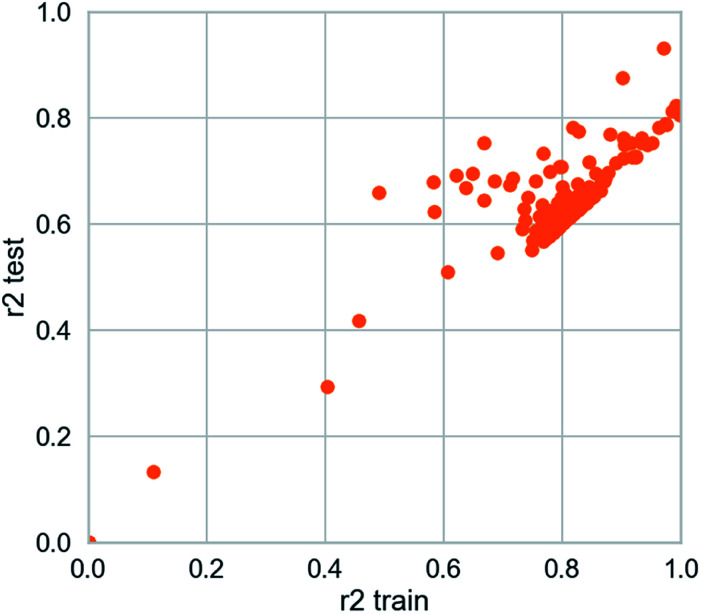
The deep learning method is applied. The training set R² is 0.927 and the test set R² is 0.862. It is studied by a simple four-layer fully connected neural network (Fig. 12). Rectified linear unit (ReLu) was regarded as the activation function. We have fewer training samples. In neural network training, the trained models are likely to overfitting. Dropout can be used as a skill in training deep neural networks. In every training batch, if part of the feature detector is ignored (i.e., making the value of the partially hidden layer node 0), overfitting can be reduced. We used the dropout technique in the second and third layers (the second layer a yield is 0.4), the first three layers of 0.6 to reduce overfitting. Then mean-square error (MSE) is the loss function. The Adam optimizer whose per parameter is well explained is appropriate for unstable objective functions and usually requires little or no adjustment. Learning rate of the Adam optimizer was set to 0.0001 and 120 different attempts was performed and we obtained credible results.

Fig. 12. Scatter plot from deep learning modeling.

3.3.3. Random forest model

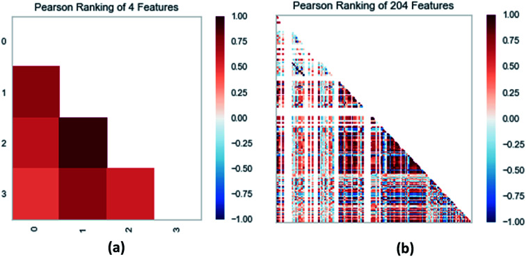
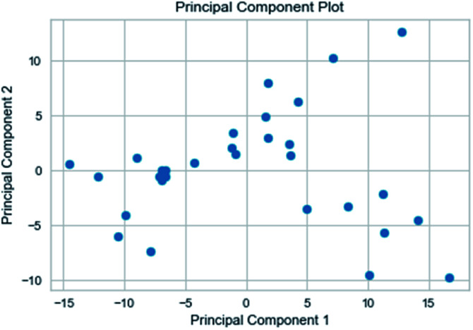
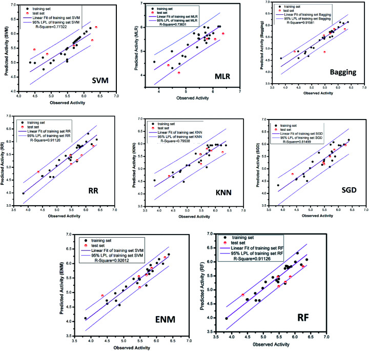
Random forest has excellent accuracy. Our data set includes two interrelated parts, drug activity values and 204 eigenvalues, which led to a higher dimensional data analysis. Samples with high dimensional features can be processed by random forest and it can assess the importance of each feature in the classification problem. The credibility of the study will be increased on account of the obtained high correlation eigenvalues. The Pearson correlation coefficient ranking results show that the correlation coefficient between some features is greater than 0.4 (Fig. 13). The principal component analysis was adopted in this study. Principal component analysis has no effect when the original variables are orthogonal to each other, so there is no correlation between the variables. The results of two-dimensional principal component analysis (2D PCA) and three-dimensional principal component analysis (3D PCA) show that dimensionality reduction makes it easy to find representative features (Fig. 14 and 15). The 204 features were scaled, and the features with variance greater than 0.05 were eliminated to obtain the most representative features. The lasso regression model was used to further screen out nine features with low correlation and good orthogonality. Convert the strongly related variables to as few new variables as possible to replace the original variables. These new, unrelated variables represent various information in the original variables for high-dimensional data processing purposes. In the end, we got the model with the training set mean square error of 0.005 and R-squared of 0.77 (Fig. 16). We believe that the predictions are credible.

Fig. 13. (a) Pearson correlation coefficient matrix heat map of three selected features. (b) Relation of 204 features ranked by Pearson correlation coefficient.

Fig. 14. 2D PCA visualizations.

Fig. 15. 3D PCA visualizations.

Fig. 16. AI models for NLRP3 respectively. The SVM and MLR models identify relationships between observed and predicted activity (pIC₅₀). Correlation trend (purple lines) and 95% prediction confidence regions (enclosed by red lines) are presented. Training set (black dots) and testing set (red dots) are shown. Correlation coefficients (R²) of the QSAR models were all higher than 0.70.

3.3.4. RR, SGD, EN, KNN and bagging models

The ridge regression, stochastic gradient descent, bagging, k-nearest neighbor and elastic network models, which used the same feature selection method as random forest, all had excellent results. The mean square error of RR, SGD, bagging, KNN and ENM are 0.028, 0.070, 0.039, 0.070 and 0.028, respectively. The R-square respectively reach 0.91, 0.81, 0.92, 0.80, 0.93. The candidate activity prediction results obtained from the above five models are mostly superior to the control set (Table 5).

Activity value of candidates and control molecule was predicted by QSAR models.

Name	Predicted value (pIC50)
	SVM	MLR	RF	DL	RR	ENM	SGD	Bagging	KNN
2007_22057	7.639	6.192	5.982	5.918	5.899	5.763	5.548	5.731	5.821
2007_15317	7.693	9.105	5.732	5.205	5.639	5.297	5.366	5.483	5.557
2007_22325	7.894	9.547	4.624	5.167	4.413	4.302	4.745	4.701	4.716
8909	8.314	6.806	5.420	5.619	5.345	5.352	5.336	5.446	5.264
7959	8.069	8.732	5.304	4.859	5.710	5.328	4.826	5.262	5.065
17	6.227	5.739	6.563	6.039	6.298	6.556	6.288	5.875	5.942

The MAE based criteria were conducted after building those QSAR models. In MAE based criteria, SGD, KNN and ENN models were regarded as “good predictions” based on the method in KunalRoy's article.³⁵ All in all, with R² based metrics and MAE metrics, the results of QSAR models are reliable enough.

3.4. 3D-QSAR model (CoMFA and CoMSIA analysis)

Model showed good credibility with a high R² (>0.8), high q² (>0.4), comparatively low SEE and relatively high F values were built from the entire molecular space field and electrostatic field and it can be used to predict the biological activity and visualize favorable and unfavorable characteristics. The first-rank CoMSIA model of NLRP3 (Table 6) consisted of hydrophobic filed (0.692), and hydrogen bond acceptor (0.308). In CoMFA model, there is only one single factor steric field, with the proportion of the electrostatic field is 0. For the CoMFA model, the cross-validation correlation coefficient (q²) and the non-cross-validation correlation coefficient (R²) under different optimal component numbers (ONC) are both greater than 0.4 and 0.9, indicating a reliable confidence level.

CoMFA and CoMSIA models constructed from 31 known NLRP3 inhibitorsa.

Model	q cv 2	R 2	SEE	F	C	S	H	D	A
CoMFA	0.432	0.936	0.153	43.638	6
CoMSIA
S	0.337	0.838	0.236	19.627	6	1
H	0.509	0.917	0.168	42.213	6		1
D	0.044	0.571	0.384	5.055	6			1
A	0.004	0.560	0.389	4.846	6				1
S + H	0.425	0.915	0.171	40.988	6	0.350	0.650
S + D	0.276	0.841	0.234	20.057	6	0.394		0.606
S + A	0.373	0.864	0.222	19.022	6	0.547			0.453
H + D	0.400	0.933	0.156	41.631	6		0.603	0.397
H + A*	0.511	0.914	0.177	31.884	6		0.692		0.308
D + A	0.007	0.622	0.370	4.945	6			0.640	0.360
S + H + D	0.410	0.935	0.153	43.484	6	0.234	0.452	0.314
S + H + A	0.471	0.917	0.174	33.053	6	0.269	0.495		0.236
S + D + A	0.259	0.860	0.225	18.475	6	0.376		0.343	0.281
H + D + A	0.321	0.925	0.165	37.117	6		0.401	0.417	0.182
S + H + D + A	0.408	0.934	0.155	42.529	6	0.207	0.388	0.238	0.167

^a q _cv ²: correlation coefficient (cross validation), R²: correlation coefficient (non-cross validation), C: optimal number of components, SEE: standard error of estimate, F: F-test value, S: steric, H: hydrophobic, D: hydrogen bond donor, A: hydrogen bond acceptor, * selected CoMSIA model filed proportion: H: 70.8%; D: 30.8%; CoMFA model filed proportion: steric field: 100%; electrostatic: 0%.

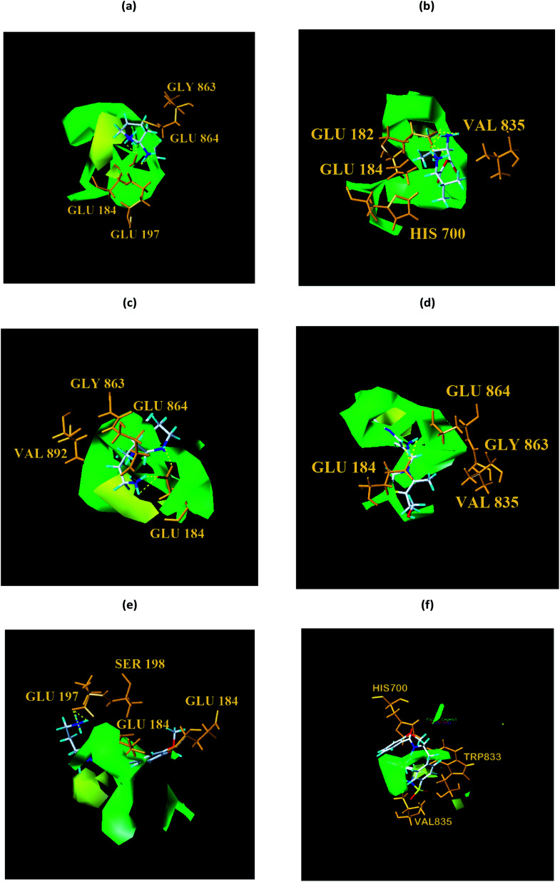
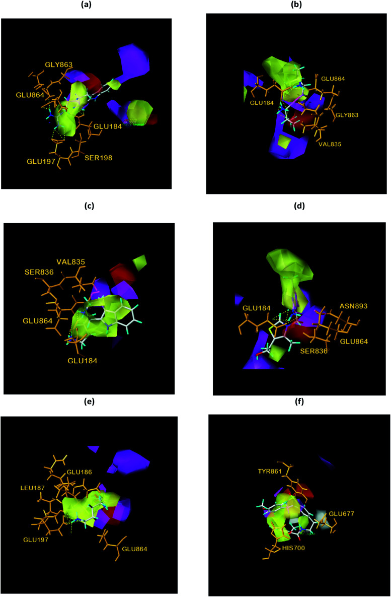
We respectively superimposed CoMFA and CoMSIA contour maps on the control and TCM candidates. CoMFA analysis of NLRP3 is shown in Fig. 17, the compound 17 and the other four candidates of the bulky rings are located in the spatially dominant area (green), and almost no large groups appear near the unpopular (yellow) Chinese medicine candidate area. After mapping the CoMFA contours, the Chinese medicine candidate may have a higher biological activity than the control, which is consistent with the docking results. For CoMSIA analysis of NLRP3 (Fig. 18), after mapping the CoMSIA contours, the Chinese medicine candidate may have a higher biological activity than the control, which is consistent with the docking results. At the same time, it can be seen from CoMFA and CoMSIA contour maps that the number of hydrogen bonds bound to NLRP3 by the four candidates is significantly higher than that of compound 17, which further proves that the activity of Chinese medicine candidates may be stronger than the control. Partial regression leverage plots of 3D-QSAR is shown in Fig. 14.

Fig. 17. Structural contouring of TCM candidates and NLRP3 control to CoMFA mapping. (a) 2007_22057, (b) 2007_22325, (c) 2007_15317, (d) 8909, (e) 7959, (f) 17. The yellow dotted line indicates a hydrogen bond.

Fig. 18. Structural contouring of TCM candidates and NLRP3 control to CoMSIA mapping. (a) 2007_22057, (b) 2007_22325, (c) 2007_15317, (d) 8909, (e) 7959, (f) 17. The yellow dotted line indicates a hydrogen bond.

All in all, the CoMFA and CoMSIA models prove that the candidates not only bound with the protein but also have excellent biological activity.

3.5. Molecular dynamics simulation

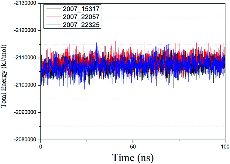
We performed molecular dynamics simulations of target proteins and three candidates up to 100 ns long. The results show that the complex formed by combining the three ligands with the target protein is stable, which further indicates that the three ligands could be candidates for the target protein. We calculated the energy changes in the 100 ns process (Fig. 19), analyzed the energy changes in the complex during the simulation process, and the results show that the ligand–target protein interaction is in an appropriate state. For the complexes of NLPR3 protein and its three candidates, the total energy of the whole simulation is about −2115 000 to −2100 000 kJ mol⁻¹.

Fig. 19. Total energy changes during molecular dynamics simulations between NLRP3 and three candidates. Different colors represent different molecular candidates.

Root mean square deviation (RMSD) was also calculated to study the binding stability of the target protein to the receptor. As shown in Fig. 20(a), RMSD values of the three ligands and target protein complexes all increase around 0–15 ns, and then tended to stabilize with a very stable curve. The RMSD variation of 2007_22057 with the target protein complex is larger than that of the other two ligands. The results show that during the period of 0–15 ns, the ligand binds to target protein, leading to significant changes in RMSD value, after which RMSD value tends to be stable, indicating that the complex has good stability. As shown in Fig. 20(b), the RMSD change curve of the protein is similar to the RMSD change curve of the complex, while the RMSD change curve of the ligand (Fig. 20(c)) is different from the other two change curves, possibly because the RMSD value of the ligand is lower, contributing less to the RMSD value of the complex.

Fig. 20. RMSD changes during molecular dynamics simulations between NLRP3 protein with three candidates. Different colors represent different molecular candidates. (a) RMSD changes of complex, (b) RMSD changes of protein, (c) RMSD changes of ligand.

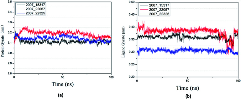
Protein compactness changes can be expressed by calculating gyrate. The gyrate value measures the distance of the atom relative to each center of mass. The smaller the value, the smaller the rotation change, indicating that during the simulation process, the denser the complex. In general, the rate of rotation tends to decline. It can be seen from Fig. 21(a) that the three ligands and target proteins are in the simulation process, and the gyrate of the proteins is stable after 20 ns, while the gyrate is not significantly changed during the whole simulation process, indicating that the stability of the complex is good. Moreover, the gyrate of the protein show a decreasing trend after 80 ns, indicating that the structure is tightened. It can be seen from Fig. 21(b) that the gyrate of the three ligands in the simulation process is more complicated than that of the protein, but the value is smaller, which has little influence on the whole.

Fig. 21. Gyrate result of target complex with three candidates. Different colors represent different molecular candidates. (a) Gyrate result of protein, (b) gyrate result of ligand.

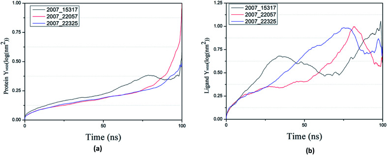
By calculating MSD, we can judge the changes between the initial state and the final state of the protein and ligand, which shows the movement trend of each ligand or protein. The lower the MSD value, the higher the stability of the complex. On the contrary, the higher the MSD value, the lower the stability of the complex. And the rise of MSD values show that ligand has a tendency to escape, as shown in Fig. 22(a), in the process of the whole simulation, the combination of three ligands and protein MSD values continue to rise, and it indicates that all the three ligands have certain escape tendency. In addition, the decrease of MSD value of three ligands at the final stages of simulation indicates that three ligands have a stable trend (Fig. 22(b)).

Fig. 22. MSD results of target complex with three candidates. Different colors represent different molecular candidates. (a) MSD result of protein, (b) MSD result of ligand.

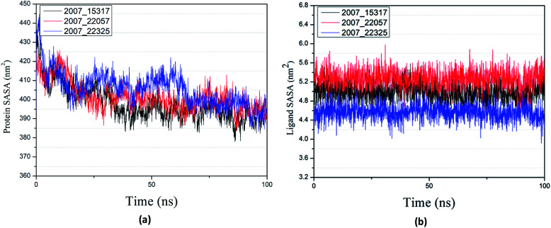
Through SASA analysis, we can understand the hydrophobicity and surface state of proteins. As shown in Fig. 23(a), the SAS value of proteins tends to be stable after the first decline. It can be seen in Fig. 23(b) that the SASA values of all ligands are very stable in the simulation process. This can further determine the stability of the complex.

Fig. 23. SASA result of target complex with three candidates. Different colors represent different molecular candidates. (a) SASA result of protein, (b) SASA result of ligand.

Through RMSF analysis, we can detect the fluctuation of each residue and understand the changes of key residues during the simulation. The average structure of a protein is an average set of atomic coordinates. From Fig. 24, we can see the RMSF value of each protein residue during the simulation of the three ligands and proteins. The higher the RMSF value, the greater the variation of the residue during the simulation.

Fig. 24. RMSF value of each residue on various protein. The abscissa is the number of protein residue sequences. (a) 2007_15317, (b) 2007_22057, (c) 2007_22325.

The average structure of the three ligands and proteins in the simulation process was superimposed with the corresponding final state structure (Fig. 25) to observe whether the two structures were similar, to determine the stability of the complex bound to the target protein. Our RMSD values were 1.341, 0.952, and 1.388, respectively. This indicates that the three ligand–target protein binding complexes have good stability in the simulated final state.

Fig. 25. Average structure of each proteins reacted with different ligands. The average structure and the final state structure are superimposed to obtain RMSD values, and these structures were to observe whether their conformational changes were consistent, which indicate that the final state structure has good stability. (a) 2007_15317, (b) 2007_22057, (c) 2007_22325. (The ligand is not shown in figure.).

Finally, the initial and final states of ligand and target proteins in the simulation process are shown in Fig. 26. The ligand stays in the same pocket of the target protein throughout the simulation.

Fig. 26. Combining posture changes during MD in microenvironment. Although the state of the ligand changes, the position where the ligand binds to the target protein does not change. (a) 2007_15317, (b) 2007_22057, (c) 2007_22325.

4. Conclusions

Through network pharmacology and molecular docking analysis, the small molecules 2007_22057, 2007_22325 and 2007_15317 in the Chinese medicine databases are considered to be able to interact well with NLRP3, a protein associated with Parkinson's syndrome, and to interact with NLRP3-related protein HSP90AB1, CASP1 and TP53. Therefore, these small molecules are selected as candidates for further studies. The artificial intelligence method was used to predict the biological activity of these candidates. After that, we simulated the molecular dynamics of three small molecule candidates and the target protein NLRP3. The results show that the candidate and the target protein bind stably, further explaining the three small molecules could be candidates for the treatment of PD. Given the factors we have just outlined, we think 2007_22057, 2007_22325, 2007_15317 can be regarded as potential molecules for the treatment of PD.

Abbreviation

NLRP3

NACHT, LRR and PYD domains-containing protein 3

DNN

Deep neural network

HSP90AB1

Heat shock protein HSP 90-beta

CASP1

Caspase-1

TP53

Cellular tumor antigen p53

PD

Parkinson's disease

TCM database

Traditional Chinese medicine database

QSAR

Quantitative structure–activity relationship

IC₅₀

Half maximal inhibitory concentration

DL

Deep learning

RF

Random forest

MLR

Multiple linear regression

SVM

Support vector machine

CoMFA

Comparative force field analysis

CoMSIA

Comparative similarity indices analysis

PPI

Protein–protein interaction

CHARMm

Chemistry at HARvard Molecular Mechanics

ADMET

Absorption, distribution, metabolism, excretion, toxicity

BBB

Blood–brain barrier

CYP2D6

Cytochrome P450 2D6

PPB

Plasma protein binding

MSE

Mean square error

RR

Ridge regression

SGD

Stochastic gradient descent

ENM

Elastic net model

KNN

k-Nearest neighbor

CV

Correlation coefficient

RMSD

Root mean square deviation

SASA

Solvent-accessible solvent area

RMSF

Root mean square fluctuation

MSD

Mean square deviation

PLP

Piecewise linear potential

PMF

Potential of mean force

E-state

Electro topological state

ReLu

Rectified linear unit

PCA

principal component analysis

SEE

Standard error of estimate

Conflicts of interest

There are no conflicts to declare.