Abstract
Dynamic functional network connectivity (dFNC) analysis is a widely used approach for capturing brain activation patterns, connectivity states, and network organization. However, a typical sliding window plus clustering (SWC) approach for analyzing dFNC models the system through a fixed sequence of connectivity states. SWC assumes connectivity patterns span throughout the brain, but they are relatively spatially constrained and temporally short‐lived in practice. Thus, SWC is neither designed to capture transient dynamic changes nor heterogeneity across subjects/time. We propose a state‐space time series summarization framework called “statelets” to address these shortcomings. It models functional connectivity dynamics at fine‐grained timescales, adapting time series motifs to changes in connectivity strength, and constructs a concise yet informative representation of the original data that conveys easily comprehensible information about the phenotypes. We leverage the earth mover distance in a nonstandard way to handle scale differences and utilize kernel density estimation to build a probability density profile for local motifs. We apply the framework to study dFNC of patients with schizophrenia (SZ) and healthy control (HC). Results demonstrate SZ subjects exhibit reduced modularity in their brain network organization relative to HC. Statelets in the HC group show an increased recurrence across the dFNC time‐course compared to the SZ. Analyzing the consistency of the connections across time reveals significant differences within visual, sensorimotor, and default mode regions where HC subjects show higher consistency than SZ. The introduced approach also enables handling dynamic information in cross‐modal and multimodal applications to study healthy and disordered brains.
Keywords: dynamic functional network connectivity, earthmover distance, kernel density estimator, resting‐state MRI, schizophrenia, time series motifs summarization
We proposed a novel method for analyzing dynamic functional connectivity via extracting high‐frequency texture from the connectivity space. The analysis of those motifs enables measuring the characteristics of brain circuitry and network organization. The experiments don't he summary motifs facilitate the observation of distinguishing connectivity signatures and the interplay among the hubs to process information

1. INTRODUCTION
Schizophrenia (SZ) is a neuropsychiatric disorder characterized by diverse cognitive impairments and a decline in personal and social functioning. The decomposition of brain images into meaningful independent components (ICs) and generating biomarkers helps analyze SZ to a greater extent (Calhoun, Liu, & Adalı, 2009; Du et al., 2019; Erhardt et al., 2011; Liang et al., 2006; Rahaman et al., 2019; Zhou et al., 2008). Nevertheless, to reason about the neuropsychiatric disorders and studying the brain remains challenging because of the heterogeneous nature of these diseases (Alnæs et al., 2019; Tsuang, Lyons, & Faraone, 1990). Thus, studies employ subgrouping/clustering of the subjects to minimize the dissimilarity in the population and make the investigation more viable (Luchins, Weinberger, & Wyatt, 1979; Rahaman et al., 2020; Scarr et al., 2009). The human brain is considered an interconnected dynamical system with real‐time interaction between different nodes of the brain network (Bassett & Sporns, 2017; Betzel & Bassett, 2017). These dependencies among the neuronal populations or brain regions are described as functional connectivity (FC) and generally computed using Pearson correlation of time courses (TCs) in task‐based or resting‐state functional magnetic resonance Imaging (fMRI) (Buckner, Krienen, & Yeo, 2013; Power et al., 2011). Recent empirical evidence has suggested that this dynamic spatiotemporal configuration better models brain activities and network organization (Liu et al., 2017; Ma et al., 2014; Sakoğlu et al., 2010; Vergara et al., 2018; Zhi et al., 2018). Studies have hypothesized that SZ is a disorder of disrupted cognition, network dysconnectivity, and lack of functional integration (Friston & Frith, 1995; Lynall et al., 2010; Stephan, Baldeweg, & Friston, 2006). Moreover, not all cognitive processes occur within a single brain component, instead of requiring dynamic reconfiguration of neural resources such as the brain network's nodes and connections (Alavash, Tune, & Obleser, 2019; Petersen & Sporns, 2015). As such, research into the brain's static and dynamic functional network connectivity (dFNC), in which nodes are distributed maps, for example, IC maps, may provide crucial insights into functional integration and its disorder due to a heterogeneous neuropsychiatric disorder such as SZ.
dFNC is defined as the temporal interdependence among intrinsic connectivity networks (ICNs) extracted from independent component analysis (ICA) (Allen et al., 2014; Jafri et al., 2008; Rashid et al., 2014). dFNC study provides an ability to track time‐varying transitions in connectivity strength, thus moving beyond the limiting assumption of a single static connectivity pattern (Rashid et al., 2014; Vergara et al., 2018). However, a typical dFNC analysis assumes fixed discrete states with varying occupancy over time and does not capture continuous transient information. Studies often analyze dFNC through connectivity states and estimate those states via clustering the windowed FNC sliding across time (Miller et al., 2016; Rashid et al., 2014; Saha et al., 2019a). The obtained states essentially fuse all homogenous connectivity patterns ignoring their order and timing. Additionally, these states explore connectivity patterns that span throughout the brain and prevail for a longer timescale. In practice, connectivity signatures are more spatially constrained and exist at a shorter timescale (Grandjean et al., 2017; Hilger et al., 2020; Liao et al., 2017; Miller et al., 2016). That is, transformations manifest over a slower timescale, and dynamics can adjust functional network topology accordingly (Aine et al., 2017; Bullmore & Sporns, 2009). So, these methods are less suitable for capturing dynamic changes in the dFNC TC. Specially, those which manifest over a short and continuous timescale. Consequently, the methods also incompetent to analyze dynamic properties of dFNC, such as synchronizability and intermittent connectivity, which are also affected by neuropsychiatric disorders like SZ (Siebenhühner et al., 2013; Yu et al., 2012).
Addressing the shortcomings of the existing methods, an increasing number of recent studies have started to investigate connectivity time series in a reformed timescale through bipartitions (Sporns et al., 2020) or network dynamics (Esfahlani et al., 2020; Faskowitz et al., 2020; Morioka, Calhoun, & Hyvärinen, 2020; Sporns et al., 2020). We further advance this agenda by introducing a robust approach to decompose FC into a more granular scale by tracking the most recurring patterns of the dFNC TC. To capture brief, repetitive co‐fluctuations, we focus on the time‐series “motif”—a previously unknown but recurring time‐series pattern (Lin et al., 2002). In data mining, time series motifs as such signatures are deemed powerful tools for modeling and analyzing dynamical systems (Mueen, 2014; Torkamani & Lohweg, 2017). The dFNC TC represents the link between a pair of nodes during a time interval; intuitively, we are interested in the frequently occurring behavior of the signal rather than a few sporadic episodes. Motif extraction from each connection of FC can easily yield an extensive collection of variable‐length shapes even for a moderate connectivity dataset. A comprehensive collection of samples dramatically complicates the task of summarizing the transient dynamics into a few interpretable trends; thus, predicting the overall dynamical system's behaviors is still similar to looking for a needle in a haystack.
This article addresses the tradeoff between the desire to model transient dynamics and the need to constrain the set of extracted features to a reasonable size. Summarization helps to distill useful information and general trends from the data making them interpretable. Studies that propose summarizing time series are mostly domain‐specific and lack generalization (S. Ahmad, Taskaya‐Temizel, & Ahmad, 2004; Kacprzyk, Wilbik, & Zadrożny, 2008; Sripada et al., 2003). This article offers a novel probabilistic pattern summarization framework called “statelets,” highlighting the dynamics of capturing FC of the brain. Statelets are driven by the desire to build a general summarization method and rely on an efficient earth mover distance (EMD) (Rüschendorf, 1985) implementation supporting kernel density estimation (KDE) in motif space. We demonstrate how the EMD may be an effective similarity metric for motif comparison. EMD provides a scale‐independent comparison between signatures that can handle variable‐length substructures and account for partial matching (Rubner, Tomasi, & Guibas, 2000).
Results present the summary prototypes of both connectivity dynamics. The statelets from both groups pose substantial group differences in multiple dynamic properties of the brain's functional system. The connection rank computed based on the probability density (PD) within the groups reveals unique co‐fluctuations among functional brain networks and their corresponding dynamic interplay (Figure 7). Connections identified in SZ patients show reduced modularity relative to healthy controls (HCs) (Figure 9), and in addition, HC statelets are significantly more recurring than in SZ (Figure 10). An experiment of the transitivity of time decay (TD) graphs indicates that HC networks are more often in sync and for more extended periods, consistent with increased inter‐communication to SZ (Figure 11). Finally, statelet‐wise subgrouping of the dynamics reports salient and stable group differences in sensorimotor (SM), cognitive control (CC), and cerebellar (CB) domains, which are not observed in earlier studies. The main contributions of our article can be highlighted as follows:
• Propose a new statelet approach to address the limitations of current sliding window plus clustering (SWC) methods for dFNC analysis.
• Adapt the EMD as a distance metric for comparing time series motifs.
• Use time‐series motifs for capturing transient recurring co‐fluctuation of neuronal populations and unwarp the FC in a finer time scale.
• Develop a novel probabilistic motifs summarization framework for providing the synopsis of the dynamic through a subset of connectivity prototypes.
• Use PD of motifs to assess spatial consistency across a group.
• Introduce a TD metric to investigate the summary signatures' temporal consistency.
• Enable measurement of the brain's dynamic properties: an inherent dynamical system.
• Show significant differences in SZ patients who generally show less frequent and shorter statelets.
2. DEFINITIONS AND BACKGROUND
2.1. Definition 1: Dynamic functional network connectivity
dFNC is a time‐varying correlation typically computed using a sliding window (block of time points, for example, 30–60 s) technique among ICs of the brain. The correlation value at each window also quantifies the FC strength between a pair of brain networks within the time frame.
2.2. Definition 2: dFNC time course
A dFNC time series, T = w 1, w 2, w 3, …, w n is a sequential set of n real values, where w i represents the correlation between a pair of ICs of the brain for a certain period. w stands for a sliding window of a certain size. There is one such TC for each pair of components (connections).
2.3. Definition 3: Connections/pair
A connection is a functional association between a pair of independent neural components. We use “connection” and “pair” interchangeably in our writing.
2.4. Definition 4: Subsequence
Given a time series T of length n, a subsequence S is a subset of length m ≤ n contiguous indices of T.
2.5. Definitions 5: Motif
Given a time series T of length n, a motif H i,m is a subsequence of T with length m having the minimum average distance from n C m − 1 other m‐length subsequences of T. H i,m is the most recurring shape in T of length m.
2.6. Definition 6: Statelets
Given a collection (constant/variable‐lengths) of time series motifs G and a positive real number d (size parameter), Statelets S is a subset of size d of state‐shape prototypes evaluated using the proposed summarization framework.
3. DATA COLLECTION AND PREPROCESSING
We used an existing SZ dataset for generating the dFNC TCs in this project (Keator et al., 2016). The data repository has resting‐state functional magnetic resonance imaging data collected from 163 HCs (117 males, 46 females; mean age 36.9) and 151 age‐ and gender‐matched patients with SZ (114 males, 37 females; mean age 37.8) during the eyes‐closed condition. Collected data pass‐through data quality control (explained in Allen et al., 2014; Damaraju et al., 2014). The participant's consent was obtained before scanning following the Internal Review Boards of affiliated institutions. Data were collected with a repetition time (TR) of 2 s on 3T scanners. Imaging data for six of the seven sites were collected on a 3T Siemens Tim Trio System and a 3rGeneral Electric Discovery MR750 scanner at one site. Resting‐state fMRI scans were acquired using a standard gradient‐echo echo‐planar imaging paradigm: Field of view of 220 × 220 mm (64 × 64 matrices), TR = 2 s, Echo time = 30 ms, Fractional anisotropy = 770, 162 volumes, 32 sequential ascending axial slices of 4 mm thickness and 1 mm skip. Subjects had their eyes closed during the resting state scan.
Data preprocessing, quality control, and dFNC approximation follow the standard pipeline described in (Rashid et al., 2014). The preprocessing follows a standard pipeline that has been adapted in several previous studies (Agcaoglu et al., 2020; Damaraju et al., 2014; Espinoza et al., 2019; Rashid et al., 2014, 2016). The preprocessing steps include image alignment (motion correction), slice timing correction, spatial normalization, despiking, and smoothing, which are commonly used for fMRI preprocessing. Depending on the MRI scanning protocols and collected data, the preprocessing parameters were selected and described in these studies and their supplementary (Allen et al., 2011, 2014; Damaraju et al., 2014). First, rigid body motion correction has been done using the INRIAlign toolbox in SPM to correct for subject head motion, followed by a slice‐timing correction to account for timing differences in slice acquisition (Freire & Mangin, 2001). Then, the scans went through a 3dDespike algorithm to regress out the outlier effect and warped to a Montreal Neurological Institute (MNI) template and resampled to 3 mm3 isotropic voxels. Instead of Gaussian smoothing, we smoothed the data to 6 mm full width at half maximum (FWHM) using the BlurToFWHM algorithm, which performs smoothing by a conservative finite difference approximation to the diffusion equation. Additionally, the voxel TC was variance normalized before performing the ICA (Hyvärinen & Oja, 2000), as this has shown better to decompose subcortical (SB) sources in addition to cortical networks. Group ICA (Calhoun et al., 2001) was performed on the preprocessed data and identified 100 ICNs. Subject‐specific spatial maps (SMs) and TCs were obtained using the spatiotemporal regression back reconstruction approach implemented in GIFT software (Calhoun et al., 2001). To ensure estimation stability, we repeated the ICA algorithm 20 times in ICASSO, and aggregate SMs were estimated as the modes of component clusters. Subject‐specific SMs and TCs were obtained using the spatiotemporal regression back reconstruction (Calhoun et al., 2001; Erhardt et al., 2011) implemented in GIFT. Following ICA, we obtained one sample t‐test map for each SM across all subjects and threshold these maps to obtain regions of peak activation clusters for each component; we also computed the mean power spectra of the corresponding TCs. These heuristics curated a group of components as ICNs if their peak activation clusters fell on gray matter and showed less overlap with known vascular, susceptibility, ventricular, and edge regions corresponding to head motion. We also ensured that the mean power spectra of the selected ICN TCs showed higher low‐frequency spectral power. This selection procedure resulted in 47 ICNs out of the 100 ICs obtained. The cluster stability/quality (I q) index for these ICNs over 20 ICASSO runs was very high (I q > 0.9) for all of the components, except an ICN that resembles a language network (I q = 0.74). The subject‐specific TCs corresponding to the ICNs selected were detrended, orthogonalized with respect to estimated subject motion parameters, and then despiked. The despiking procedure involved detecting spikes as determined by AFNI's 3dDespike algorithm and replacing spikes by values obtained from the third‐order spline fit to neighboring clean portions of the data. The despiking process reduces the impact/bias of outliers on subsequent FNC measures. The 47 components are organized into modular partitions using the Louvain algorithm of the brain connectivity toolbox. We computed functional network connectivity (FNC), defined as pairwise correlation between ICN TCs. To compute the time varying FNC between the ICN TCs defined as pairwise correlation dFNC between two ICA TCs referred to dFNC was evaluated using a sliding window correlation approach with a window size of 22 TR (44 s) in steps of 1 TR (Allen et al., 2014; Calhoun et al., 2001). The window constituted a rectangular window of 22 time points convolved with Gaussian of sigma 3 TRs to obtain tapering along the edges (Allen et al., 2014). We compute the time‐varying FNC for each connection between a pair of nodes (ICNs) and generate a time series. We estimated covariance from the regularized inverse covariance matrix (Smith et al., 2011; Varoquaux et al., 2010) using the graphical LASSO framework (Friedman, Hastie, & Tibshirani, 2008). The regularization parameter was optimized for each subject by evaluating the log‐likelihood of the subject's unseen data in a cross‐validation framework. Consistent for all post‐hoc steps for extracting and validating. Subject‐wise dFNC values were Fisher‐Z transformed and residualized with respect to age, gender, and site. After computing dFNC values for each subject, covariance values were Fisher‐Z transformed and residualized with respect to age, gender, and site using the reduced model determined from our static FNC (sFNC) analysis. The mean dFNC matrix was computed over all subjects. This connectivity represents the association/relation between two parts of the brain and how this relation evolves with time. In other words, we can interpret this connection as an abstraction of communication between different brain hubs to process information. As such, both highly positive and negative correlations are informative to characterize the relations in two distinct directions. The hypothesis is the presence of these connections make the neural system process information and generate response in a healthy manner. Likewise, having disruption in those connections can cause symptoms present in several mental disorder like SZ. Our study aims to extract most dominant repetitive patterns of these connections by decomposing the time series in a granular scale. Then, summarize these patterns as a global representative set (Statelets) that helps leveraging this knowledge to measure different dynamic features of brain in post hoc study. More details about the components and the dFNC computation is available in this study and its supplementary (Damaraju et al., 2014).
4. EARTH MOVER DISTANCE
We implement the EMD for computing distances between motifs. EMD usually measures the dissimilarity between two probability distributions (Levina & Bickel, 2001; Vallender, 1974). Also, EMD is effectively adaptable for time series subsequence comparison. It corresponds to the minimum amount of work required to make two subsequences look‐alike (Champion, De Pascale, & Juutinen, 2008). For p and q, two given signatures, F(p, q) represents the set of all possible flow between p and q. Then, the work is defined as follows,
| (1) |
here is some measure of dissimilarity (e.g., Euclidean distance), is the optimal flow that minimizes the cost between and (ith time points). The terms m and n denote the length of the signatures, respectively. The heuristic minimizes the amount of work done to compute the EMD between p and q given by the following equation (Andoni, Indyk, & Krauthgamer, 2008; Champion et al., 2008).
| (2) |
The above equations provide the canonical formulation for computing EMD between signatures of any dimensions; however, we opt to compare shapes from one‐dimensional time series. Hence, we propose a more straightforward implementation in the next paragraph where we are not required to use an off‐the‐shelf distance measure.
4.1. Implementation in our study
We use a particular case of EMD for a one‐dimensional time series, which parses through the vectors and keeps track of how much flow occurs between consecutive time points. Here, flow is the difference between the amplitudes of two‐time series at a given time point. The method recursively accumulates the absolute work done at each time point, and finally, the summation over the time points corresponds to the EMD distance (see Equations 5 and 6). Equations 3 and 4 normalize shapes p and q, respectively.
| (3) |
| (4) |
| (5) |
| (6) |
5. OUR PROPOSED FRAMEWORK
Our architecture performs two fundamental steps to estimate state‐shape prototypes (statelets) from time‐series dataset, (A) motif discovery and (B) summarization. Figure 3 depicts the subprocesses required to perform these steps.
5.1. Step 1: Motif discovery
Each dFNC time series represents the FC between two distinct brain networks. Therefore, it is not feasible to impose a common motif length for all the time series in the dataset, like most other motif discovery methods. The proposed heuristic takes a range [R1 R2] and suggests the perfect length to explore the time series within that boundary. In our case, dFNC is collected using a window size of 22 time points. So, the lower bound for R1 > 22. The upper bound for R2 should be confined within half of the signal length for a sensible parcellation of dFNC. Since the study aims to observe transient signatures in the data, we select the range [30 50] in our analysis. Figure 1a demonstrates the step for performing motif discovery. At first, the process creates all the subsequences of different lengths and then passes these candidates through the following subroutines (Matlab scripts).
FIGURE 1.
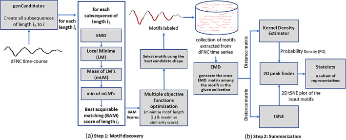
Our proposed methodology for time series motifs discovery and summarization. (a) Step 1: Motif extraction using EMD as a similarity metric. The subroutine takes out the most repetitive pattern (possibly with multiple occurrences) of a given time course, (b) Step 2: Summarization of motifs using their probability density computed by a kernel density estimator (KDE). It takes a bag of varying length motifs and generates a concise smaller collection of the most frequent shapes/patterns representing the functional system (SZ/HC). We defined these prototypes as the statelets. The EMD distance matrix is used for both performing the tSNE and computing probability density (PD) of the motifs. The relevant processing blocks and their intuitions in Step 2 are described elaborately in Section 5.2
5.1.1. EMD layer
For a given candidate of length , the algorithm searches through the timepoints by taking all other candidates of that length and computing the EMD between them. We can consider the selected candidate as a kernel here, and the idea is to apply that kernel on the input signal to compute distances.
5.1.2. Pooling local minima
The module pools a subset of top matches (minimum distance) instead of just one across the signal. Since motifs are repeating signatures, intuitively, we scrutinize the top matches only. It decomposes the input TC into several subsections and pools the minimum from each subsection.
5.1.3. Mean of LM's and global minimum
This layer computes the mean of those local minima, representing the overall performance by that specific candidate. After finishing computation for all the candidates of , the method selects the global minimum, which corresponds to the best acquirable matching (BAM) score.
5.1.4. The best length selection
To extract most recurring transient patterns, a recommender unit optimizes two objectives using the BAM scores considering all different lengths (i) minimizing the motif's length and (ii) maximizing the similarity score. The recommender unit returns the best length for decomposing a time series.
5.1.5. Motif extraction
We have already collected information from the length selection process, that is, distance, occurrences required for motifs extraction. So, using the leading candidate as the benchmark, the subroutine collects similar nonoverlapping occurrences of local motifs across the TC and stores these motifs for creating global dominants across the subjects for a given pair.
This analysis compares the dFNC time‐series datasets across the two groups, HC and SZ. After discovering the motifs from all the dFNC time series, we have a large population of variable length patterns. Next, a group‐wise summarization is performed on these motifs.
5.2. Step 2: Summarization
The decomposition technique (motif discovery) transforms the FC into a diverse connectivity signatures manifold. Each pair of components (connection) discovers a group of shapes from all the subjects. Summarization aims to fetch the representatives of the motif's collection. The intuition is to find highly persistent patterns from all the distinctive subgroups of the population to ensure that statelets approximately capture all the diversities in the given stack of motifs. The persistence is measured from the shape's PD across the given trajectory, and the subgrouping is unveiled through the t‐distributed stochastic neighbor embedding (tSNE). Our summarization scheme weighs the tSNE points using the corresponding PD. Then, an off‐the‐shelf peak technique locates the expected prototypes with standard smoothing and proximity parameters. To run the subprocesses, the probabilistic summarization runs a module called “FindDominants”: a suite of Matlab and Python scripts consisting of four steps (a, b, c, and d) mentioned in Figure 1b to identify pairwise dominant motifs. We replicate the same analysis for both subject groups SZ and HC.
5.2.1. EMD matrix
We need the distance from each motif to all others to measure the density and to subgroup them using tSNE. Here, we use EMD again for computing the distance matrix. First, we normalize the TCs to make our distance invariant to scale and offset. Then, calculate cross EMD across the motifs, which creates a square matrix of n × n dimension where n is the number of shapes in the given collection.
5.2.2. Kernel density estimator
Our method applies KDE to calculate the PD of data instances (motifs) in the population. We incorporate a Gaussian kernel with optimal bandwidth (Sheather & Jones, 1991; Silverman, 1986) in KDE. In this setting, kernel density at a point x is given by Equation 7,
| (7) |
For ‘D’ dimensions, the formulation becomes,
| (8) |
where n is the number of samples, is the kernel with a smoothing parameter, h is called the bandwidth. The kernel is a non‐negative function and h > 0. The common practice uses the Gaussian kernel for a smoother density model, simplifying the following kernel density model.
| (9) |
here is the SD of the Gaussian components. Another crucial part of the process is to select an appropriate bandwidth (h) for the density, and several strategies for selecting (I. A. Ahmad & Amezziane, 2007; Turlach, 1993). Our approach incorporates the rule‐of‐thumb bandwidth estimator for Gaussian (Scott, 2012). The optimal choice for is following,
| (10) |
here is the SD of the samples, and is the number of total samples. The term in the equation corresponds to the distance between the sample and . So, we assign EMD distances between the shapes computed in Section 5.2.1 to assign the value of the term in the equation. Using Equation (9), KDE generates PD for all motifs in the collection.
5.2.3. tSNE using EMD
tSNE is a powerful and flexible visualization tool for high‐dimensional data by giving each datapoint a location in a two‐ or three‐dimensional map (Gisbrecht, Schulz, & Hammer, 2015; Maaten & Hinton, 2008). Decentralized stochastic neighbor embedding (dSNE) separates the data subgroups using their distance metrics (Saha et al., 2017, 2019b). In our case, tSNE considers each motif as a data point and uses the EMD matrix (computed in Section 5.2.1) to select the neighbors for the embeddings. Next, the method weighs all the points using their corresponding PD. Figure 2 presents an example of how tSNE reveals intrinsic subgroups of data collection. The color indicates the PD. The brighter, the higher. The visualizations in the subsequent steps are generated using this same plot.
FIGURE 2.

An example of tSNE using EMD distance on a collection of real motifs. Data points represent the motifs weighted by their probability density computed using KDE. X and Y axis stand for the horizontal and vertical coordinates of each point, respectively
5.2.4. Two‐dimensional mapping
Although the above tSNE map unveils the subgroups, we still need to mechanistically locate the summary prototypes. To employ the peak finder, we need to map the tSNE plot (Figure 2) to a standard discrete two‐dimensional (2D) coordinate system, for example, a 2D grid. This subroutine assigns all tSNE points to a two‐dimensional discrete system and accumulates the PD of all closely neighboring shapes onto a single cell. The strive is to make dominant points more distinguishable by increasing the frequency in the corresponding vicinity. This approach discretizes the range of coordinates into a set of integer intervals. As a result, multiple points from the tSNE plot are stacked together into a single cell, as shown in Figure 3 to summarize the PD of a close neighborhood.
FIGURE 3.
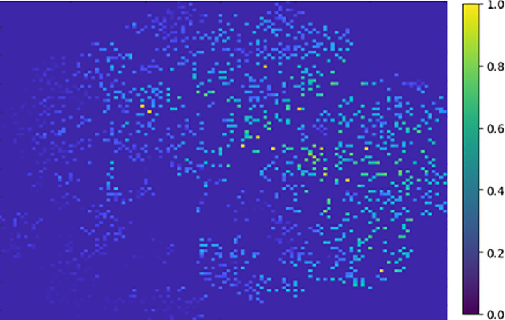
Mapping tSNE points to a 2D matrix for accumulating PD's of close neighbors. Therefore, we observe the higher density data with a brighter color in the figure
5.2.5. Gaussian blur and peak finding
Defocusing noise helps identify significant features/data points representing the subgroup. We apply a Gaussian blur to the tSNE image to facilitate the estimation of the peaks. Figure 4 displays how the blurring effect changes the focus toward relevant loci of the image. Then, we use a two‐dimensional peak finder to compute the high‐density data points. The peak finder extracts a characteristic shape from each subgroup with a higher PD. The spikes in Figure 5 indicate the representative motifs (statelets) from the whole population. It visualizes one spike per high‐density subspace. It visualizes how the summarization scheme covers the whole state‐shape trajectory and approximates the synopsis. For more clarity, the method restricts the peak finding subroutine by calibrating the smoothing parameter to avoid creating a pile of similar patterns. The objective is to find a diversified set of shapes that reasonably approximates the overall dynamics.
FIGURE 4.
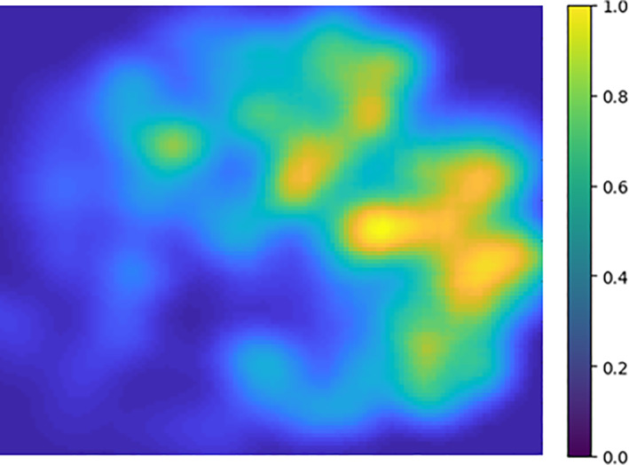
After applying a Gaussian blur on the 2D image to defocus less dense data points
FIGURE 5.
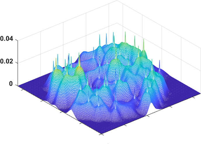
A three‐dimensional view of the tSNE plot after marking the peaks extracted by a 2D peak finder. The peak finder selects at least one peak from each high‐density region. Later, we use peak's tSNE coordinates to determine the real motifs it represents
6. EXPERIMENTAL RESULTS
We divide the dataset into 163 HC subjects and 151 SZ patients (SZ) groups. Each subject has 47 C 2 = 1,081 pairs of components or 1,081 connections: 1081 dFNC TCs. For each connection, we take TCs from all the subjects within that group (HC/SZ). Our method evaluates a subset of statelets from both groups of subjects (SZ/HC). The PD of these high dimensional state shapes denotes the consistency of these statelets across connections among multiple brain regions. In Figure 6, we show the most frequent statelets from both groups. We used the Jonker‐Volgenant algorithm (Cao, 2013) for a linear assignment problem that optimizes the mapping of tSNE coordinates to a two‐dimensional grid preserving the matching shapes in the same neighborhood constraint. In Figure 7, we compute the statelet's PD that denotes the consistency of these statelets across connections among multiple brain regions. Each bar indicates how frequently a connection's statelet has appeared in the group dynamics. The frequencies are also sorted based on their relative rank computed on their frequency in both patient and control groups. This serves to analyze the connection's readiness in the functional dynamics. We can see that the pair (connections) rank is very different in each group, suggesting a diverse influence of a connection driving the dynamics of patients versus controls. The observation indicates two distinct subsets of connection drive the group dynamics and evident a high‐level group difference in terms of neural components participating in the information processing. Further analysis is required to shed more light on these differences. Another observation is frequency of the statelets in HC connections is higher than in the SZ. To test the statistical significance of this difference between the two distributions, we compute a Kendall tau correlation coefficient, which is traditionally used to measure the ordinal association between two entities (Kendall, 1938; Puka, 2011). The hypothesis test evaluates = 0.045 with a p‐value = 0.025 indicating a statistically significant difference.
FIGURE 6.
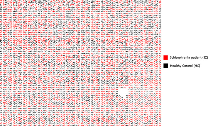
A subset of dominant motifs from SZ and HC dynamics. The motifs are detrended and visualized using tSNE followed by the Jonker‐Volgenant algorithm for the linear assignment problems. A similar type of shape is embedded into the same neighborhood. We can see a few potential subgroups of motifs. The blank space in the figure was generated because we used a larger 2D grid than the number of motifs to display. So, the algorithm optimizes the location for each motif from the 2D coordinate system to assign the matching patterns in the nearby vicinity. The X axis is time, and the Y axis represents the dynamic functional connectivity strength
FIGURE 7.
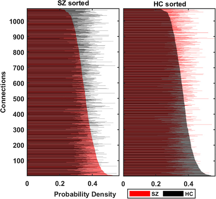
Each connection's probability density (PD) demonstrates how frequently the statelets extracted from a connection appear in the group dynamic. Each connection has two density values: one per subject group. Blue demonstrates PD in controls (HC) and red in the patients (SZ). We sort the connections low to high according to their PD in the SZ group (left subplot), and HC sorts the right subplot. Y axis represents the order of the links after sorting, and X axis depicts their corresponding PD. We observe that the rank of connections differs in both subject's groups in terms of their PD; the PD difference is statistically significant and visually evident in the plot
6.1. Dynamic features analysis
We focus more on the dynamic features of the neural system, which have been primarily unexplored in previous studies of dFNC. The dynamic properties of these representative shapes show significant group differences between HC and SZ phenotypes.
6.1.1. Recurrence
To quantify the recurrence of statelets, we use passage coding by convolving the group‐wise most frequent statelet with each connectivity time series. Passage coding annotates a time series with the corresponding convolution score and visually perceivable the repetitions. Figure 8 presents the occurrences of the group statelets in individual dynamics (randomly selected three subjects from each group). We investigated the recurrence of statelets for all the subjects and got consistent results, as shown in Figure 8. Statelets are designed to be the most generalized envelopes of brain connectivity time series; thus, higher recurrence endorses better convergence to the standard form of connectivity. The agreement toward regular co‐fluctuations by the connection aids synchronization in the brain circuitry. In the SZ dynamic, the repetitions of statelets are significantly lower than HC. That leads to a weaker association between the brain components in SZ dynamics to perform smoother cognition. Also, fewer connections are present in the SZ dynamics than HC, which indicates the absence of necessary communication among the subunits of the brain to process brain signals. Overall, the recurrence helps understand the pattern of communication (e.g., message passing) between the modules of the brain. Apparently, a more connected brain graph with the edges characterized by a recurrent communication scheme is required to produce the necessary cognitive response. This recurrence analysis indicates the absence of the necessary repetition of communications between the submodules of the brain in the SZ dynamic. This provides a ground for further study to explore the reasoning behind these abrupt connectivity patterns. Also, more analyses are required to identify why these disruptions are being triggered.
FIGURE 8.
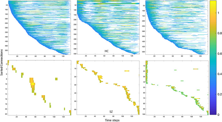
Each graph represents the occurrences of the most recurring statelets over each subject's time course. These are three randomly selected subjects from the HC (top) and SZ (bottom) groups. We convolve the group statelets with the subject dynamics (all the dFNC time courses, 1,081) to investigate the recurrence of the statelets over time. Then, we sorted the pairs based on the dominant shape's first occurrence in their time series. Consequently, the early the statelets appear in a pair's time course, the higher the pair/connection in that subject's dynamics—we threshold these convolutions matching scores at 0.8 for both groups to track down the strong appearances only. The color intensity corresponds to how strongly/weakly the shape appears in that part of the course. The color bar is identical for all the reference subjects in the figure
6.1.2. Modularity
The line graphs in Figure 11 illustrate the ensemble behavior of the connections in both dynamics (SZ/HC). The value represents the number of connections with similar prototypes at each time point. Throughout the scan session, comparatively more HC connections are activated in identical time steps than patients. This characterizes the higher modularity in the HC functional network/graph (the connections between the functional components of the brain). Modularity is imperative because it quantifies the strength of the network's division into modules. Each module consists of a subset of nodes, independent brain components in our case. These modules help data transmission by performing specific tasks independently. Results show individuals with higher baseline modularity exhibit more significant improvement with cognitive training, suggesting that a more modular baseline network state may contribute to greater adaptation in response to cognitive training (Arnemann et al., 2015). Also, cognitive ability is influenced by the relative extent of integration and segregation of functional networks (i.e., modules) distributed across distant brain regions (Chen, Abrams, & D'Esposito, 2006; Stevens et al., 2012). Subsequently, the difference in modularity is informative about the cognitive symptoms of SZ. In addition, the graph shows SZ connections become modularized at the end of the time series, whereas the HC ensembles are reduced by their size (Figure 9). This ensemble activation also demonstrates a distinct synchronization pattern between SZ and HC brains and suggests an interchanging control by various neural components.
FIGURE 9.
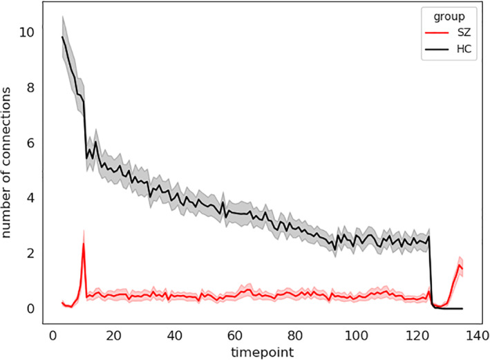
Based on probability density ranking (in Figure 7), we computed a collective appearance of the connections across all the subjects. The X axis shows the time steps, and the Y axis corresponds to the number of pairs connections that show the first statelet at that step, which indicates the activation of the pair
6.1.3. Consistency graphs
To measure the statelets' temporal consistency in the connectivity time series, we introduced a metric called TD. The primary motivation behind introducing TD is to approximate the temporal consistency of the statelets. Also, measuring how frequently these generalized dominant patterns appear in the timeline. The metric indicates how temporally localized or widespread the statelets are. TD is defined as follows.
TD: a temporal consistency measure—The TD approximates how consistently a pair's connectivity exhibits the dominant motif in the TC. The metric captures the temporal information of the summary shapes and integrates it across a group dynamic. The following equation describes TD.
| (11) |
Here, |S| = The total number of subjects in the group SZ/HC and T i the index at which the pair has appeared for the first time in a subject (T i = 1 to 136). If the pair is not present in a subject's dynamic, then T i = thus, TD for that pair in a subject is zero. We calculate the TD for each connection in a subject's dynamic and lately compute the average across the subjects within a group (SZ/HC). We used the meantime decay computed on the group dynamic for the group representation. We consider the appearance of a connection in a subject's dynamic based on the first occurrence of group statelet on that time series. The occurrence is calculated based on a thresholded convolution score. We also sorted the connection based on their first initialization in the subject's dFNC. The intuition was to investigate which connections are responsible for triggering the convergence toward statelets and how it propagates the dominance across the TC. The expected time point at which the connection is initiated in the dynamic is inverted. So, if the TD is very localized, then the mean is very close to that time point and has a higher value. In essence, it quantifies the temporal uniformity of the statelets in a subject's dynamic. Since statelets are the most repeated, stable, and representative subsequences of the time series, this attribute can potentially explain the connection's affinity toward a more generic connectivity state contributing to the dynamics. Also, TD estimates how quickly/lately the connectivity rectifies their initial disparity and converges to routine cognition. It characterizes a connection as consistently late (low TD value), consistently early (high TD value), pseudo‐random positioning (medium TD value, e.g., 0.10 to 0.15), consistent but sparse in the group dynamics (0.5–0.9), etc.
Figure 10 demonstrates the average TD graphs computed on both dynamics. Here, the vertices are independent brain networks, and the edge represents the connection between two functional networks. The weight of the edge stands for the TD; the darker, the higher. As we can see, HC functional networks are firmly connected, and most of the connections (out of 1,081) pass the TD benchmark. On the other hand, only a small subset of SZ connections converges to their group statelets. This provides evidence that the consistency of SZ network connections is considerably lower than HC. The functional connections between different brain components show more substantial temporal consistency in HC. SZ statelets are more dispersed along the timeline, consequently lacking the expected connectivity signature in the active channels. It might impact overall information processing due to a deficiency in temporally sensitive message passing in the functional network. To further probe the interconnections, we computed the transitivity of each subject's TD graph. Figure 11 shows the histograms of transitivity of subject‐wise TD graphs in both groups. Transitivity symbolizes the global probability of the network (connectivity graph) to have adjacent nodes interconnected, revealing the existence of tightly connected communities, e.g., clusters and subgroups. Most of the SZ graphs have zero or very low transitivity compared to HCs. We compute a two‐sample t test on the transitivity scores from both groups, and the p‐value, p = 9.23e‐88, indicates the difference is highly statistically significant. Higher transitivity suggests that modules in the network consistent with prior work showing increased modularity are linked to improved cognitive performance (Arnemann et al., 2015). The analysis indicates that HC networks intercommunicate more consistently and keep the channels up than SZ. This result is consistent with previous work (Allen et al., 2014; Karlsgodt, Sun, & Cannon, 2010; Rashid et al., 2014), which suggested that patients exhibit more erratic and less efficient communication among brain regions than controls. Figure 12 shows the average TD of each connection in both SZ and HC groups. The rightmost map shows HC‐SZ group differences. All the pairs in HC show a more substantial TD than SZ, especially in visual, SM, and default mode (DM) regions. Notably, HC subjects show higher TD than patients with SZ, and the apparent group differences present almost all over the brain. That also makes the data more useful for classification. Intuitively, we feed subject‐wise TD data to multiple classifiers and get good accuracy in every case. To avoid bias, the statelets are extracted from the whole dataset without using group (SZ/HC) information (unsupervised). Thus, the classification accuracies are reasonably comparable. For clarity, we can consider it a dimensionality reduction method like principal component analysis (PCA) (Wold, Esbensen, & Geladi, 1987) for better features selection. We compare the performance between running the models directly on the dFNC matrix and methods like PCA (Wold et al., 1987) for better features selection. We compare the performance between running the models directly on the dFNC matrix and the subject‐wise TD. We use multiple classifiers to test TD and observe significant accuracy improvement for more robustness. Figure 13 shows how the models perform in both cases. We can see a simple SVM or logistic regression model using TD outperforms all other methods, including LSTM with attention.
FIGURE 10.
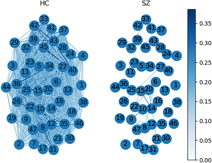
Time decay graphs from both groups. The nodes are functional networks, edges correspond to the connection between them (maximum 1,081 possible), and the weight represents the mean time decay (TD) of a connection within a group dynamic. We compute color scaling from the 95 percentiles of the total values. After thresholding at average group mean (SZ group mean + HC group mean)/2, 1,061 edges survive in the HC group and only 16 edges in the SZ group
FIGURE 11.
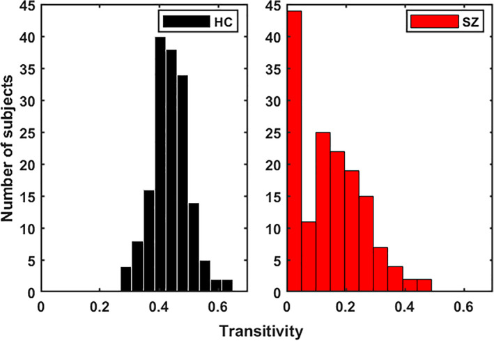
Histogram of transitivity from subject‐wise time decay graphs. It refers to the extent to which the relation between two nodes in a network connected by an edge is transitive. A significant portion of SZ subjects shows 0 transitivity, which means the connections are less consistent across different subjects. We show the differences are statistically significant using a two‐sample t‐test on both distributions. Transitivity is also related to the clustering coefficient
FIGURE 12.
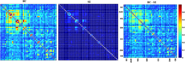
Pairwise mean time decays in healthy control (HC) and schizophrenia (SZ) groups. We run a two sample t test on the pairwise time decay values to check the statistical significance of their HC‐SZ group differences. The rightmost subfigure represents the FDR corrected t values
FIGURE 13.
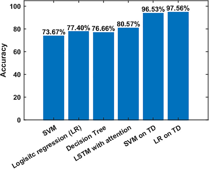
Classification accuracy for different methods. First, three methods were applied to the dFNC matrix and LSTM with the attention model applied to the dFNC time course. The last two methods use time decay (TD) for classification. We run the models on time decay information of all the subjects for 100 repeated iterations, and the accuracies are mean across the iterations. We train the model on 200 random samples in each iteration and cross‐validate them using the remaining 114 subjects
dFNC states from statelets—In this cross‐group analysis, we focus on obtaining statelets across the dataset without separating SZ and HC subjects into two different bins. The major objectives can be articulated (i) extracting cross‐group patterns, (ii) subgrouping the subjects based on statelets, (iii) experimenting with the statelet's connectivity strength and evaluating domain‐wise group differences. It is identical to the group‐wise analysis motif extraction followed by probabilistic summarization. The key difference is we send all the time series (from both subject's group HC/SZ) together through our statelet framework. Then, using approximated statelets as the representative, we partition the collection of shapes into several subgroups (connectivity states). After that, we use the EMD of extracted motifs to determine their association toward a specific subgroup/state—assign motifs to the nearest (lowest EMD) state. Statelets characterize the intrinsic cluster in the motifs extracted from dFNC TCs. The centroids of these clusters are referred to as brain states. We represent these connectivity patterns extracted from the dFNC TC as dFNC states. The centroids of these states represent patterns of FNC (temporal coherence) that individuals move between throughout the course of the experiment. We evaluate the HC‐SZ group differences in connectivity strength across the subjects within a state. For measuring the statistical significance of these differences, we use a two‐sample t test. The t‐values provide significant group differences in connectivity strength throughout the distinct regions of the brain (Figure 14). HC subjects in state 1 show stronger connections than SZ, and differences are statistically significant in SM, CC, and DM regions. In states 2 and 3, the differences are mostly HC < SZ; in state 3, group differences are statistically significant across the brain but similar strength in the connections between SB and other domains. State 4 shows mostly weaker differences except for a few auditory (AUD) and SB components, demonstrating SZ subjects are more strongly connected than HC in those regions. Two connections between AUD and DM show a statistically significant difference in state 5, and state 6 exhibits HC > SZ in the CC region. Above all, states 7, 8, and 9 show significant connectivity differences in CC and DM regions. Specifically, state 7 depicts HC > SZ and 8 and 9 shows HC < SZ group distinction. In an earlier study (Rashid et al., 2014), strong group differences are mostly in visual and AUD, but we got differences in SM, CC, and CB. We got both HC < SZ and SZ < HC in SM, CC, and DM. We observe the most significant pattern of group differences here in CC, DM, and CB regions. This triangle shows the variation in connectivity between patients and controls across multiple states with an alternating directionality, which indicates a potential biomarker for specific subtypes of SZ.
FIGURE 14.
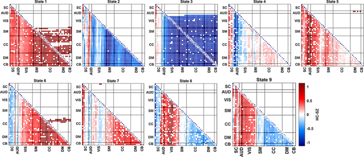
HC—SZ group differences in terms of max connectivity strength. State‐wise group differences in functional connectivity (FC). We have both SZ and HC subjects' groups at each state. For each pair of components, we have a subset of statelets from HC subjects and a subset from SZ subjects. Then, we compute the maximum connectivity strength of those statelets from both subgroups. A two‐sample t test using a null hypothesis of “No group difference” compares patients' max connectivity versus controls. A higher t value indicates the rejection of the null hypothesis irrespective of their sign. However, the sign of t values represents the directionality of the group difference. The pair matrix (47 × 47) is labeled into seven different domains subcortical (SB), auditory (AUD), visual (VIS), sensorimotor (SM), cognitive control (CC), defaultmode (DM), cerebellar (CB), respectively. White cells in the matrix indicate either the absence of that pair or nonsignificant group differences for this pair within a state. The upper triangle represents the FDR corrected differences
7. CONCLUSION
We proposed a novel method for analyzing dynamic FC via extracting high‐frequency texture from the connectivity space. To our best knowledge, it is the first pattern mining application on dFNC data. The proposed framework addresses issues in current dFNC analysis methods by modeling the dynamics through brief connectivity shapes. The analysis of those motifs enables measuring the characteristics of brain circuitry and network organization. The major contributions of our study are two‐folded, an unsupervised method for motifs discovery using EMD as a distance metric and a probabilistic summarization of these patterns. Because of the complexity of the data, it was necessary to summarize the information into a predictable and concise subspace. To do this, we included a representative snippet of the human brain connectivity graph, using the set of components as reduced space to show how it behaves over time. The experiments facilitate the observation of distinguishing connectivity signatures and the interplay among the hubs to process information. Statelets provide this summary that includes abstraction, analytics, and current trends at a glance. The statelet approach seeks an improved understanding of connectivity states and the mechanism through which their dynamics vary across individuals. Results demonstrate how these state movies help to investigate the dynamic properties of an inherently dynamic system (i.e., brain). Our approach is more robust to noise while observing short‐length dynamic features of the functional dynamics of the brain. These connectivity shapes from SZ and HC dynamics help create a global contrast between healthy and diseased brains and illustrate crucial group differences in several dynamic properties such as recurrence, modularity, and synchronizability. Our method has some limitations and potential future improvements too. That includes high time complexity and parameters tuning. We are working on a dynamic programming implementation of motif extractions to reduce the time complexity to a polynomial order—also, a framework for automatic fine‐tuning of the model's free parameters. However, statelets provide shape‐based analytics and outlines of the dynamics for the first time. It enriches our understanding of how networks communicate in spontaneous brain activity and the pattern of binding/impairment between them to maximize information transfer and minimize connection costs. We believe this would fill in a gap in the field that will help us understand the dynamics better, possibly providing an improved way to study neuropsychiatric disorders more effectively.
CONFLICT OF INTERESTS
There is no conflict of interest.
AUTHOR CONTRIBUTIONS
Vince D. Calhoun and Md Abdur Rahaman proposed the idea of statelets. Md Abdur Rahaman and Sergey M. Plis developed the methodology. Md Abdur Rahaman ran the experiments and drafted the manuscript. Sergey M. Plis helped to design a few experiments and edited the manuscript. Vince D. Calhoun supervised the whole project, thoroughly edited the article, and gave valuable feedback on the results. Eswar Damaraju provided the data and performed the preprocessing. Eswar Damaraju and Debbrata K. Saha helped run the experiments and significantly contributed to the manuscript. All authors have approved the final version of the submission.
ACKNOWLEDGMENTS
The study was funded in part by National Institute of Health (NIH) grant numbers R01MH094524, R01MH118695, R01EB020407.
Rahaman, M. A. , Damaraju, E. , Saha, D. K. , Plis, S. M. , & Calhoun, V. D. (2022). Statelets: Capturing recurrent transient variations in dynamic functional network connectivity. Human Brain Mapping, 43(8), 2503–2518. 10.1002/hbm.25799
Funding information National Institute of Health, USA (NIH), Grant/Award Numbers: R01EB020407, R01MH094524, R01MH118695
DATA AVAILABILITY STATEMENT
The dataset used in this study was collected ten years ago and included no data‐sharing agreement. Based on the IRB data privacy agreement, we are not allowed to share any subject‐specific data. However, the resting‐state fMRI data can be requested from the following link (cf. https://www.ncbi.nlm.nih.gov/pmc/articles/PMC4651841/). The pre‐processing pipelines are public, as referred to in the manuscript. All the pre‐processing tools are available online at http://trendscenter.org/software and the statelet approach will also be released within the dynamic functional network connectivity toolbox within the GIFT software package.
REFERENCES
- Agcaoglu, O. , Wilson, T. W. , Wang, Y. P. , Stephen, J. M. , & Calhoun, V. D. (2020). Dynamic resting‐state connectivity differences in eyes open versus eyes closed conditions. Brain Connectivity, 10(9), 504–519. [DOI] [PMC free article] [PubMed] [Google Scholar]
- Ahmad, I. A. , & Amezziane, M. (2007). A general and fast convergent bandwidth selection method of kernel estimator. Journal of Nonparametric Statistics, 19(4–5), 165–187. [Google Scholar]
- Ahmad, S. , Taskaya‐Temizel, T. , & Ahmad, K. (2004). Summarizing time series: Learning patterns in ‘volatile’ series. In International conference on intelligent data engineering and automated learning. Exeter, England: Springer. [Google Scholar]
- Aine, C. J. , Bockholt, H. J. , Bustillo, J. R. , Cañive, J. M. , Caprihan, A. , Gasparovic, C. , … Calhoun, V. D. (2017). Multi‐modal neuroimaging in schizophrenia: Description and dissemination. Neuroinformatics, 15(4), 343–364. [DOI] [PMC free article] [PubMed] [Google Scholar]
- Alavash, M. , Tune, S. , & Obleser, J. (2019). Modular reconfiguration of an auditory control brain network supports adaptive listening behavior. Proceedings of the National Academy of Sciences, 116(2), 660–669. [DOI] [PMC free article] [PubMed] [Google Scholar]
- Allen, E. A. , Erhardt, E. B. , Damaraju, E. , Gruner, W. , Segall, J. M. , Silva, R. F. , … Calhoun, V. D. (2011). A baseline for the multivariate comparison of resting‐state networks. Frontiers in Systems Neuroscience, 5, 2. [DOI] [PMC free article] [PubMed] [Google Scholar]
- Allen, E. A. , Damaraju, E. , Plis, S. M. , Erhardt, E. B. , Eichele, T. , & Calhoun, V. D. (2014). Tracking whole‐brain connectivity dynamics in the resting state. Cerebral Cortex, 24(3), 663–676. [DOI] [PMC free article] [PubMed] [Google Scholar]
- Alnæs, D. , Kaufmann, T. , van der Meer, D. , Córdova‐Palomera, A. , Rokicki, J. , Moberget, T. , … Karolinska Schizophrenia Project Consortium . (2019). Brain heterogeneity in schizophrenia and its association with polygenic risk. JAMA Psychiatry, 76(7), 739–748. [DOI] [PMC free article] [PubMed] [Google Scholar]
- Andoni, A. , Indyk, P. , & Krauthgamer, R. (2008). Earth mover distance over high‐dimensional spaces. in Proceedings of the nineteenth annual ACM‐SIAM symposium on Discrete algorithms. Philadelphia, PA: Society for Industrial and Applied Mathematics. [Google Scholar]
- Arnemann, K. L. , Chen, A. J. , Novakovic‐Agopian, T. , Gratton, C. , Nomura, E. M. , & D'Esposito, M. (2015). Functional brain network modularity predicts response to cognitive training after brain injury. Neurology, 84(15), 1568–1574. [DOI] [PMC free article] [PubMed] [Google Scholar]
- Bassett, D. S. , & Sporns, O. (2017). Network neuroscience. Nature Neuroscience, 20(3), 353–364. [DOI] [PMC free article] [PubMed] [Google Scholar]
- Betzel, R. F. , & Bassett, D. S. (2017). Multi‐scale brain networks. NeuroImage, 160, 73–83. [DOI] [PMC free article] [PubMed] [Google Scholar]
- Buckner, R. L. , Krienen, F. M. , & Yeo, B. T. (2013). Opportunities and limitations of intrinsic functional connectivity MRI. Nature Neuroscience, 16(7), 832–837. [DOI] [PubMed] [Google Scholar]
- Bullmore, E. , & Sporns, O. (2009). Complex brain networks: Graph theoretical analysis of structural and functional systems. Nature Reviews Neuroscience, 10(3), 186–198. [DOI] [PubMed] [Google Scholar]
- Calhoun, V. D. , Liu, J. , & Adalı, T. (2009). A review of group ICA for fMRI data and ICA for joint inference of imaging, genetic, and ERP data. NeuroImage, 45(1), S163–S172. [DOI] [PMC free article] [PubMed] [Google Scholar]
- Calhoun, V. D. , Adali, T. , Pearlson, G. D. , & Pekar, J. J. (2001). A method for making group inferences from functional MRI data using independent component analysis. Human Brain Mapping, 14(3), 140–151. [DOI] [PMC free article] [PubMed] [Google Scholar]
- Cao, Y. , LAPJV—Jonker‐Volgenant algorithm for linear assignment problem, v3. 0. Mathworks File Exchange. Retrieved from http://www.mathworks.com/matlabcentral/fileexchange, 2013. 26836.
- Champion, T. , De Pascale, L. , & Juutinen, P. (2008). The ∞‐Wasserstein distance: Local solutions and existence of optimal transport maps. SIAM Journal on Mathematical Analysis, 40(1), 1–20. [Google Scholar]
- Chen, A. J.‐W. , Abrams, G. M. , & D'Esposito, M. (2006). Functional reintegration of prefrontal neural networks for enhancing recovery after brain injury. The Journal of Head Trauma Rehabilitation, 21(2), 107–118. [DOI] [PubMed] [Google Scholar]
- Damaraju, E. , Allen, E. A. , Belger, A. , Ford, J. M. , McEwen, S. , Mathalon, D. H. , … Calhoun, V. D. (2014). Dynamic functional connectivity analysis reveals transient states of dysconnectivity in schizophrenia. NeuroImage: Clinical, 5, 298–308. [DOI] [PMC free article] [PubMed] [Google Scholar]
- Du, Y. , Fu, Z. , Sui, J. , Gao, S. , Xing, Y. , Lin, D. , … Calhoun, V. D. (2019). NeuroMark: An adaptive independent component analysis framework for estimating reproducible and comparable fMRI biomarkers among brain disorders. MedRxiv, 19008631. [Google Scholar]
- Erhardt, E. B. , Rachakonda, S. , Bedrick, E. J. , Allen, E. A. , Adali, T. , & Calhoun, V. D. (2011). Comparison of multi‐subject ICA methods for analysis of fMRI data. Human Brain Mapping, 32(12), 2075–2095. [DOI] [PMC free article] [PubMed] [Google Scholar]
- Esfahlani, F. Z. , Jo, Y. , Faskowitz, J. , Byrge, L. , Kennedy, D. P. , Sporns, O. , & Betzel, R. F. (2020). High‐amplitude cofluctuations in cortical activity drive functional connectivity. Proceedings of the National Academy of Sciences, 117(45), 28393–28401. [DOI] [PMC free article] [PubMed] [Google Scholar]
- Espinoza, F. A. , Liu, J. , Ciarochi, J. , Turner, J. A. , Vergara, V. M. , Caprihan, A. , … Calhoun, V. D. (2019). Dynamic functional network connectivity in Huntington's disease and its associations with motor and cognitive measures. Human Brain Mapping, 40(6), 1955–1968. [DOI] [PMC free article] [PubMed] [Google Scholar]
- Faskowitz, J. , Esfahlani, F. Z. , Jo, Y. , Sporns, O. , & Betzel, R. F. (2020). Edge‐centric functional network representations of human cerebral cortex reveal overlapping system‐level architecture. Nature Neuroscience, 23(12), 1644–1654. [DOI] [PubMed] [Google Scholar]
- Freire, L. , & Mangin, J.‐F. (2001). Motion correction algorithms may create spurious brain activations in the absence of subject motion. NeuroImage, 14(3), 709–722. [DOI] [PubMed] [Google Scholar]
- Friedman, J. , Hastie, T. , & Tibshirani, R. (2008). Sparse inverse covariance estimation with the graphical lasso. Biostatistics, 9(3), 432–441. [DOI] [PMC free article] [PubMed] [Google Scholar]
- Friston, K. J. , & Frith, C. D. (1995). Schizophrenia: A disconnection syndrome. Clinical Neuroscience, 3(2), 89–97. [PubMed] [Google Scholar]
- Gisbrecht, A. , Schulz, A. , & Hammer, B. (2015). Parametric nonlinear dimensionality reduction using kernel t‐SNE. Neurocomputing, 147, 71–82. [Google Scholar]
- Grandjean, J. , Preti, M. G. , Bolton, T. A. , Buerge, M. , Seifritz, E. , Pryce, C. R. , … Rudin, M. (2017). Dynamic reorganization of intrinsic functional networks in the mouse brain. NeuroImage, 152, 497–508. [DOI] [PubMed] [Google Scholar]
- Hilger, K. , Fukushima, M. , Sporns, O. , & Fiebach, C. J. (2020). Temporal stability of functional brain modules associated with human intelligence. Human Brain Mapping, 41(2), 362–372. [DOI] [PMC free article] [PubMed] [Google Scholar]
- Hyvärinen, A. , & Oja, E. (2000). Independent component analysis: Algorithms and applications. Neural Networks, 13(4–5), 411–430. [DOI] [PubMed] [Google Scholar]
- Jafri, M. J. , Pearlson, G. D. , Stevens, M. , & Calhoun, V. D. (2008). A method for functional network connectivity among spatially independent resting‐state components in schizophrenia. NeuroImage, 39(4), 1666–1681. [DOI] [PMC free article] [PubMed] [Google Scholar]
- Kacprzyk, J. , Wilbik, A. , & Zadrożny, S. (2008). Linguistic summarization of time series using a fuzzy quantifier driven aggregation. Fuzzy Sets and Systems, 159(12), 1485–1499. [Google Scholar]
- Karlsgodt, K. H. , Sun, D. , & Cannon, T. D. (2010). Structural and functional brain abnormalities in schizophrenia. Current Directions in Psychological Science, 19(4), 226–231. [DOI] [PMC free article] [PubMed] [Google Scholar]
- Keator, D. B. , van Erp, T. G. , Turner, J. A. , Glover, G. H. , Mueller, B. A. , Liu, T. T. , … Potkin, S. G. (2016). The function biomedical informatics research network data repository. NeuroImage, 124(Pt B), 1074–1079. [DOI] [PMC free article] [PubMed] [Google Scholar]
- Kendall, M. G. (1938). A new measure of rank correlation. Biometrika, 30(1/2), 81–93. [Google Scholar]
- Levina, E. , & Bickel, P. (2001). The earth mover's distance is the mallows distance: Some insights from statistics. in Proceedings Eighth IEEE International Conference on Computer Vision. ICCV 2001. Vancouver, Canada: IEEE. [Google Scholar]
- Liang, M. , Zhou, Y. , Jiang, T. , Liu, Z. , Tian, L. , Liu, H. , & Hao, Y. (2006). Widespread functional disconnectivity in schizophrenia with resting‐state functional magnetic resonance imaging. Neuroreport, 17(2), 209–213. [DOI] [PubMed] [Google Scholar]
- Liao, X. , Cao, M. , Xia, M. , & He, Y. (2017). Individual differences and time‐varying features of modular brain architecture. NeuroImage, 152, 94–107. [DOI] [PubMed] [Google Scholar]
- Lin, J. , Keogh Eamonn, Lonardi Stefano, Patel Pranav, Finding Motifs in Time Series. Proceedings of the Second Workshop on Temporal Data Mining, 2002.
- Liu, F. , Wang, Y. , Li, M. , Wang, W. , Li, R. , Zhang, Z. , … Chen, H. (2017). Dynamic functional network connectivity in idiopathic generalized epilepsy with generalized tonic–clonic seizure. Human Brain Mapping, 38(2), 957–973. [DOI] [PMC free article] [PubMed] [Google Scholar]
- Luchins, D. J. , Weinberger, D. R. , & Wyatt, R. J. (1979). Schizophrenia: Evidence of a subgroup with reversed cerebral asymmetry. Archives of General Psychiatry, 36(12), 1309–1311. [DOI] [PubMed] [Google Scholar]
- Lynall, M.‐E. , Bassett, D. S. , Kerwin, R. , McKenna, P. J. , Kitzbichler, M. , Muller, U. , & Bullmore, E. (2010). Functional connectivity and brain networks in schizophrenia. Journal of Neuroscience, 30(28), 9477–9487. [DOI] [PMC free article] [PubMed] [Google Scholar]
- Ma, S. , Calhoun, V. D. , Phlypo, R. , & Adalı, T. (2014). Dynamic changes of spatial functional network connectivity in healthy individuals and schizophrenia patients using independent vector analysis. NeuroImage, 90, 196–206. [DOI] [PMC free article] [PubMed] [Google Scholar]
- Maaten, L.v.d. , & Hinton, G. (2008). Visualizing data using t‐SNE. Journal of Machine Learning Research, 9(11), 2579–2605. [Google Scholar]
- Miller, R. L. , Yaesoubi, M. , Turner, J. A. , Mathalon, D. , Preda, A. , Pearlson, G. , … Calhoun, V. D. (2016). Higher dimensional meta‐state analysis reveals reduced resting fMRI connectivity dynamism in schizophrenia patients. PLoS One, 11(3), e0149849. [DOI] [PMC free article] [PubMed] [Google Scholar]
- Morioka, H. , Calhoun, V. , & Hyvärinen, A. (2020). Nonlinear ICA of fMRI reveals primitive temporal structures linked to rest, task, and behavioral traits. NeuroImage, 218, 116989. [DOI] [PMC free article] [PubMed] [Google Scholar]
- Mueen, A. (2014). Time series motif discovery: Dimensions and applications. Wiley Interdisciplinary Reviews: Data Mining and Knowledge Discovery, 4(2), 152–159. [Google Scholar]
- Petersen, S. E. , & Sporns, O. (2015). Brain networks and cognitive architectures. Neuron, 88(1), 207–219. [DOI] [PMC free article] [PubMed] [Google Scholar]
- Power, J. D. , Cohen, A. L. , Nelson, S. M. , Wig, G. S. , Barnes, K. A. , Church, J. A. , … Petersen, S. E. (2011). Functional network organization of the human brain. Neuron, 72(4), 665–678. [DOI] [PMC free article] [PubMed] [Google Scholar]
- Puka, L. (2011). Kendall's Tau. In Lovric M. (Ed.), International Encyclopedia of Statistical Science (pp. 713–715). Berlin Heidelberg: Springer. [Google Scholar]
- Rahaman, M. A. , Turner, J. A. , Gupta, C. N. , Rachakonda, S. , Chen, J. , Liu, J. , … Calhoun, V. D. (2019). N‐BiC: A method for multi‐component and symptom biclustering of structural MRI data: Application to schizophrenia. IEEE Transactions on Biomedical Engineering, 67(1), 110–121. [DOI] [PMC free article] [PubMed] [Google Scholar]
- Rahaman, M. A. , Damaraju, E. , Turner, J. A. , van Erp, T. G. , Mathalon, D. , Vaidya, J. , … Calhoun, V. D. (2020). A novel method for tri‐clustering dynamic functional network connectivity (dFNC) identifies significant schizophrenia effects across multiple states in distinct subgroups of individuals. Brain Connectivity, 12(1), 61–73. [DOI] [PMC free article] [PubMed] [Google Scholar]
- Rashid, B. , Damaraju, E. , Pearlson, G. D. , & Calhoun, V. D. (2014). Dynamic connectivity states estimated from resting fMRI identify differences among schizophrenia, bipolar disorder, and healthy control subjects. Frontiers in Human Neuroscience, 8, 897. [DOI] [PMC free article] [PubMed] [Google Scholar]
- Rashid, B. , Arbabshirani, M. R. , Damaraju, E. , Cetin, M. S. , Miller, R. , Pearlson, G. D. , & Calhoun, V. D. (2016). Classification of schizophrenia and bipolar patients using static and dynamic resting‐state fMRI brain connectivity. NeuroImage, 134, 645–657. [DOI] [PMC free article] [PubMed] [Google Scholar]
- Rubner, Y. , Tomasi, C. , & Guibas, L. J. (2000). The earth mover's distance as a metric for image retrieval. International Journal of Computer Vision, 40(2), 99–121. [Google Scholar]
- Rüschendorf, L. (1985). The Wasserstein distance and approximation theorems. Probability Theory and Related Fields, 70(1), 117–129. [Google Scholar]
- Saha, D. K. , Calhoun, V. D. , Panta, S. R. , & Plis, S. M. (2017). See without looking: Joint visualization of sensitive multi‐site datasets. In IJCAI. (pp. 2672–2678). Melbourne, Australia: AAAI Press. [Google Scholar]
- Saha, D. K. , Abrol, A. , Damaraju, E. , Rashid, B. , Plis, S. M. , & Calhoun, V. D. (2019a). Classification as a criterion to select model order for dynamic functional connectivity states in rest‐fMRI data. In 2019 IEEE 16th International Symposium on Biomedical Imaging (ISBI 2019). Venice, Italy: IEEE. [Google Scholar]
- Saha, D. K. , Calhoun, V. D. , Yuhui, D. , Zening, F. , Panta, S. R. , & Plis, S. M. (2019b). dSNE: A visualization approach for use with decentralized data. BioRxiv, 826974. [Google Scholar]
- Sakoğlu, Ü. , Pearlson, G. D. , Kiehl, K. A. , Wang, Y. M. , Michael, A. M. , & Calhoun, V. D. (2010). A method for evaluating dynamic functional network connectivity and task‐modulation: Application to schizophrenia. Magnetic Resonance Materials in Physics, Biology and Medicine, 23(5), 351–366. [DOI] [PMC free article] [PubMed] [Google Scholar]
- Scarr, E. , Cowie, T. F. , Kanellakis, S. , Sundram, S. , Pantelis, C. , & Dean, B. (2009). Decreased cortical muscarinic receptors define a subgroup of subjects with schizophrenia. Molecular Psychiatry, 14(11), 1017–1023. [DOI] [PubMed] [Google Scholar]
- Scott, D. W. (2012). Multivariate density estimation and visualization. In Handbook of computational statistics (pp. 549–569). Berlin, Germany: Springer. [Google Scholar]
- Sheather, S. J. , & Jones, M. C. (1991). A reliable data‐based bandwidth selection method for kernel density estimation. Journal of the Royal Statistical Society: Series B: Methodological, 53(3), 683–690. [Google Scholar]
- Siebenhühner, F. , Weiss, S. A. , Coppola, R. , Weinberger, D. R. , & Bassett, D. S. (2013). Intra‐ and inter‐frequency brain network structure in health and schizophrenia. PLoS One, 8(8), e72351. [DOI] [PMC free article] [PubMed] [Google Scholar]
- Silverman, B. W. (1986). Density estimation for statistics and data analysis (Vol. 26). Boca Raton, FL: CRC press. [Google Scholar]
- Smith, S. M. , Miller, K. L. , Salimi‐Khorshidi, G. , Webster, M. , Beckmann, C. F. , Nichols, T. E. , … Woolrich, M. W. (2011). Network modelling methods for FMRI. NeuroImage, 54(2), 875–891. [DOI] [PubMed] [Google Scholar]
- Sporns, O. , Faskowitz, J. , Teixeira, A. S. , Cutts, S. A. , & Betzel, R. F. (2020). Dynamic expression of brain functional systems disclosed by fine‐scale analysis of edge time series. Network Neuroscience, 5, 405–433. [DOI] [PMC free article] [PubMed] [Google Scholar]
- Sripada, S. , Reiter, E. , Hunter, J. , & Yu, J. Summarizing neonatal time series data. In 10th Conference of the European Chapter of the Association for Computational Linguistics. 2003.
- Stephan, K. E. , Baldeweg, T. , & Friston, K. J. (2006). Synaptic plasticity and dysconnection in schizophrenia. Biological Psychiatry, 59(10), 929–939. [DOI] [PubMed] [Google Scholar]
- Stevens, A. A. , Tappon, S. C. , Garg, A. , & Fair, D. A. (2012). Functional brain network modularity captures inter‐and intra‐individual variation in working memory capacity. PLoS One, 7(1), e30468. [DOI] [PMC free article] [PubMed] [Google Scholar]
- Torkamani, S. , & Lohweg, V. (2017). Survey on time series motif discovery. Wiley Interdisciplinary Reviews: Data Mining and Knowledge Discovery, 7(2), e1199. [Google Scholar]
- Tsuang, M. T. , Lyons, M. J. , & Faraone, S. V. (1990). Heterogeneity of schizophrenia: Conceptual models and analytic strategies. British Journal of Psychiatry, 156(1), 17–26. [DOI] [PubMed] [Google Scholar]
- Turlach, B. A. (1993). Bandwidth selection in kernel density estimation: A review. In CORE and Institut de Statistique. Citeseer. Universite Catholique de Louvain. [Google Scholar]
- Vallender, S. S. (1974). Calculation of the Wasserstein distance between probability distributions on the line. Theory of Probability and its Applications, 18(4), 784–786. [Google Scholar]
- Varoquaux, G. , Gramfort, A. , Poline, J. B. , & Thirion, B. (2010). Brain covariance selection: Better individual functional connectivity models using population prior. Advances in Neural Information Processing Systems, 23, 2334–2342. [Google Scholar]
- Vergara, V. M. , Mayer, A. R. , Kiehl, K. A. , & Calhoun, V. D. (2018). Dynamic functional network connectivity discriminates mild traumatic brain injury through machine learning. NeuroImage: Clinical, 19, 30–37. [DOI] [PMC free article] [PubMed] [Google Scholar]
- Wold, S. , Esbensen, K. , & Geladi, P. (1987). Principal component analysis. Chemometrics and Intelligent Laboratory Systems, 2(1–3), 37–52. [Google Scholar]
- Yu, Q. , Allen, E. A. , Sui, J. , Arbabshirani, M. R. , Pearlson, G. , & Calhoun, V. D. (2012). Brain connectivity networks in schizophrenia underlying resting state functional magnetic resonance imaging. Current Topics in Medicinal Chemistry, 12(21), 2415–2425. [DOI] [PMC free article] [PubMed] [Google Scholar]
- Zhi, D. , Calhoun, V. D. , Lv, L. , Ma, X. , Ke, Q. , Fu, Z. , … Sui, J. (2018). Aberrant dynamic functional network connectivity and graph properties in major depressive disorder. Frontiers in Psychiatry, 9, 339. [DOI] [PMC free article] [PubMed] [Google Scholar]
- Zhou, Y. , Shu, N. , Liu, Y. , Song, M. , Hao, Y. , Liu, H. , … Jiang, T. (2008). Altered resting‐state functional connectivity and anatomical connectivity of hippocampus in schizophrenia. Schizophrenia Research, 100(1–3), 120–132. [DOI] [PubMed] [Google Scholar]
Associated Data
This section collects any data citations, data availability statements, or supplementary materials included in this article.
Data Availability Statement
The dataset used in this study was collected ten years ago and included no data‐sharing agreement. Based on the IRB data privacy agreement, we are not allowed to share any subject‐specific data. However, the resting‐state fMRI data can be requested from the following link (cf. https://www.ncbi.nlm.nih.gov/pmc/articles/PMC4651841/). The pre‐processing pipelines are public, as referred to in the manuscript. All the pre‐processing tools are available online at http://trendscenter.org/software and the statelet approach will also be released within the dynamic functional network connectivity toolbox within the GIFT software package.


